Improved representation of sequence bloom trees

Abstract

Motivation

Algorithmic solutions to index and search biological databases are a fundamental part of bioinformatics, providing underlying components to many end-user tools. Inexpensive next generation sequencing has filled publicly available databases such as the Sequence Read Archive beyond the capacity of traditional indexing methods. Recently, the Sequence Bloom Tree (SBT) and its derivatives were proposed as a way to efficiently index such data for queries about transcript presence.

Results

We build on the SBT framework to construct the HowDe-SBT data structure, which uses a novel partitioning of information to reduce the construction and query time as well as the size of the index. Compared to previous SBT methods, on real RNA-seq data, HowDe-SBT can construct the index in less than 36% of the time and with 39% less space and can answer small-batch queries at least five times faster. We also develop a theoretical framework in which we can analyze and bound the space and query performance of HowDe-SBT compared to other SBT methods.

Availability and implementation

HowDe-SBT is available as a free open source program on https://github.com/medvedevgroup/HowDeSBT.

Supplementary information

Supplementary data are available at Bioinformatics online.

1 Introduction

Public read databases such as the Sequence Read Archive (SRA) contain a treasure trove of biological information and have the potential to become a ubiquitous community resource by enabling broad exploratory analyses. For example, given a long nucleotide sequence, which experiments in the database contain reads matching it? More concretely, which human RNA-seq experiments from the SRA contain a transcript of interest? Unfortunately, there does not exist a way for today’s biologist to answer such a question in a reasonable amount of time. Tapping into the potential of these databases is hampered by scalability challenges and will require novel approaches from the algorithm community.

The computational problem falls into the widely-studied category of string alignment problems (Gusfield, 1997; Mäkinen et al., 2015). However, it differs in several regards. The strings to be matched are rarely present in the database in their entirety. Instead, sequencers produce many highly fragmented copies of the desired string, each subjected to potential sequencing error. Furthermore, the scale of the databases makes traditional sequence alignment methods, such as SRA-BLAST (Camacho et al., 2009), inadequate (Solomon and Kingsford, 2016).

The seminal paper of Solomon and Kingsford (2016) demonstrated that the above transcript question can be simplified to a question of approximate k-mer membership. Each experiment can be viewed as a collection of its constituent k-mers, and the biological question can be answered by finding all experiments which contain a high percentage of the k-mers in the query transcript. They demonstrated that this approach, even if only done approximately, is a good proxy for the answer to the transcript question. It also lends itself to answering a more broad range of questions, such as SNP presence, viral contamination, or gene fusion (Bradley et al., 2017). Their work has opened the door to a slew of data structures implementing various k-mer indices, roughly falling into two categories.

The first category of approaches are based on the Bloofi (Crainiceanu and Lemire, 2015) data structure. Each experiment’s k-mers are first stored in a Bloom filter (BF) (Bloom, 1970), an efficient but lossy data structure for storing sets. The experiments are then grouped into a hierarchical structure (i.e. tree) based on their similarity, where each leaf corresponds to the k-mers in an experiment. Each internal node represents the union of the k-mers in its descendants. The tree allows an efficient search for experiments matching a given k-mer profile by pruning non-promising branches. Bloofi was first adapted to the sequencing context by the Sequence Bloom Tree (SBT) data structure (Solomon and Kingsford, 2016), and further work improved the representation of the internal nodes (Solomon and Kingsford, 2017; Sun et al., 2018) and the clustering of the tree topology (Sun et al., 2018).

The SBT approaches aggregate k-mer information at the level of an experiment. The second category of approaches aggregate experiment information at the level of the k-mers. In such an approach, each query k-mer is independently looked up in an index to retrieve information about which experiments contain the k-mer (Almodaresi et al., 2017, 2018; Bradley et al., 2017; Holley et al., 2015; Holley and Melsted, 2019; Muggli et al., 2017; Mustafa et al., 2018; Pandey et al., 2018; Yu et al., 2018). In this context, experiments are referred to as colors, and such a data structure is sometimes called a colored de Bruijn graph. These approaches are complementary to the SBT and the best choice depends on the particular properties of the queries and the dataset, such as the sharedness of k-mers between experiments.

In this paper, we make two main contributions. First, we develop an alternative way to partition and organize the data in an SBT such that it becomes more compressible and faster to query. To demonstrate the performance advantages of our method, called HowDe-SBT, we compare it on real data to the previous SBT methods. We also propose and explore a culling procedure to remove non-informative nodes from the tree and create a non-binary forest (Supplementary Material).

Second, we introduce a theoretical framework which allows us to prove bounds on the performance of HowDe-SBT in comparison with Split-SBT (abbreviated as SSBT) (Solomon and Kingsford, 2017). Previous papers in the field have focused on experimental metrics for comparison, but, while these are very valuable and necessary, they can vary greatly depending on the dataset or the system used. Theoretical bounds can deepen our understanding of why algorithms perform well and can drive the development of better methods. In this paper, we derive an information theoretic bound on the space used by an SBT (Theorem 1) and quantify the number of bit lookups necessary for a query (Theorem 2).

2 Preliminaries

Let x and y be two bitvectors of the same length. A bitvector can be viewed as a set of the positions that are set to 1, and in this view, the set union (intersection, respectively) of x and y is equivalent to bitwise OR (AND, respectively). We write the bitwise AND between x and y as $x\cap y$⁠, and the bitwise OR as $x\cup y$⁠. The bitwise NOT operation on x is written as $\overline{x}$⁠. The set difference of x and y is written as $x\setminus y$ and can be defined as $x\setminus y=x\cap \overline{y}$⁠. The empty set is represented as a bitvector of zeros. The universal set, denoted by $\xi$⁠, is represented as a bitvector of ones. Given that the fraction of 1 s in x is p, the empirical entropy of x is defined as $H(p)=-(p{\hspace{0.17em}\text{log}\hspace{0.17em}}_{2}p+(1-p){\hspace{0.17em}\text{log}\hspace{0.17em}}_2(1-p))$⁠.

A BF is a bitvector of length b, together with q hash functions, $h_1,\dots ,h_q$⁠, where b and q are parameters. Each hash function maps a k-mer to an integer between 0 and $b-1$⁠. To add a k-mer x to the set, we set the position $h_i(x)$ to 1, for all i. To check if a k-mer x is in the set, we check that the position $h_i(x)$ is 1, for all i. Note that a false positive may occur, i.e. x may have never been added but all its corresponding positions were still set to 1 and it is considered to be contained in the BF. In this paper, we restrict the number of hash functions to be q = 1 (as is done in other SBT approaches).

Next, consider a rooted binary tree T. The parent of a non-root node u is denoted as parent(u), and the set of all the leaves of the subtree rooted at a node u is denoted by leaves(u). Let children(u) refer to the child nodes of a non-leaf node u. Define ancestors(u) as $\varnothing$ if node u is the root, and $\text{parent}(u)\cup \text{ancestors}(\text{parent}(u))$ otherwise. That is, ancestors(u) are all the nodes on the path from u to the root, except u itself.

Suppose that there is a BF associated with each leaf of T. Then, define $B_{\cup }(u)$ for a leaf node u as its associated BF and $B_{\cup }(u)$ for an internal node as $\underset{i\in \text{leaves}(u)}{\cup }{B}_{\cup }(i)$⁠. Note that $B_{\cup }(u)$ of an internal node u can be equivalently defined as $B_{\cup }(u)=\underset{i\in \text{children}(u)}{\cup }{B}_{\cup }(i)$⁠. Define the intersection of leaf BFs in the subtree rooted at a node u as $B_{\cap }(u)=\underset{i\in \text{leaves}(u)}{\cap }{B}_{\cup }(i)$⁠. Equivalently, at internal nodes, $B_{\cap }(u)=\underset{i\in \text{children}(u)}{\cap }{B}_{\cap }(i)$⁠.

In this paper, we solve the following problem:

Database input: A database $D=\{D_1,\dots ,D_n\}$⁠, where each D_i is a BF of size b that represents experiment i. Typically, D_i contains all the non-erroneous k-mers that appear in the reads of experiment i.

Query input: A multi-set of k-mers Q (called the query), and a threshold $0<\theta \le 1$⁠.

Query output: The set of experiments whose D_i contains at least a fraction θ of the query k-mers, i.e. $\{i:|\{x\in Q:x \text{exists} \text{in}{D}_i\}|\ge \theta ·|\hspace{0.17em}Q\left|\right\}$

Note that in this formulation, we assume that D (along with parameter b) is already given to us. How to choose b and construct D from raw reads was already described in Solomon and Kingsford (2016).

3 Representation and querying

Initially, we determine a tree topology T using the clustering algorithm of Sun et al. (2018) as a black-box. A topology is a binary tree with a bijection between its leaves and the experiment BFs in our database; a topology does not yet have bitvectors assigned to the internal nodes. We now show how to assign these bitvectors—B_det and B_how—and how they can be used to answer a query.

Conceptually, each node u represents the set of experiment BFs corresponding to leaves(u). We observe that some positions are determined in u: they have the same value in each of leaves(u). Moreover, for the positions that are determined, we know exactly how they are determined. Formally, we define

$$B_{\text{det}}(u)\triangleq B_{\cap }(u)\cup \overline{B_{\cup }(u)}\hspace{0.17em}\hspace{0.17em}\hspace{0.17em}\hspace{0.17em}\hspace{0.17em}\hspace{0.17em}\hspace{0.17em}\hspace{0.17em}\hspace{0.17em}\hspace{0.17em}\hspace{0.17em}\hspace{0.17em}\hspace{0.17em}{B}_{\text{how}}(u)\triangleq B_{\cap }(u)$$

(1)

Note that B_how is intended to only be informative for those positions that are in B_det.  Figure 1 shows an example of a tree and its B_det and B_how representation.

Fig. 1.

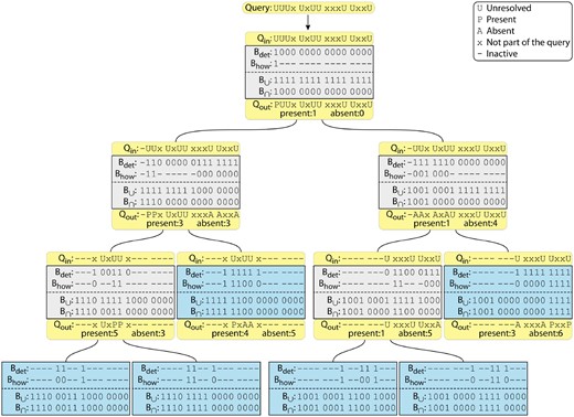
Example HowDe-SBT on $D=\{1110\hspace{0.17em}0011\hspace{0.17em}1000\hspace{0.17em}0000,$  $1110\hspace{0.17em}1111\hspace{0.17em}0000\hspace{0.17em}0000,$  $1111\hspace{0.17em}1100\hspace{0.17em}0000\hspace{0.17em}0000,$  $1001\hspace{0.17em}0001\hspace{0.17em}1100\hspace{0.17em}1000,$  $1001\hspace{0.17em}0000\hspace{0.17em}1111\hspace{0.17em}0000,$  $1001\hspace{0.17em}0000\hspace{0.17em}0000\hspace{0.17em}1111\}$⁠. Each box represents a node of the tree, with leaves shown in blue and internal nodes in gray. For conciseness, the boxes show B_det,  B_how,  $B_{\cup }$ and $B_{\cap }$⁠, but do not explicitly show $B_{\text{det}}^{\text{sqz}\hspace{0.17em}}$ and $B_{\text{how}}^{\text{sqz}\hspace{0.17em}}$⁠. The yellow boxes demonstrate the processing of an example nine k-mer query with $\theta =0.5$⁠. The initial query is shown at the top, with the bits corresponding to the query k-mers shown with a U. The query flows down the tree, i.e. it is processed in a preorder traversal. The query state presented to a node is $Q_{\text{in}}$ and the result from the node is $Q_{\text{out}}$⁠. Some bits are resolved as either present (P) or absent (A) across the subtree. Such bits are counted in the corresponding totals and removed from further processing (hyphen) in descendants. Processing along a branch halts if either total reaches the threshold needed to determine the outcome. In this example, the search along any branch can be terminated if either the present counter or the absent counter exceeds 5. In this example, Q matches the first two experiments. (Color version of this figure is available at Bioinformatics online.)

Having B_det and B_how at each node can enable the following efficient query search; it is essentially the same strategy as in Sun et al. (2018) and Solomon and Kingsford (2017), but adapted to the HowDe-SBT tree. When we receive the set of query k-mers Q, we hash each one to determine the list of BF positions corresponding to Q (recall that our BF uses only one hash function, hence each k-mer corresponds to just one position). We call this list the unresolved positions. We also maintain two counters: the number of positions that have been determined to be 1 (present), and the number of positions determined to be 0 (absent). These counters are both initially 0. We then proceed in a recursive manner, starting at the root of the tree. When comparing Q against a node u, each unresolved position that is 1 in $B_{\text{det}}(u)$ is removed from the unresolved list and the corresponding bit in $B_{\text{how}}(u)$ determines which counter, present or absent, is incremented. If the present counter is at least $\theta \left|Q\right|$⁠, we add leaves(u) to the list of matches and terminate the search of u’s subtree. If the absent counter exceeds $(1-\theta )\left|Q\right|$⁠, Q cannot match any of the descendant leaves so we terminate the search of u’s subtree. If neither of these holds, we recursively pass the two counters and the list of unresolved positions down to u’s children. When we reach a leaf, the query unresolved list will become empty because $B_{\text{det}}$ is all ones at a leaf, and the algorithm will necessarily terminate. Figure 1 shows an example of a query execution.

We observe that some bit positions will never be looked at during a search, as follows. First, if a position is determined at a node v, it will be removed from the query unresolved list (if it was even there) after node v is processed. We say that this position is inactive in v’s descendants, since a search will never query that position. Formally, a position is active in $B_{\text{det}}(u)$ if it is not determined at its parent (equivalently, at any of its ancestors). Second, the only positions that are queried in $B_{\text{how}}(u)$ are those that are active and set to one in $B_{\text{det}}(u)$⁠. We say these positions are active in $B_{\text{how}}(u)$⁠. Formally, we can define

$$B_{\text{det}}^{\text{active}\hspace{0.17em}}(u)\triangleq \{\begin{array}{cc}\overline{B_{\text{det}}(\text{parent}(u))}\hfill & \text{if} u \text{has} \mathrm{a} \text{parent}\hfill \\ \xi \hfill & \text{if} u \text{is} \text{the} \text{root}\hfill \end{array}$$

(2)

 

$$B_{\text{how}}^{\text{active}\hspace{0.17em}}(u)\triangleq B_{\text{det}}(u)\cap B_{\text{det}}^{\text{active}\hspace{0.17em}}(u)$$

(3)

Bits that are inactive are wasteful, since they take space to store but are never queried. We remove these bits, forming (usually shorter) bitvectors comprised of only the active bits. Formally, let $B_{\text{det}}^{\text{sqz}\hspace{0.17em}}(u)$ be $B_{\text{det}}(u)$ with all the inactive bits removed, and we let $B_{\text{how}}^{\text{sqz}\hspace{0.17em}}(u)$ be $B_{\text{how}}(u)$ with all the inactive bits removed. $B_{\text{det}}^{\text{sqz}\hspace{0.17em}}$ and $B_{\text{how}}^{\text{sqz}\hspace{0.17em}}$ are further compressed with the general purpose RRR compression algorithm (Raman et al., 2007), and these compressed bitvectors are what, in the end, constitute our index. We note that since the removal of inactive bits changes the indices into the bitvectors, the query algorithm has to be modified accordingly by using rank and select. Since this is done in essentially the same way as in Solomon and Kingsford (2017), we omit the details here.

4 Analysis of savings compared to previous work

In this section, we show the connection of our representation to previous approaches and analyze the theoretical improvements. The structuring of our bitvectors can be viewed as an extension of the approach in Solomon and Kingsford (2017), which is called SSBT. The SSBT representation approach subsumes the representation of Sun et al. (2018), so we focus our comparison on SSBT. Briefly, SSBT uses the same approach of having a tree where the bitvectors at a node u represent, for each bit position x, whether x is 1 in all, none, or some of the leaves(u). It also marks a bit position as inactive if it can never be reached during a query. The SSBT bitvectors are called u_sim and u_rem. The topology of the SSBT is computed differently from HowDe-SBT, and, as was shown in Sun et al. (2018), it results in a poorly clustered tree. However, since we want to focus on the improvements solely due to bitvector representation, we will assume that the SSBT is constructed using the same topology as HowDe-SBT. In this case, the relationship of SSBT to HowDe-SBT can be summarized as a one-to-one relationship between all possible bitvector states, shown in Figure 2.

Fig. 2.

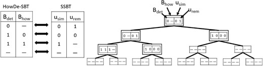
The left tables show the correspondence between the possible states of SSBT and HowDe-SBT bitvectors. A dash represents an inactive bit. The tree is an example of a bit position x and its values in both representations. The nodes of T_x have a double border. In this example, n_x = 5 and ${\ell }_x=3$ because T_x has 5 nodes and 3 leaves. Further, $s_x=1/3$ because the how bit is active in exactly three nodes (corresponding to the leaves of T_x) and set to 1 in exactly one of them

The intuition which guided our design of HowDe-SBT, relative to SSBT, was (i) minimizing the number of active positions and 1 bits (to improve space), and (ii) minimizing the number of bit lookups performed during a query (to improve speed). To try to theoretically quantify this improvement, we derive a savings rate per bit position x, in terms of (i) n_x, the number of nodes where x is active in B_det, and (ii) s_x, the percentage of nodes where x is active in B_how that have a 1.

Let T be the tree topology. We are not able to directly derive the savings rate for T after RRR compression, but we instead rely on Shannon’s information compression bound. For a bitvector a that is generated by a 0th order Markov model and that has a fraction p of 1 s, the best that a lossless compression algorithm can achieve is $\left|a\right|H(p)$ bits. While in practice this bound might be beaten because our bitvectors are not generated by a 0th order Markov chain, it is still a useful proxy for the compressibility [and in any case the RRR compression that we use does not compress beyond the 0th order bound (Raman et al., 2007)]. Let $I_x^{\text{howde}}$ (respectively, $I_x^{\text{ssbt}}$⁠) denote Shannon’s information bound for storing all the bit values at x in T using HowDe-SBT’s representation (respectively, SSBT’s representation). 

Theorem 1. Let $0\le x<b$ be a bit position. Then,

$$\begin{array}{c}{I}_x^{\text{howde}}=\frac{3n_x+1}{2}H\left(\frac{(n_x+1)(1+s_x)}{3n_x+1}\right)\\ I_x^{\text{ssbt}}=\frac{n_x(4-s_x)-s_x}{2}H\left(\frac{n_x(1+s_x)+s_x-1}{n_x(4-s_x)-s_x}\right)\end{array}$$

Proof. Let T_x be the subtree of T containing all nodes where x is active in B_det. Observe that T_x is indeed a subtree and it contains exactly the nodes where x is determined and their ancestors. The total number of nodes in T_x is n_x. Let ${\ell }_x$ be the number of leaves of T_x. Note that since every internal node of T has two children, ${\ell }_x=(n_x+1)/2$⁠, for all x. Note that the nodes at which the B_how bits are active are exactly the leaves of T_x, and s_x is the percentage of these that are 1.

Now, the nodes for which x is active in $B_{\text{det}}$ are exactly the nodes of T_x, and thus x contributes n_x active B_det bits. The only time B_how is active at x is when B_det is set to 1, which is exactly at the leaves of T_x. Hence, the total number of active bits is $n_x+{\ell }_x=(3n_x+1)/2$⁠. Next, we count the number of active bits that are set to 1. The B_det bits set to one are exactly at the leaves of T_x. There are ${\ell }_x$ active B_how bits, of which a fraction s_x are set to one. Hence, the number of active bits set to one is ${\ell }_x(1+s_x)=(n_x+1)(1+s_x)/2$⁠.

To prove the statement about $I_x^{\text{ssbt}}$⁠, we use the equivalences in Figure 2 as a guide. The number of active positions in the u_sim vectors is n_x and in the u_rem vectors is $n_x-s_x{\ell }_x$⁠. In sum, the number of active positions is $2n_x-s_x{\ell }_x=\frac{n_x(4-s_x)-s_x}{2}$⁠. The number of active bits in u_sim that are set to 1 is ${\ell }_x{s}_x$ and the number of active bits in u_rem that are set to 1 is $n_x-{\ell }_x$⁠. Hence the number of 1 bits in S is $n_x-{\ell }_x(1-s_x)=\frac{n_x(1+s_x)+s_x-1}{2}$⁠. □

 

Theorem 2. Suppose both the SSBT and HowDe-SBT are built from the same tree topology T. Then the number of bit lookups necessary to resolve a bit position x is $(3n_x+1)/2$ in HowDe-SBT, and $(n_x(4-s_x)-s_x)/2$ in SSBT.

Proof. Consider HowDe-SBT. For every internal node of T_x, we only make one lookup to B_det, resulting in $n_x-{\ell }_x$ lookups. At the leaves of T_x, we must also look at B_how, resulting in $2{\ell }_x$ lookups. The total number of lookups is then $n_x+{\ell }_x=(3n_x+1)/2$⁠. For SSBT, we must always check both u_sim and u_rem at every node, with one exception: at a leaf of T_x, we do not need to check u_rem if u_sim is 1. Hence, the number of lookups is $2n_x-{\ell }_x{s}_x=(n_x(4-s_x)-s_x)/2$⁠. □

We can measure the percent improvement in the space bound as $\Delta I_x=(I_x^{\text{ssbt}}-I_x^{\text{howde}})/I_x^{\text{ssbt}}$⁠, shown in Figure 3a. In the limit, $\Delta I_x$ approaches between 9% and 14% for $s_x\le 0.75$⁠. Similarly, we can measure the percentage improvement in the number of lookups as $1-\frac{3n_x+1}{(4-s_x)n_x-s_x}$⁠, which in the limit goes to $\frac{1-s_x}{4-s_x}$⁠. The improvement in lookups is thus between 0 (for s_x = 1) and 25% (for s_x = 0); for $s_x=0.5$⁠, it is 14%.

Fig. 3.

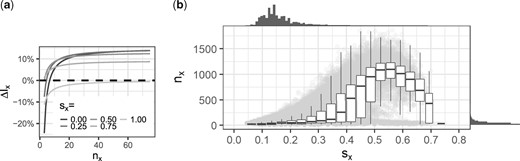
(a) $\Delta I_x$ as a function of n_x, for various values of s_x. (b) The distributions of and dependencies between s_x and n_x on the real data. We use a random subsample of 1 mil bit positions for the plot, but omit those positions that are determined at the root (i.e. n_x = 1). These make up 15% of all values, and they all have s_x = 0. Each of the remaining positions are shown as a gray dot in the background. The s_x values are binned and the distribution of n_x within each bin is shown as a box plot. On the top (respectively, right) of the plot is the histogram of s_x (respectively, n_x)

In large scale applications, our theoretical analysis can be simplified by assuming that n_x goes to the limit. However, HowDe-SBT can be applied in different settings, and some of these settings (like a private patient cohort) may in fact not be very large. Our detailed analysis can be used to determine at which point a dataset is large enough for the asymptotic effects to kick in; e.g. Figure 3a indicates that the space savings reaches a stable point roughly at n_x = 50.

We caution, however, that our analysis does not automatically translate to total improvements when all the positions are considered jointly. The total data structure size depends a lot on the structure of the input. That is reflected by the distribution of n_x and s_x in the real data, whether or not they are correlated, the entropy of all the bits together, rather than separated by position and the higher-order entropy of the bitvectors. These effects can be analyzed using real data, which we do in Section 6.

5 Construction algorithm

In this section, we describe an algorithm to compute $B_{\text{det}}^{\text{sqz}\hspace{0.17em}}$ and $B_{\text{how}}^{\text{sqz}\hspace{0.17em}}$ for a given topology and prove its correctness. Our algorithm makes a pass through the tree using a post-order traversal. At each node u, it (i) computes B_det and B_how of u, and (ii) computes $B_{\text{det}}^{\text{sqz}\hspace{0.17em}}$ and $B_{\text{how}}^{\text{sqz}\hspace{0.17em}}$ of each of its children using their B_det and B_how. As the final step, $B_{\text{det}}^{\text{sqz}\hspace{0.17em}}$ and $B_{\text{how}}^{\text{sqz}\hspace{0.17em}}$ are computed for the root node.

The base case of the algorithm is, for each leaf u, to set $B_{\text{det}}(u)\leftarrow \xi$ and $B_{\text{how}}(u)\leftarrow B_{\cup }(u)$⁠. For an internal node u, we first construct $B_{\cap }(u)$ and $B_{\cup }(u)$ using the operations:

$$\begin{array}{c}{B}_{\cap }(u)\leftarrow \bigcap _{c\in \text{children}(u)}{B}_{\text{how}}\hspace{0.17em}(c)\\ B_{\cup }(u)\leftarrow \bigcup _{c\in \text{children}(u)}\left(\overline{B_{\text{det}}(c)}\cup B_{\text{how}}(c)\right)\end{array}$$

Then, $B_{\text{det}}(u)$ and $B_{\text{how}}(u)$ are constructed by directly applying their definitions (Equation 1). Once $B_{\text{det}}(u)$ and $B_{\text{how}}(u)$ have been computed, we compute the active bits in $B_{\text{det}}(c)$ and $B_{\text{how}}(c)$⁠, for each child c of u:

$$B_{\text{det}}^{\text{active}\hspace{0.17em}}(c)\leftarrow \overline{B_{\text{det}}(u)}\hspace{0.17em}\hspace{0.17em}\hspace{0.17em}\hspace{0.17em}\hspace{0.17em}\hspace{0.17em}\hspace{0.17em}\hspace{0.17em}\hspace{0.17em}\hspace{0.17em}\hspace{0.17em}\hspace{0.17em}\hspace{0.17em}{B}_{\text{how}}^{\text{active}\hspace{0.17em}}(c)\leftarrow B_{\text{det}}(c)\cap \overline{B_{\text{det}}(u)}$$

Next, we make a linear scan through $B_{\text{det}}(c)$ and $B_{\text{how}}(c)$ and copy over only the bits that are set in $B_{\text{det}}^{\text{active}\hspace{0.17em}}(c)$ and $B_{\text{how}}^{\text{active}\hspace{0.17em}}(c)$⁠, respectively, thus generating $B_{\text{det}}^{\text{sqz}\hspace{0.17em}}(c)$ and $B_{\text{how}}^{\text{sqz}\hspace{0.17em}}(c)$⁠.

These are finally RRR compressed and written to disk.

After the post-order traversal completes, we make the final step to compute the $B_{\text{det}}^{\text{sqz}\hspace{0.17em}}$ and $B_{\text{how}}^{\text{sqz}\hspace{0.17em}}$ for the root u. It is essentially the same process as for the internal nodes, but the active bits are set as:

$$B_{\text{det}}^{\text{active}\hspace{0.17em}}(u)\leftarrow \xi \hspace{0.17em}\hspace{0.17em}\hspace{0.17em}\hspace{0.17em}\hspace{0.17em}\hspace{0.17em}\hspace{0.17em}\hspace{0.17em}\hspace{0.17em}\hspace{0.17em}\hspace{0.17em}\hspace{0.17em}\hspace{0.17em}\hspace{0.17em}\hspace{0.17em}\hspace{0.17em}\hspace{0.17em}\hspace{0.17em}\hspace{0.17em}\hspace{0.17em}{B}_{\text{how}}^{\text{active}\hspace{0.17em}}(u)\leftarrow B_{\text{det}}(u)$$

$B_{\text{det}}^{\text{sqz}\hspace{0.17em}}$ and $B_{\text{how}}^{\text{sqz}\hspace{0.17em}}$ are then computed as before, removing the inactive bits during a linear scan followed by RRR compression.

We note that the B_∪, B_∩, B_det,  B_how,  $B_{\text{det}}^{\text{active}\hspace{0.17em}}$ and $B_{\text{how}}^{\text{active}\hspace{0.17em}}$ bitvectors are not stored after construction is complete. To save memory, these can be discarded right after their use; however, it is necessary to save some of the B_det and B_how vectors. Specifically, we must save $B_{\text{det}}(u)$ and $B_{\text{how}}(u)$ between the visit to u and the visit to u’s parent. During this interval they can be saved in memory or, in order to save memory, they can be written to disk and reloaded to memory as needed (the default behavior). When u’s parent is visited, $B_{\text{det}}^{\text{sqz}\hspace{0.17em}}(u)$ and $B_{\text{how}}^{\text{sqz}\hspace{0.17em}}(u)$ are computed and $B_{\text{det}}(u)$ and $B_{\text{how}}(u)$ are no longer needed.

The following theorem shows that our algorithm is correct and that its runtime is linear in the total size of the input bitvectors. 

Theorem 3. Given a database of n BFs, each of size b and a tree topology, our method constructs $B_{\text{det}}^{\text{sqz}\hspace{0.17em}}$ and $B_{\text{how}}^{\text{sqz}\hspace{0.17em}}$ for all nodes in $\mathcal{O}(\mathit{nb})$ time.

Proof. We first prove the runtime. Our bitvector construction algorithm operates on each node twice—once when the node is visited, and a second time to finish the node when its parent is visited. (The root is a special case—its finishing stage occurs at the end of the algorithm.) At each stage, it performs a constant number of bitwise operations which each takes $\mathcal{O}(b)$ time. Similarly, the linear scan to remove inactive bits can be done in $\mathcal{O}(b)$ time by simply copying the active bits to a new vector.

Next, we prove correctness. We will need the following technical lemma: 

Lemma 1. The following properties are true:

$$B_{\cap }(u)=B_{\cup }(u)\hspace{1em}\hspace{1em}\hspace{1em}\hspace{1em}\mathrm{if}\hspace{0.17em}\hspace{0.17em}u\hspace{0.17em}\hspace{0.17em}\mathrm{is}\hspace{0.17em}\hspace{0.17em}\mathrm{a}\hspace{0.17em}\hspace{0.17em}\text{leaf}$$

(4)

 

$$B_{\cup }(u)=\overline{B_{\text{det}}(u)}\cup B_{\text{how}}(u)$$

(5)

Proof. Equation (4) trivially follows from the definition of B_∩. For Equation (5), first observe that $B_{\cap }(u)$ and $\overline{B_{\cup }(u)}$ are disjoint (since $B_{\cap }(u)\subseteq B_{\cup }(u)$⁠). Combine this with the definition of $B_{\text{det}}(u)$⁠, and we get $\overline{B_{\cup }(u)}=B_{\text{det}}(u)\setminus B_{\cap }(u)=B_{\text{det}}(u)\cap \overline{B_{\cap }(u)}$⁠. Negating both sides, we get $B_{\cup }(u)=\overline{B_{\text{det}}(u)}\cup B_{\cap }(u)=\overline{B_{\text{det}}(u)}\cup B_{\text{how}}(u)$ □

We first show the correctness of computing B_det and B_how when we visit u. For a leaf u,

$$\begin{array}{cc}{B}_{\text{det}}(u)=B_{\cap }(u)\cup \overline{B_{\cup }(u)}& \text{\hspace{1em}\hspace{1em}(by definition)}\\ =B_{\cup }(u)\cup \overline{B_{\cup }(u)}& [\text{from Equation (4)]}\\ =\xi & \end{array}$$

 

$$\begin{array}{cc}{B}_{\text{how}}(u)=B_{\cap }(u)\hfill & \text{\hspace{1em}\hspace{1em}(by definition)}\\ =B_{\cup }(u)& [\text{from Equation }(4)]\end{array}$$

If u is an internal node, then it is enough to show that B_∩ and B_∪ are computed correctly.

$$\begin{array}{cc}{B}_{\cap }(u)={\displaystyle \bigcap _{c\in \text{children}(u)}{B}_{\cap }}(c)& \text{(by definition)}\\ ={\displaystyle \bigcap _{c\in \text{children}(u)}{B}_{\text{how}}}(c)& (\text{from\hspace{0.17em}\hspace{0.17em}def}.\text{\hspace{0.17em}\hspace{0.17em}of\hspace{0.17em}\hspace{0.17em}}{B}_{\text{how}})\end{array}$$

 

$$\begin{array}{cc}{B}_{\cup }(u)={\displaystyle \bigcup _{c\in \text{children(}u)}{B}_{\cup }}(c)& \text{\hspace{1em}\hspace{1em}(by definition)}\\ ={\displaystyle \bigcup _{c\in \text{children}(u)}\left(\overline{B_{\text{det}}(c)}\cup B_{\text{how}}(c)\right)}& \text{\hspace{0.17em}[from Equation (5)]}\end{array}$$

To show the correctness of computing $B_{\text{det}}^{\text{active}\hspace{0.17em}}(c)$ and $B_{\text{how}}^{\text{active}\hspace{0.17em}}(c)$⁠, recall their definitions from Section 3. It is straightforward to see that our algorithm computes $B_{\text{det}}^{\text{active}\hspace{0.17em}}$ and $B_{\text{how}}^{\text{active}\hspace{0.17em}}$ exactly according to these definitions, both for the case of children and for the case of the root. Finally, the algorithm correctly computes $B_{\text{det}}^{\text{sqz}\hspace{0.17em}}$ and $B_{\text{how}}^{\text{sqz}\hspace{0.17em}}$ because it simply applies their definitions. □

We note that the complexity of constructing the tree topology was not studied in Sun et al. (2018), but the obvious implementation would take $\Omega (n^2)$ time. Though it takes negligible time on currently tested datasets, it may become the bottleneck in the future if n increases by several orders of magnitude.

6 Results

6.1 Experimental setup

To evaluate HowDe-SBT, we compared it against its two predecessors, AllSome-SBT (Sun et al., 2018) and SSBT (Solomon and Kingsford, 2017). All experiments were run on an Intel Xeon CPU with 512 GB of RAM and 64 cores (at 2.10 GHz). Our tool is open source and available for free through https://github.com/medvedevgroup/HowDeSBT. All details about how the tools were run, including parameters, together with datasets needed to reproduce our results, are available on https://github.com/medvedevgroup/HowDeSBT/tree/master/reproduce.

We used the same data for evaluation as Solomon and Kingsford (2016), except that we removed experiments that did not have reads longer than k. There were 66 experiments removed in this way. A 67th experiment was removed because the corresponding BF in Solomon and Kingsford (2016) was empty. Together, the removed experiments had a total of 675 million reads. The resulting dataset contained 2585 human RNA-seq runs from blood, brain and breast tissues, compromising all relevant human RNA-seq datasets in the SRA at the time of Solomon and Kingsford (2016). For each file, we filtered out any k-mers that occurred less than a file-dependent threshold. We used the thresholds from Pandey et al. (2018), for consistency purposes. We used k = 20 and a BF size of $b=2·{10}^9$ (as in previous work) and k-mer counting was done using Jellyfish (Marçais and Kingsford, 2011).

To study query performance, we created four types of queries: a single transcript, a batch of 10 transcripts, a batch of 100 and a batch of 1000. Transcripts were picked arbitrarily from Gencode (ver. 25) transcripts that are at least k nt long. We created 100, 10, 3 and 3 replicates for each type of query, respectively. We include batches of multiple transcripts in our tests because SBT performance is known to depend on batch size (Solomon and Kingsford, 2016). The idea of combining multiple queries in a batch and then processing them at each node simultaneously was first described by Solomon and Kingsford (2016) and is implemented in all SBT methods, including HowDe-SBT. We use a value of $\theta =0.9$ for all experiments. Note that because the output of HowDe-SBT is identical to SSBT and AllSome-SBT, we do not need to compare their accuracy; moreover, a comparison of SBT accuracy relative to exact methods like Mantis was also already explored in Solomon and Kingsford (2016).

6.2 Performance comparison

Table 1 shows the time and space taken to construct the index. The index could be created in less than 36% of the time and with 39% less space for HowDe-SBT than for all other approaches. The faster construction time of HowDe-SBT over AllSome-SBT was due to a combination of having to handle much smaller bitvectors during construction (as reflected by the smaller index size) and software engineering improvements. Otherwise, the construction algorithms of the two methods differ only by the specific bitvector operations applied during the tree traversal.

Table 1.

File sizes (in GiB) and build times

	HowDe-SBT	AllSome-SBT	SSBT
Construction time (h)	9	25	57
Intermediate space	602	602	602
Index size	14	142	23

Notes: The intermediate space refers to the initial experiment BFs. The construction time is the time to build the index from the BFs and does not include k-mer counting. All times shown are on one processor.

It is important to note that the construction times in Table 1 do not include the pre-processing time of converting the SRA read files to the initial experiment BFs. This is a time-consuming process, which took us several days using multiple threads. We did not obtain reliable timing results since we did the conversion on the fly while streaming the data from the SRA over a network connection.

To measure the query time, we first note that there are different use cases that effect how to best measure time performance. SBT approaches are designed to scale to a very large number of experiments or to machines with limited memory (e.g. a desktop computer) because the memory required for a query is not dependent on the number of experiments; only one node of the tree needs to be loaded into memory at any given time. Therefore, we focused our analysis on a setting where the index is loaded into memory with each new query.

Table 2 shows the query speed for all tools. HowDe-SBT was faster than other SBT approaches, with over a 5x speedup on single-transcript batches. Peak RAM usage was < 1.3 GiB for all batches for all tools Table 3.

Table 2.

Query times (s)

	HowDe-SBT	AllSome-SBT	SSBT
Single	5.4	36.7	29.4
Ten	44.5	353.7	159.6
Hundred	171.3	817.8	400.8
Thousand	719.7	1168.6	3509.4

Notes: Values shown are the median over all the replicates. The cache was cleared prior to each run.

Table 3.

Peak resident RAM (in GiB) observed during queries

	HowDe-SBT	AllSome-SBT	SSBT
Single	0.8	0.3	1.3
Ten	0.8	0.3	1.1
Hundred	0.8	0.3	1.1
Thousand	0.8	0.6	1.1

Note: Values shown are the maximum over all the replicates.

We also tested the effect of warming the cache prior to querying, where we ran each query two consecutive times and then reported the run-time for the second run (Supplementary Table S1). Warming the cache prior to querying led to improved query times for all tools, but their relative performance remained mostly similar.

6.3 Bitvector properties

First, we investigate how many positions are active and how saturated the active bits are. The fraction of active B_det positions decreases going down the tree (by definition), with a median of 0.006 at internal nodes and 0.002 at leaves. The saturation of $B_{\text{det}}^{\text{sqz}\hspace{0.17em}}$ (i.e. the percentage of the active bits that are determined) is 100% at the leaves (by definition) and has a median of 41% at the internal nodes. The saturation of $B_{\text{how}}^{\text{sqz}\hspace{0.17em}}$ (i.e. the percentage of the active B_how bits that are 1) has a median of 51% at the leaves and 12% at the internal nodes. It decreases with the height of a node (i.e. maximum distance to a leaf), meaning that at higher levels of the tree, the vast majority of positions that are determined are found to be absent rather than present. Figure 4 shows the saturation distributions. In terms of final space on disk, after RRR compression, the leaves account for only 18% of the total index size.

Fig. 4.

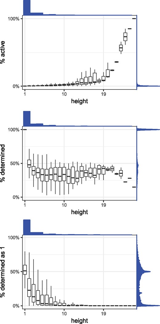
The distribution of nodes’ bitvector saturations, as a function of a node’s height (i.e. maximum distance to a leaf). The top panel shows barplots for the percentages of positions in the B_det vector that are active, the middle panel shows barplots for the percentages of those positions that are set to 1 (i.e. determined) and the bottom panel shows barplots for the percentages of active B_how positions that are set to 1. Above each plot is the histogram of height values, and to the right of each plot is the density plot of the percentages being measured in that plot

In Section 4, we derived the reduction in space and query time for a bit position x in terms of the number of nodes where it is active in B_det (denoted by n_x) and the fraction of nodes where it is set to one in B_how (denoted by s_x). Figure 3b shows the distribution of these values on our tree. The median value for s_x is 0.14 and for n_x is 31, which corresponds to $\Delta I_x\approxeq 14\%$ in Figure 3a. However, we also see a correlation between n_x and s_x (Spearman coefficient of r = 0.67). Any future extension of our theoretical analysis per bit position to one of all bit positions jointly should take this complexity into account. We note that the total reduction in index size of HowDe-SBT over SSBT on our data (38%) is due not only to the improved bit representation but also due to the better tree topology that HowDe-SBT constructs; thus, a direct comparison to our theoretical predictions is challenging.

7 Conclusion

In this paper, we presented a novel approach for the representation of SBTs and studied its performance from both a theoretical and an experimental perspective. The main intuition behind our representation is that it reduces the number and entropy of the active bits. Compared to previous SBT approaches, HowDe-SBT is an improvement on all fronts: it constructs the index in less than 36% of the time and with 39% less the space, and can answer small-batch queries five times faster. Compared specifically against AllSome-SBT, the biggest advantage is that the size of the index is an order of magnitude smaller. In comparison against SSBT, the biggest advantage is in the construction time and query times, across all batch sizes.

With the improvements in this paper, the SBT can already be deployed for small and mid-size databases, such as a private patient cohort or all the sequencing data in flybase.org. Such a deployment will need to provide an automated way to update the database; while our method naturally supports insertions in $\mathcal{O}(\text{height}·b)$ time [we have omitted the details, but Sun et al. (2018) give the basic overview of how insertions can be handled], a quality assurance step will be necessary prior to automating database updates. It will also be necessary to provide a front-end interface [e.g. Galaxy or similar to Bradley et al. (2017)]) for easy access. Such front-ends should also provide wrappers for more biologically-oriented queries (i.e. to convert ‘which sample has a SNP’ into a k-mer query).

Acknowledgements

The authors are thankful to Ayaan Hossain and Natasha Stopa for helping prototype some aspects of this project. This work has been supported in part by NSF awards DBI-1356529, CCF-551439057, and IIS-1453527 to PM and partially supported by PSU’s College of Engineering Multidisciplinary Seed Grant Program. Research reported in this publication was supported by the National Institute Of General Medical Sciences of the National Institutes of Health under Award Number R01GM130691. The content is solely the responsibility of the authors and does not necessarily represent the official views of the National Institutes of Health.

Conflict of Interest: none declared.