Automatic local resolution-based sharpening of cryo-EM maps

Abstract

Motivation

Recent technological advances and computational developments have allowed the reconstruction of Cryo-Electron Microscopy (cryo-EM) maps at near-atomic resolution. On a typical workflow and once the cryo-EM map has been calculated, a sharpening process is usually performed to enhance map visualization, a step that has proven very important in the key task of structural modeling. However, sharpening approaches, in general, neglects the local quality of the map, which is clearly suboptimal.

Results

Here, a new method for local sharpening of cryo-EM density maps is proposed. The algorithm, named LocalDeblur, is based on a local resolution-guided Wiener restoration approach of the original map. The method is fully automatic and, from the user point of view, virtually parameter-free, without requiring either a starting model or introducing any additional structure factor correction or boosting. Results clearly show a significant impact on map interpretability, greatly helping modeling. In particular, this local sharpening approach is especially suitable for maps that present a broad resolution range, as is often the case for membrane proteins or macromolecules with high flexibility, all of them otherwise very suitable and interesting specimens for cryo-EM. To our knowledge, and leaving out the use of local filters, it represents the first application of local resolution in cryo-EM sharpening.

Availability and implementation

The source code (LocalDeblur) can be found at https://github.com/I2PC/xmipp and can be run using Scipion (http://scipion.cnb.csic.es) (release numbers greater than or equal 1.2.1).

Supplementary information

Supplementary data are available at Bioinformatics online.

1 Introduction

The application of Cryo-Electron Microscopy (cryo-EM) to structure determination relies on the quality of reconstructed EM density maps to enable accurate construction of atomic models. As such, methodological advancements that enhance the map quality can play a significant role in the reliability of the resulting atomic models. Addressing this problem, the so-called sharpening methods have recently been introduced in cryo-EM workflows as a post-processing step, after being in common use in X-ray crystallography for a much longer time (Bass et al., 2002; Jacobson et al., 1961). In cryo-EM, the most widely applied method is a structure factor modification based on the Guinier plot, also known as B-factor correction (Rosenthal and Henderson, 2003). The general idea behind this approach is to overcome the loss of contrast at high resolution by boosting the amplitudes of structures factors in that resolution range, described by the ‘B-factor’, the slope of the amplitude falloff that will be boosted.

Sharpening algorithms can coarsely be classified as global and local. However, to our knowledge, all of them make use of the basic amplitude correction method introduced above. Thus, global sharpening determines a B-factor value, which is then applied across the whole map. RELION post-processing (Scheres, 2015) belongs to this group, directly working on the Guinier plot, as newer methods, such as AutoSharpen in the Phenix Package (Terwilliger et al., 2018), also do; this latter method looks for a B-factor that maximizes the connectivity and minimizes the isosurface area of the cryo-EM map. Global approaches apply the same transformation to the whole map, neglecting the fact that different regions might present different resolutions. In contrast, in the local sharpening group, LocScale (Jakobi et al., 2017) compares the radial average of the structure factors inside both a moving window of the experimental map and of the map calculated from the corresponding atomic model. Then, it locally scales the map amplitudes in Fourier space to be in agreement with the atomic model. An obvious shortcoming of this method, of course, is the essential requirement for a starting atomic model, which may restrict its applicability.

To overcome the limitations above, a fully automatic and virtually parameter-free local sharpening method based on local resolution estimation is presented in this work. The algorithm, named LocalDeblur, acts via local deblurring. Our method solves the sharpening problem using a gradient descent version of the Wiener filter. The root of this algorithm is a space-varying filter. We consider that the observed cryo-EM density map has been obtained by the convolution with a local, lowpass filter whose frequency cutoff is given by the local resolution estimate. We compute the sharpened map with an iterative steepest descent method. LocalDeblur does not require an atomic model and, consequently, is bias free in this regard. Full derivation of LocalDeblur is presented in Section 2.

2 Materials and methods

2.1 Local deblurring method (LocalDeblur)

Consider two density maps $v_{\mathrm{sh}}$ and $v_{\mathrm{obs}},$ respectively, called sharpened and observed, such that $v_{\mathrm{obs}}$ is a degraded reconstruction map obtained from $v_{\mathrm{sh}}$ as

$$v_{\mathrm{obs}}=H{v}_{\mathrm{sh}}$$

The volumes are represented by vectors in lexicographic order and H is a blurring operator responsible for degrading the sharpened map. More details on the nature of the matrix H can be found in Supplementary Material. There would many ways to model H, and in this work, we have chosen to define H as a local filter constructed by applying a filter bank upon the map $v_{\mathrm{sh}}$⁠. Each filter in the bank is a bandpass raised cosine filter centered at frequency ${\omega }_i$ (corresponding to a resolution ${{\omega }_i=1/R}_i$⁠), see Supplementary Material, and represented by matrix $H^i$⁠. In this way, the local filter is constructed by the addition of many bandpass filters with different weights covering the frequency range up to the maximum resolution determined for the input map (i.e. beyond the local resolution at a specific point, all filters contribute with zero weight at that particular location) and distributed every 0.2 Å of resolution. Each channel in the filter bank is locally weighted according to the difference between the local resolution, $R_{\mathrm{local}}$⁠, and the spatial frequency of the center of each bandpass filter ${\omega }_i$ (⁠${\mathrm{ }R}_i=1/{\omega }_i$⁠). Note that $R_{\mathrm{local}}$ is another vector of the same size as the input map, whose $j$th entry is the estimate of the local resolution at the $j$th location. We get these estimates of local resolution using MonoRes (Vilas et al., 2018). The local weight is given by a diagonal matrix, $W^i$⁠, whose $(j,\mathrm{ }j)$th entry is

$$w_{\mathit{jj}}^i=e^{-K{(R_{\mathrm{local},j}-R_i)}^2}$$

Empirically, we have observed that $K=0.025$ casts good results for all tests we performed. In general, values ranging between 0.01 and 0.05 can be used without detecting large differences. Specifically for low resolution maps (<6 Å), 0.01 is a good choice. This weight matrix tends to favor the contribution of voxels to the frequencies associated to their local resolution, while still including low and medium resolution components (in fact, it is like a very broad bandpass filter, with maximum at the local resolution). Therefore, the matrix H can be mathematically written as:

$$H={\left(\sum _i\mathrm{ }{W}^i\right)}^{-1}\left(\sum _i\mathrm{ }{W}^i{H}^i\right)$$

Note that the inverse matrix in front must be introduced as a normalization term in the filter. However, due to its diagonal nature, it is trivial to invert this matrix.

Our method solves the sharpening problem using a gradient descent version of the Wiener filter. For completeness, let us succinctly give, here, a short derivation of it. The Wiener filter can be regarded as the solution of a Bayesian restoration problem in which the noise and the signal both follow multivariate Gaussian distributions with zero means and covariance matrices ${\mathrm{\Sigma }}_n$ and ${\mathrm{\Sigma }}_x$ (Mackay, 2004). The Maximum a posteriori estimate of the signal would be given by

$${\mathit{v}}_{\mathrm{sh}}^{\mathrm{*}}={\mathrm{argmin}}_{v_{\mathrm{sh}}}E\left(v_{\mathrm{sh}}\right)={\mathrm{argmin}}_{v_{\mathrm{sh}}}\{-\ln P\left({\mathit{v}}_{\mathrm{obs}}|v_{\mathrm{sh}}\right)P\left(v_{\mathrm{sh}}\right)\}$$

(1)

$$={\mathrm{argmin}}_{v_{\mathrm{sh}}}\{{\left(v_{\mathrm{obs}}-\mathrm{H}{v}_{\mathrm{sh}}\right)}^T{\mathrm{\Sigma }}_n^{-1}\left(v_{\mathrm{obs}}-H{v}_{\mathrm{sh}}\right)+{v_{\mathrm{sh}}}^T{\mathrm{\Sigma }}_x^{-1}{v}_{\mathrm{sh}}\}$$

This optimization problem can be easily solved by steepest descent approach

$$v_{\mathrm{sh}}^{(j+1)}=v_{\mathrm{sh}}^{\left(j\right)}+\lambda \left(H^T{\mathrm{\Sigma }}_n^{-1}\left(v_{\mathrm{obs}}-H{v}_{\mathrm{sh}}^{\left(j\right)}\right)-{\mathrm{\Sigma }}_x^{-1}{v}_{\mathrm{sh}}^{\left(j\right)}\right)$$

(2)

with $v_{\mathrm{sh}}^{\left(0\right)}=v_{\mathrm{obs}}$ (Sorzano et al., 2017). Note that we are explicitly doing an approximation by assuming a very simple form of the signal covariance matrix of the form$\mathrm{ }{\mathrm{\Sigma }}_x={\sigma }_x^{2}I$⁠, i.e. each voxel is independent of the rest. We acknowledge that this is a limiting assumption and that, furthermore, some very specific software—like RELION—addresses this calculation directly; however, this is not the case for other reconstruction software and we wanted to make our new method suitable for any 3D reconstruction algorithm. Under these considerations, the Gaussian prior for the signal results in the usual Tikhonov regularization term and, this iteration can be written as

$$v_{\mathrm{sh}}^{(j+1)}=v_{\mathrm{sh}}^{\left(j\right)}+\lambda \left(H^T\left(v_{\mathrm{obs}}-H{v}_{\mathrm{sh}}^{\left(j\right)}\right)-\frac{1}{\mathrm{SNR}}{v}_{\mathrm{sh}}^{\left(j\right)}\right)$$

where the SNR is the signal-to-noise ratio defined as $\mathrm{SNR}={\sigma }_x^2/{\sigma }_n^2$⁠. In our algorithm, ${\sigma }_x$ and ${\sigma }_n$ are calculated using a mask defining the regions corresponding to the signal and to the noise, respectively. When the SNR is high, the deblurring term dominates, while for low SNR, the regularization term dominates. As far as we know, the statistical distribution of noise in the reconstructed volumes has not been thoroughly studied. However, we know that the noise distribution at the level of projection images is Gaussian (Sorzano et al., 2004), which makes the Gaussian assumption at the level of volumes plausible (although non-white due to the contrast transfer function of the images, the Fourier spectrum of the noise and the local correlation induced by the 3D reconstruction algorithm). We realize that the assumption of Gaussian and independent distribution for the reconstructed volume ${\mathrm{\Sigma }}_x$ is a much stronger simplification that is actually not met by macromolecules (Sorzano et al., 2015). However, this assumption allows the derivation of a simple, iterative algorithm (other distributions would result in much more complicated iterations). We have further reduced the complexity by working only with an approximate value of the variance of each coefficient in the volume, which is an easily estimated number, instead of the true underlying covariance matrix, which would be seldom known by the user. We acknowledge that these assumptions correspond to theoretical limitations of our approach that make it only approximate; however, stated in this manner, the problem leads to a practical and easy to apply solution whose application to a varied set of experimental cases has been shown to produce much improved results.

It can be easily shown that the standard Wiener solution

$$v_{\mathrm{sh}}^{\left(\mathrm{Wiener}\right)}={\mathrm{\Sigma }}_x{H}^T{\left(H{\mathrm{\Sigma }}_x{H}^T+{\mathrm{\Sigma }}_n\right)}^{-1}{v}_{\mathrm{obs}}$$

(3)

is a fixed point of our iterations. To confirm this premise, we define $D=H{\mathrm{\Sigma }}_x{H}^T+{\mathrm{\Sigma }}_n$ and then study the gradient of the function of Eq. (1) at $v_{\mathrm{sh}}^{\left(\mathrm{Wiener}\right)}$

$$\nabla E\left(v_{\mathrm{sh}}^{\left(\mathrm{Wiener}\right)}\right)=-2H^T{\mathrm{\Sigma }}_n^{-1}\left(v_{\mathrm{obs}}-H{v}_{\mathrm{sh}}^{\left(\mathrm{Wiener}\right)}\right)+{2\mathrm{\Sigma }}_x^{-1}{v}_{\mathrm{sh}}^{\left(\mathrm{Wiener}\right)}=-2H^T{\mathrm{\Sigma }}_n^{-1}\left(v_{\mathrm{obs}}-H{\mathrm{\Sigma }}_x{H}^T{D}^{-1}{v}_{\mathrm{obs}}\right)+{2\mathrm{\Sigma }}_x^{-1}{\mathrm{\Sigma }}_x{H}^T{D}^{-1}{v}_{\mathrm{obs}}\mathrm{ }=-2H^T\left({\mathrm{\Sigma }}_n^{-1}D-{\mathrm{\Sigma }}_n^{-1}H{\mathrm{\Sigma }}_x{H}^T-I\right)D^{-1}{v}_{\mathrm{obs}}$$

If we now substitute the definition of $D$ in the parenthesis, we obtain

$$\nabla E\left(v_{\mathrm{sh}}^{\left(\mathrm{Wiener}\right)}\right)=-2H^T\left({\mathrm{\Sigma }}_n^{-1}\left(H{\mathrm{\Sigma }}_x{H}^T+{\mathrm{\Sigma }}_n\right)-{\mathrm{\Sigma }}_n^{-1}H{\mathrm{\Sigma }}_x{H}^T-I\right)D^{-1}{v}_{\mathrm{obs} }=-2H^{T}0D^{-1}{v}_{\mathrm{obs}}=0$$

This small digression proves that our iterative algorithm in Eq. (2) converges to the Wiener solution in Eq. (3) (because the covariance matrices are positive definite and, consequently, the objective function is convex), with the advantage that it can be efficiently implemented in Fourier space. However, a direct implementation of Eq. (3) involves an inversion of a formidable matrix, which is computationally impractical. This iterative formula is repeated until a convergence criterion is reached. Our algorithm stops when the change between two successive iterations is <1%. The choice of the step size, $\lambda$⁠, should be enough small to guarantee the convergence, but also large enough to speed-up convergence. We have observed that the following step size is a good compromise between both objectives:

$$\lambda =\frac{\Vert v_{\mathrm{obs}}\Vert /\Vert \left(H{v}_{\mathrm{obs}}\right)\Vert }{10}$$

2.2 Implementation

The algorithm is publicly available from Xmipp (de la Rosa-Trevin et al., 2013) (http://xmipp.cnb.csic.es) and integrated in the image processing framework Scipion 1.2.1 (de la Rosa-Trevin et al., 2016) (http://scipion.cnb.csic.es). LocalDeblur accepts an unfiltered 3D reconstruction cryo-EM density map and a local resolution map calculated either with MonoRes (Vilas et al., 2018) or ResMap (Kucukelbir et al., 2014).

2.3 Application of other sharpening methods

A number of sharpening methods, such as RELION post-processing, Phenix AutoSharpen and LocScale were used for comparison purposes; we note that although more approaches may have been used in concrete cases, the comparison with these three sharpening methods largely covers the majority of cases found in the Electron Microscopy Data Base (EMDB; Lawson et al., 2016). AutoSharpen was applied with the default parameters, only taking into account the resolution reported in each case. For LocScale, each PDB model was aligned to its corresponding map and applied as described previously (Jakobi et al., 2017). For TRPV1, PDB ID: 3j5p was used and for the 80S ribosome PDBs ID: 3j79, 3j7a were used.

3 Results

The performance of LocalDeblur was tested in depth with five unsharpened cryo-EM density maps. Three maps came from the recent EMDB map challenge (Heymann et al., 2018): TRPV1 channel (EMD-5778) (Liao et al., 2013), Plasmodium falciparum 80S ribosome (EMD-2660) (Wong et al., 2014) and Thermoplasma acidophilum 20S proteasome (EMD-6287) (Campbell et al., 2015), while the other two maps were at lower resolution: bovine cytochrome bc1 (EMD-4288) (Amporndanai et al., 2018) and L-20S (NSF/αSNAP/L-SNARE) complex (EMD-8944) (Choi et al., 2018). Additionally, we have performed an analysis of the recent structure of an agonist-bound human calcitonin receptor Gs complex (CTR-Gs) (Liang et al., 2017). The local resolution needed for our algorithm was calculated using MonoRes (Vilas et al., 2018).

Naturally, all current methods for cryo-EM sharpening considerably enhance map interpretability. To establish the utility and relative performance of an automatic and parameter-free method such as the one presented in this work (especially relevant since it does not need to have a prior/initial structural model), we performed comparisons between LocalDeblur and current versions of the main sharpening methods in use in the field, specifically, RELION post-processing (Scheres, 2015), Phenix AutoSharpen (Terwilliger et al., 2018) and LocScale (Jakobi et al., 2017). Two sets of comparisons were performed, first was a direct analysis of the maps (Figs 1, 2, 4 and 5 and Supplementary Figs S1 and S2), and second, an analysis of their corresponding Guinier plots (Fig. 3 and Supplementary Fig. S3).

Fig. 1.

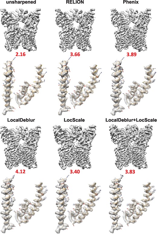
Sharpened map of TRPV1 (EMD-5778) generated with LocalDeblur and comparison with the main sharpening methods (RELION post-processing, Phenix AutoSharpen and LocScale). Below each map, the value of EMRinger score is shown and the densities corresponding to 419–456 (left) and 568–642 (right) residues are represented

3.1 Comparison of sharpening methods

Qualitatively, it can be clearly appreciated that all sharpened maps have more details than the original maps, and that in LocalDeblur maps the α-helical pitch is more clearly delineated and the density for most side chains is better defined than in the other methods, which can substantially facilitate the construction of the corresponding atomic model. The application to TRPV1 (Fig. 1) demonstrates the enhanced utility of LocalDeblur for membrane proteins, while 80S ribosome map (Supplementary Fig. S1) shows that LocalDeblur works very well with macromolecules that contain both amino acids and nucleotides. Indeed, LocalDeblur improves the contrast between these two features and allows a better definition of high-resolution features.

Next, we combined LocalDeblur and LocScale. The objective was to determine if the knowledge of an initial atomic model could further enhance the sharpened map by applying LocScale, once LocalDeblur had increased the interpretability of the map (without any additional information). This may be a way to reduce possible dependencies of any sharpening approach, making explicit usage of a model with the model itself, minimizing the probability of reaching local minima. Figures 1 and 3 and Supplementary Figs S1 and S3 present the results of this combination. As shown, if the atomic model of the EM map is available, a combination of LocalDeblur and LocScale may produce an even better sharpened map. However, this effect seems to be case dependent, being much clearer for the ribosome than for TRPV1. This experimental fact probably reflects that sharpening generated by methods requiring a prior structural model may be quite conditioned by such specific starting model, which may introduce some uncertainty and instability. LocalDeblur, instead, is already powerful enough to produce a very substantial enhancement of the map without this constraint.

To check the applicability of our method when the maps have lower than quasi-atomic resolution, the sharpening of maps corresponding to bovine cytochrome bc1 (Fig. 2) and L-20S (Supplementary Fig. S2), resolved at 4.4 and 7 Å, respectively, was performed. Note that in these cases the application of prior information in the form of a starting model would be either impossible or, at best, doubtful. The application of LocalDeblur to the cryo-EM map of bovine bc1 (Fig. 2) allowed us to identify areas of the structure that could not be determined by the other methods; for example, residues from Thr 222 to Val 228 of chain A (Fig. 2A) and residues from Arg 227 to Gly 234 of chain B (Fig. 2B), that were not resolved in the RELION or Phenix post-processed maps or the proposed atomic model.

Fig. 2.

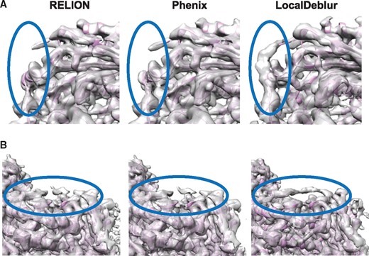
Sharpened maps of bovine cytochrome bc1 (EMD-4288). Two regions of the maps generated with RELION, Phenix and LocalDeblur are compared. Indicated areas highlight regions where LocalDeblur map shows densities allowing to trace the atomic model. (A) Area corresponding to the residues from Thr 222 to Val 228 of chain A. (B) Area corresponding to the residues from Arg 227 to Gly 234 of chain B

Extending this analysis, the LocalDeblur sharpening of L-20S complex showed that the method is also applicable for low resolution maps, substantially increasing their interpretability. However, in this case, in the absence of an available structural model, only qualitative judgments can be made with respect to map interpretability (Supplementary Fig. S2).

3.1.1 The map quality determines the quality of atomic model

We further quantitatively studied the influence of each of the sharpening methods compared in this work on the quality of the fitting of atomic models for the specific case of TRPV1. In this way, we refined the atomic model of TRPV1 (PDB ID: 3j5p) for each sharpened density map. The initial atomic model was fitted into the sharpened maps of TRPV1 using UCSF Chimera (Pettersen et al., 2004). Subsequently, the fitted model was further refined using Coot (Emsley and Cowtan, 2004) and, then, underwent five iterations of real-space refinement in Phenix (Adams et al., 2010), including rigid-body, model morphing, local real-space fitting, global gradient-driven and simulated annealing refinement. At the end of the refinement, we noticed that the quality of the geometrical parameters in every case is improved with respect to the ones of original model. For quantitative comparisons, EMRinger (Barad et al., 2015) values are shown under each map in Fig. 1, while other quality measures determined using MolProbity (Chen et al., 2010) are presented in Supplementary Table S1. The EMRinger score identifies the fraction of side chains whose corresponding density is rotameric. The highest EMRinger score within the transmembrane region is achieved for the refined atomic model with the LocalDeblur map, indicating that amino acid side chains are chemically realistic and fit very well into the density map.

3.2 Comparison of Guinier plots

The second set of comparisons addresses the behavior of structure factors as maps are sharpened by the different methods. In Fig. 3, we present the data corresponding to TRPV1 and, in Supplementary Fig. S3, those for the 80S ribosome, showing total coincidence. Focusing on TRPV1, the Guinier plot of the radially averaged profile of each sharpened map is presented, where the profile corresponding to the density map generated from the atomic model (PDB ID: 3j5p) is plotted with a dashed line. It is readily noticeable that this latter profile shows a decay and that it has a clear peak at ∼4.9 Å, which is within the range of characteristic distances of secondary structure elements (7–4 Å) (Morris et al., 2004). However, in the maps obtained with RELION post-processing and Phenix AutoSharpen, the characteristic features of the original structure factors at middle and high resolution are lost, including their frequency decay and the peak mentioned above. On the other hand, methods that take into account local characteristics of the maps (such as LocScale and LocalDeblur) are much more consistent with the expected structural factors corresponding to the structure under investigation. In general, local sharpening methods reproduce overall radial structure factor profiles much better than methods based on global B-factor. This fact correlates very well with the previous observation that secondary structure elements are substantially better presented in LocalDeblur than in any other method without prior information, even if the atomic model was not used at all in the calculations.

Fig. 3.

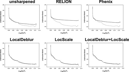
Guinier plots for each sharpened map represented in Fig. 1 are shown. The profile corresponding to the density map generated from the atomic model (PDB ID: 3j5p) is superimposed as a dashed line representing our ‘target result’. Note how profiles obtained by LocalDeblur are very similar to the target ones

All these experiments indicate that the application of global sharpening based on the B-factor value may not be an optimal procedure in cryo-EM. Indeed, owing to the intrinsic characteristics of the macromolecules and errors during the reconstruction workflow (Sorzano et al., 2001), different parts of the maps can have varying resolutions (Cardone et al., 2013; Kucukelbir et al., 2014; Vilas et al., 2018) and, consequently, they may require different levels of sharpening/blurring for optimal interpretation. In these cases, the selection of an appropriate global sharpening/blurring B-value becomes an impossible task, since it does not take into account the local SNR of the maps. A simple example is the proteasome core (EMD-6287) (Fig. 4), a ‘classic’ example in cryo-EM of a stable specimen. Indeed, the local resolution map determined with MonoRes (Vilas et al., 2018) indicates a relatively narrow range of local resolution values at the center, but with very significant degradations especially in the distal peripheral regions. Clearly, even for this ‘stable’ specimen, a global B-factor-based sharpening method would not be adequate to correctly analyze the density map corresponding to these lower resolution regions (Fig. 4B).

Fig. 4.

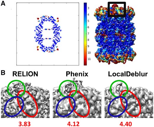
MonoRes results and sharpened maps of T. acidophilum 20S proteasome (EMD-6287). (A) MonoRes resolution slice and resolution map for the 20S proteasome. The black frame corresponds to the density enlarged in panel B. (B) Closed-up of the density maps generated with RELION post-processing, Phenix autosharpen and LocalDeblur, respectively, displaying the peripheral proteasome fragment marked in (A). Below each map, the EMRinger score for the refined model is shown in each case (using PDB ID: 6bdf). Note how LocalDeblur map is better defined in the indicated areas

3.3 Analysis of deblurring results on CTR-Gs

G protein-coupled receptors (GPCRs) are highly dynamic membrane proteins (Hilger et al., 2018). The first GPCR structure to be solved by cryo-EM was the calcitonin receptor (CTR) in complex with the peptide agonist salmon CT and transducer protein (heterotrimeric Gs). This initially published complex had a global resolution of 4.1 Å but exhibited substantial variance in local resolution (Liang et al., 2017). Later on, using additional data, the same macromolecule was further refined to a global resolution of 3.3 Å (dal Maso et al., 2019), and a new tracing was presented where relevant updates were reported. In this section, we have worked with the initial structure at 4.1 Å only and, together with the authors of the two works on CTR-Gs, we have shown how LocalDeblur applied to the initial data would have allowed the correct tracing of the polypeptide chain even without using the new 3.3-Å resolution data (dal Maso et al., 2019).

Indeed, analysis of the 4.1 Å CTR-Gs complex map following sharpening with LocalDeblur revealed two regions where the original deposited model (PDB ID 5UZ7) clearly contradicts the LocalDeblur-sharpened map, but not the deposited map sharpened in RELION. Further investigation, including structural alignment to the closely related CGRP receptor (Liang et al., 2018), and the availability of recently determined higher resolution CTR-Gs maps (dal Maso et al., 2019) revealed that regions within transmembrane helix 6 (TM6) and extracellular loop 2 (ECL2) were incorrectly modeled. In particular, L351 was misplaced within the TM6 kink induced by the conserved PXXG motif, resulting in a shift of the α-helical pitch (Fig. 5, upper panel), whereas the backbone of ECL2 was modeled into a region of poorly resolved density (Fig. 5, lower panel). The higher quality of the LocalDeblur maps and, in particular, enhanced connectivity and stronger signal at Cɑ atoms, made this kind of modeling errors especially obvious. Quantitatively, an improvement in the EMRinger score is also observed after application of LocalDeblur, as expected.

Fig. 5.

Sharpened maps from RELION post-processing (EMD-8623) and LocalDeblur of TM6 (upper panel) and ECL2 (lower panel) from the original work of Liang et al. (2017) are presented. The left-hand panels illustrate the original deposited EMD map (8623) and PDB model (5UZ7). The middle panels illustrate the LocalDeblur map with the original model. The right-hand panels illustrate the LocalDeblur map with remodeled protein that has been cross-validated with higher resolution maps. Below the corresponding EMRinger scores for the results before and after application of LocalDeblur are shown. Note that the LocalDeblur map is better defined in both regions, allowing for a more accurate modeling of the protein

4 Discussion

In this paper, we have introduced a new method to locally sharpen cryo-EM maps. The concepts behind our algorithm are straightforward; understanding the local resolution as a local blurring of an accurate map called sharpened map, which establishes a simple locally varying convolution relation between the measured and sharpened map via local resolution. The sharpened map is then obtained by an inversion of this operation. Indeed, the new method is automatic, parameter-free and only requires an estimate of the local resolution. Specifically, it does not need any initial structural model.

Results for different types of macromolecules have been used to test the algorithm. In particular, test cases were carefully chosen to cover many important scenarios, namely, membrane proteins (TRPV1 and CTR), high resolution volumes (proteasome), maps with broad resolution ranges (80S ribosome) and lower resolution maps (bovine cytochrome bc1 and L-20S). In all cases, LocalDeblur demonstrates excellent performance in comparison with other methods, improving the interpretability of the maps and increasing the fitting quality of an atomic model. Additionally, in those cases, in which the results of LocalDeblur have been compared with the Guinier plot arising from a known structural model, they have proven to be very similar, which is remarkable considering that LocalDeblur does not use any information from the structural model. Although the sharpening problem is approached using an iterative method, the results can be obtained in the range of minutes. For example, in a standard laptop, using 8 threads and the actual EMDB maps, the run time for TRPV1 is approximately 4 min, while for the proteasome is 7 min.

Moreover, to our knowledge, LocalDeblur is the first local sharpening approach combining the capacity to work in the absence of any prior structural model, the explicit use of local resolution estimations and the avoidance of global high frequencies boosting based on B-factor correction.

Author Contributions

J.M.C., C.O.S.S. and J.V. conceived the idea for this study. E.R.-A and J.L.V. wrote the code and the implementation in Scipion. P.C. and D.M. helped in the implementation in Scipion. E.R.-A designed the experiments and refined models. R.M. helped in the experiments and their interpretation. M.M. and R.M. helped in refined models. A.G. and P.M.S. refined and analysed the model for the CTR map. E.R.-A, J.L.V., J.M.C. and C.O.S.S. wrote the manuscript. All authors commented on and edited the manuscript.

Funding

The authors would like to acknowledge economical support from: the Comunidad de Madrid through grant CAM (S2017/BMD-3817), the Spanish Ministry of Economy and Competitiveness (BIO2016-76400-R) and the European Union and Horizon 2020 through grants INSTRUCT-ULTRA (INFRADEV-03-2016-2017, Proposal: 731005) and iNEXT (INFRAIA-1-2014-2015, Proposal: 653706).

Conflict of Interest: none declared.

Author notes

Ramírez-Aportela Erney and Jose Luis Vilas wish it to be known that, in their opinion, the first two authors should be regarded as Joint First Authors.