


Abstract
Predicting early in treatment whether a tumor is likely to respond to treatment is one of the most difficult yet important tasks in providing personalized cancer care. Most oropharyngeal squamous cell carcinoma (OPSCC) patients receive standard cancer therapy. However, the treatment outcomes vary significantly and are difficult to predict. Multiple studies indicate that microRNAs (miRNAs) are promising cancer biomarkers for the prognosis of oropharyngeal cancer. The reliable and efficient use of miRNAs for patient stratification and treatment outcome prognosis is still a very challenging task, mainly due to the relatively high dimensionality of miRNAs compared to the small number of observation sets; the redundancy, irrelevancy and uncertainty in the large amount of miRNAs; and the imbalanced observation patient samples.
In this study, a new machine learning-based prognosis model was proposed to stratify subsets of OPSCC patients with low and high risks for treatment failure. The model cascaded a two-stage prognostic biomarker selection method and an evidential K-nearest neighbors classifier to address the challenges and improve the accuracy of patient stratification. The model has been evaluated on miRNA expression profiling of 150 oropharyngeal tumors by use of overall survival and disease-specific survival as the end points of disease treatment outcomes, respectively. The proposed method showed superior performance compared to other advanced machine-learning methods in terms of common performance quantification metrics. The proposed prognosis model can be employed as a supporting tool to identify patients who are likely to fail standard therapy and potentially benefit from alternative targeted treatments.
Availability and implementation: Code is available in https://github.com/shenghh2015/mRMR-BFT-outcome-prediction.
1 Introduction
Head and neck cancer is the fifth most common cancer in the United States (Street, 2019), with an overall survival rate lower than 50%. Although the incidence of other sub-sites of head and neck cancer has decreased steadily in the past decades, the number of oropharyngeal squamous cell carcinoma (OPSCC) cases has increased significantly (Ernster et al., 2007; Gao et al., 2013). Retrospective studies conducted by the International head and neck Cancer Epidemiology Consortium (INHANCE) have demonstrated that clinical biomarkers have prognostic value in helping stratify OPSCC patients into groups with varied risks of death or disease progression (Heck et al., 2010; Winn, 2015). Human papillomavirus (HPV) is a known driving oncogenic factor in oropharyngeal cancer, as well as a significant prognostic biomarker for patient survival (Gillison et al., 2008; Marur and Burtness, 2014). However, HPV-positive oropharyngeal cancer patients have similar rates of metastatic spread to HPV-negative patients. The same is true for patient groups stratified with other clinical biomarkers (e.g. sex, age, tumor TNM stage and tumor size). There is an urgent need to determine oropharyngeal cancer’s distinctive characteristics for patient stratification.
MicroRNAs (miRNAs) are a family of small non-coding RNA molecules that collectively controls the expression of thousands of protein-coding genes (Ambros, 2004; Chen et al., 2018). Multiple studies indicate that miRNAs are promising biomarkers and play critical regulatory roles in oropharyngeal and other human cancers (Gao et al., 2013; Miller et al., 2015; Satapathy et al., 2017). Among all human miRNAs, 533 are expressed in oropharyngeal tumors or normal oropharynx, as revealed by analyzing the Cancer Genome Atlas data (http://cancergenome.nih.gov/). Most reported miRNA studies focused primarily on the early diagnosis of head and neck cancer, but not the disease treatment outcome prognosis or survival analysis. The survival analysis is either to directly predict the risk of a patient/population, or to address the simpler binary classification problem (survived—not survived). The reliable and efficient usage of miRNAs for oropharyngeal cancer patient stratification with low and high risks of treatment failure remains a challenging problem, mainly due to the challenges described below. First, uncertainty of the profiled miRNAs with the corresponding outcome labels exist due to the heterogeneity of tumor tissues. Second, not all profiled miRNAs are useful and some of them might even mislead the patient stratification. Redundancy among the extracted miRNA biomarkers and irrelevancy of the miRNAs to outcomes exist. Third, imbalanced (skewed) dataset due to different treatment outcome rates can result in higher false positive rates on the patient cases with outcomes in the minor class. Fourth, relatively small training samples compared to the high-dimensional miRNA feature space may result in a high risk of over-fitting and decrease the prognosis performance on unseen patient data. Sparse and robust prognostic miRNAs are desired to stratify OPSCC patients for targeted treatment.
Prognostic miRNA biomarker identification can be considered as a problem of feature selection that needs solutions to address the above-mentioned challenges. Numerous feature selection methods have been proposed in the past decades (Cheng et al., 2011; Kira and Rendell, 1992a; Kwak and Choi, 1999; Lin and Jeon, 2006; Sun, 2007). Some reported methods aimed to select informative features by considering feature-label relevance. For examples, Kira and Rendell (1992a) and Sun (2007) proposed RELIEF (RELevance In Estimating Features) and I-RELIEF (iterative RELIEF) algorithms to weight the relevance of features with class labels in terms of Euclidean distance for feature selection. Wang et al. (2012) employed feature-label correlation coefficients to select features, while Gao et al. (2013) utilized a cox proportional hazards model to select outcome-relevant miRNAs.
Differently, other methods have been proposed to select features by considering both feature-label relevance feature-feature redundancy. For examples, Eid et al. (2013) calculated Pearson correlation coefficients between features and labels, which were employed to select features with high feature-label relevance and low feature-feature redundancy based on a sequential-searching strategy. Hall (2000) have proposed a correlation-based method to rank the redundancy of feature subsets for feature subset selection instead of individual feature selection. Peng et al. (2005) have designed an iterative minimal-redundancy-maximal-relevance (mRMR) evaluation strategy, which employed mutual information to characterize the relationships between features and labels for feature selection. The statistical correlation measurements investigate variables’ non-independence with their products. The features selected based on these measurements might still yield stocastically dependent. Instead of considering the linear covariance, mutual information evaluates variables’ non-independence with their joint probability distributions, which provides more thoughtful evaluation of variables’ dependence. Therefore, mutual information between features and labels are considered as a powerful tool to select features with low feature-feature redundancy and high feature-label relevance.
The above-mentioned methods, which exploited intrinsic feature-label relevance and feature-feature redundancy for feature selection, are suitable for a filtering (or embedding feature selection) situation without specifying following classifiers. However, only considering the feature-feature redundancy and feature-label relevance might select redundant and label-irrelevance features for specific classifiers and might increase the potential over-fitting risk on unseen data and decrease the classification performance. The majority of reported methods aimed to select informative features which optimize a pre-determined classifiers (Kennedy, 2006; Lian et al., 2015; Mi et al., 2015; Tang et al., 2014). The informativeness of the selected features is also evaluated by the performance of the classifiers. Commonly, these methods select features and optimize the performance of the classifier simultaneously through the minimization of loss functions with a set of training dataset. When the dimension of the feature space is high and the size of training dataset is relative small (Loughrey and Cunningham, 2004), using all available features to optimize a loss function increases the computational burden and yields sub-optimization due to the feature-feature redundancy and feature-label irrelevance described above. Sparsity learning methods (Lian et al., 2015; Tan et al., 2010) have been employed to utilize prior knowledge for feature selection. These methods might still select irrelevant and redundant features without considering intrinsic properties of feature-label relevance and feature-feature redundancy.
Other reported methods consider both feature intrinsic properties and classification performance (El Akadi et al., 2011; Ge et al., 2016; Lian et al., 2016b; Wen et al., 2019). For example, Random Forests or Random Survival Forests (RSF) (Breiman et al., 1984; Lin and Jeon, 2006) are state-of-the-art machine-learning methods which are known for handling large dimensionality datasets and performing the feature selection and survival prediction. However, RSF methods select informative features individually instead of determining the subset of features simultaneously. In a two-stage feature selection method proposed by Ge et al. (2016), a subset of informative features was first determined through the evaluation of feature-label relevance and feature-feature redundancy with a metric of maximal information coefficient (MIC). The feature subset was then refined by optimizing a pre-defined k-nearest neighbors (K-NN) classifier based on a best-first search strategy (Pearl, 1984). Lian et al. (2015) employed RELIEF method (Kira and Rendell, 1992a) to pre-select a feature subset based on feature-label relevance, and then refined the feature subset by optimizing an evidential K-NN classifier with Belief Function Theory (BFT) (Denoeux, 2008). RELIEF method was employed to select informative features individually based on feature-label relevance. However, redundant features might still be selected, which can affect the final classification performance. To the best of our knowledge, no reported methods have been proposed to address the above-mentioned four challenges.
In this study, a prognosis model was proposed to address the above described challenges to select informative feature subset and optimize a binary classifier for patient stratification, which was motivated by the previous work (Lian et al., 2015; Wu et al., 2019). The proposed model was employed to reliably stratify subsets of 150 OPSCC patients with low and high risks of treatment failure, and the performance was compared to other state-of-the-art methods. The potential applications of the proposed method was discussed as well.
2 Materials and methods
The proposed prognosis model, shown in Figure 1, included three steps of: (i) mRMR-based feature pre-selection, (ii) BFT-based feature refinement and (iii) evidential K-nearest neighbors (EK-NN) classifier. Given a training dataset including tumor samples with profiled miRNAs and treatment outcomes, the mRMR-based method first selected a subset of miRNAs that are most relevant to outcome labels and yield less redundancy with each other. The belief function theory (BFT)-based feature refinement method refined the pre-selected miRNAs to a highly sparse feature subset that addresses the issues of small and imbalance training datasets and class label uncertainty through the optimization of the pre-defined classifier. The EK-NN classifier was employed as the pre-defined classifier for feature refinement and was trained together with the feature refinement. The refined miRNA feature subset and the trained EK-NN classifier were employed to stratify unseen patients into groups of low or high-risk of treatment failures.

Framework of the proposed prognosis model. The squares in each step represent the miRNA features. The white biomarkers represent those non-selected features. The mRMR-based feature selection method first selects those blue and green biomarkers which yield high feature-class relevance and low feature-feature redundancy. The BFT-based feature refinement method further determines those sparse biomarkers (green) which yield low feature-label uncertainty and high classification accuracy
2.1 Dateset preparation: miRNA expression profiling
One hundred fifty oropharyngeal squamous cell carcinoma (OPSCC) patient cases were employed to demonstrate the model performance. The patient cases have been collected based on an Institutional Review Board (IRB) protocol approved by the Human Research Protection Office of the Washington University School of Medicine in St. Louis. All the patient cases have been treated with radiation therapy. Half of them have also received surgery and/or chemotherapy. The miRNA expression profiling has been performed on these FFPE tumor samples using our established real-time RT-PCR method (Wang, 2009) to determine 96 cancer-related miRNAs based on the dysregulation of these miRNAs in various human cancers. Sections from each tumor sample were stained with hematoxylin and eosin (H&E) and reviewed independently by two study pathologists at Washington University to confirm diagnoses. The expression levels of individual miRNAs profiled from each tumor sample were normalized for the study. More details of the profiling procedure was explained by Gao et al. (2013).
The age of patient cases at the time of diagnosis ranged from 32 to 87 with an average of 56.5 years. The patients are predominantly Whites (86%) and the rest patients are Africa-American (12%) and Native Americans and Asians (2%). All the patients were treated with radiotherapy (definitive or post-operative). Overall survival (OS) and disease-specific survival (DSS) were considered as two different types of treatment outcomes. OS period was defined as the time in between the date of treatment received and the date of death, which ranges from 67-4268 days. DSS is a net survival measure representing cancer survival in the absence of other causes of death, which estimates the probability of surviving using the definition of specific cause of death. DSS period was defined as the time between the date of treatment received and the date the patient survives without any symptoms of the OPSCC, which ranges from 1 to 4268 days. When stratifying the outcomes based on OS, 99 cases have the labels of OS and the rest 51 cases have the labels of non-OS. When stratifying the outcomes based on DSS, 96 cases have the labels of DSS and the rest 54 cases have the labels of non-DSS. Without loss of generality, the label of OS can be represented as ω1 and the label of non-OS can be represented as ω2 when stratifying patient cases based on OS. The label of DSS can be represented as ω1 and the label of non-DSS can be represented as ω2 when stratifying patient cases based on DSS. The labels ω1 and ω2 will be used in the following sections for method description. All patient cases were de-identified prior to analysis.
2.2 mRMR-based miRNA biomarker pre-selection
An iterative minimal-redundancy-maximal-relevance (mRMR) evaluation strategy (Peng et al., 2005) was employed to pre-select profiled miRNAs based on the feature-label relevance and feature-feature redundancy. Let represent the set of K profiled miRNAs, represent the set of outcome labels related to X, is defined as the similarity of any two features and , and v(x) is defined as the relevance of feature x to the outcome labels, . Both and v(x) are defined as the discrete mutual information (Ding and Peng, 2005; Ross, 2014; Steuer et al., 2002):
where , Cx and represent all possible states that a measurement performed on , x and ω (), respectively. Here, represents the joint probabilistic distribution of and , while the joint probabilistic distribution of x and ω, and p(x) and the marginal probabilistic distributions of x and ω, respectively. Given X, , Cx and are estimated by use of curve fitting (Ding and Peng, 2005; Ross, 2014). A subset of features is selected by minimizing a loss function , which is defined as:
where is defined as the mean of redundancies between any two features in S, and is defined as the mean of relevance between any feature x in S and outcome label variable ω:
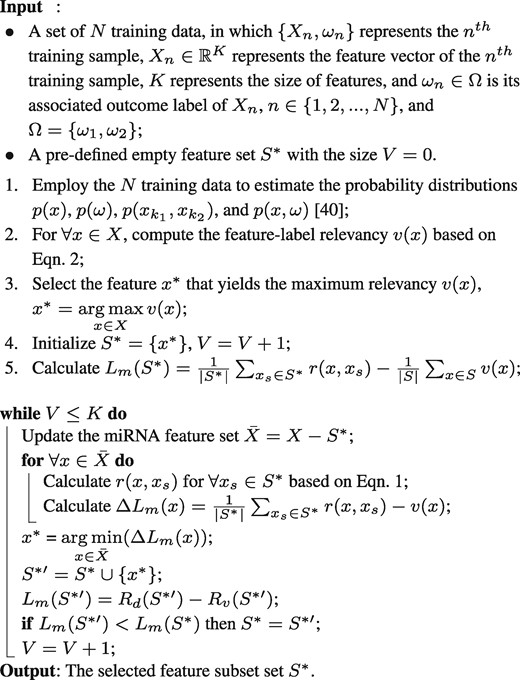
Given a training dataset, a subset yielding high feature-label relevance and low feature-feature redundancy is determined by minimizing in Equation 3 with an incremental searching strategy shown in Algorithm 1.
2.3 BFT-based miRNA biomarker refinement
The goal of feature refinement is to further select a feature subset from the determined by mRMR method described above. This refinement process relates to the performance of a classifier. The feature refinement process was designed based on BFT theory (Dempster, 2008; Shafer, 1976; Wu et al., 2019), considering its ability of reasoning with uncertain and imprecise information by aggregating partial and uncertain evidences. BFT is a generalization of both probability theory and set-membership approaches, and closely relates to imprecise probability (Walley, 2000) and random sets (Nguyen, 2006). The traditional Bayesian classification considers the probability of a sample’s label belonging to each class, but BFT-based feature refinement method considers not only the probability of a sample belonging to each single label but also belonging to the subsets of all labels, which can deal with class label imprecision and uncertainty (the challenges described in this study).
In this study, four possibilities of a sample’s class label were considered and defined as , in which represents an empty label set. In this way, the uncertainty of a sample’ label is handled more precisely than only separating the possibilities of a sample’s label belonging to either ω1 or ω2. Let ω denote the label of a sample X, the evidence regarding the actual value of ω can be represented by a mass function m on Ω, which was defined from the power set to the interval :
where m(A) denotes a degree of belief attached to the hypothesis that . The mass function induced by a sample Xi, which supports the assumption that another sample Xj has the same class label of Xi, is defined as:
where , α and γc are the weight factors, and represents the distance between Xi and Xj:
where represents the Euclidean distance between the vth feature of Xi and that of Xj, , and λv represents an element in Λ. Large represents negligible information provided by the vth feature of Xi to Xj. Given a set of N samples Xn, , which can be separated into two groups of samples, and , with different labels ω1 and ω2, respectively. The mass function induced by the set of N samples, which supports the assumption that the sample Xi has the same class label of , is defined as:
Algorithm 1: mRMR-based miRNA feature pre-selection strategy
where when Θc is empty. A global mass function Mi regarding the class membership of Xi can be calculated as:
Defining a binary vector Λ with the size of the number of elements in , the goal of feature refinement process is to determine the value of an element λ in Λ to be either 0 or 1. In the determined Λ, 1 represents the corresponding feature in was selected, while 0 represents the feature was not selected. The refined feature subset is those features corresponding to λ = 1. Given the definition of mass function and global mass function, each λ in Λ can be determined through the minimization of a loss function :
The first item in measures the mean squared error between the predicted probability scores and the outcome labels in the feature subspace determined by Λ. Here was defined as:
where represented a global mass function that quantifies the level of evidence that sample Xn has class label of ωc, and when the label of Xn was ω1, and , and when the label of Xn was ω2.
The second item in was defined as:
where defined in Equation (10) measures the conflict in the neighborhood of Xn, and measures the imprecision regarding the class membership of Xn (Wu et al., 2019). The item and item work together to select the features which can correctly estimate samples’ labels and penalize a feature subset that results in conflict and imprecise evidence. The features are selected by considering both the uncertainties of features and class labels and other issues through the training process.
Last term is a sparsity constraint, in which represents the number of non-zero entries in Λ and β is a scalar that controls the strength of the sparsity penalty. This term forces the selected miRNA feature subset to be sparse in order to decrease the over-fitting risk on unseen data, and lead to high classification accuracy and small overlaps between different classes.
2.4 EK-NN classifier for patient stratification
The EK-NN classifier (Denoeux, 1995; Denœux and Kanjanatarakul, 2016; Lian et al., 2016a; Liu et al., 2017; 2018) was employed as the pre-defined classifier for the feature refinement and the final classifier for stratifying unseen data as well. The original voting K-NN (Dudani, 1976) assigns a sample into the class represented by its majority nearest neighbors in the training set without concerning the dissimilarity (distance) between the sample and its neighbors. To endow the K-NN method with the capability to consider the sample dissimilarity to better handle the uncertain information, the EK-NN rule provides a global treatment of partial knowledge regarding the class membership of training patterns. Ambiguity and distance reject options are also taken into account based on the concepts of lower and upper expected losses (Quost et al., 2011). The EK-NN method has outperformed other traditional K-NN methods in many situations when using the same information (Zouhal and Denoeux, 1998).
The parameters α and γc in Equation (7) were determined along with the minimization of the loss function defined in Equation (11). The loss function was minimized by use of an integer genetic algorithm (Damousis et al., 2004). The determined parameters α and γc were then employed to calculate the mess-functions in Equation (7) which were employed to measure the differences (mass-function based distances) of a given sample to its neighbors and stratify it. In addition, to overcome the challenge of feature selection with imbalance data, an adaptive synthetic sampling (ADASYN) (He and Garcia, 2008) was employed to rebalance data by generating synthetic minority class samples according to their distribution. The key idea of ADASYN is to create synthetic samples according to the distribution of the minority class samples, where more samples are generated for the minority class samples that have higher difficulty in learning. The level of difficulty in learning for each minority samples is measured by the ratio of the majority class samples in each minor class sample’s k-nearest-neighborhood. In this study, five neighbors are considered for the minor class data re-balance according to the processed data. ADASYN outputs a balanced training dataset via the procedure described in the literature (He and Garcia, 2008; Lian et al., 2015).
2.5 Prognosis model training and validation
In this study, overall survival (OS) and disease-specific survival (DSS) were employed as the end points of treatment outcome, respectively. The proposed method was trained and tested separately to stratify low-risk and high-risk patients based on either OS or DSS. Of all 150 samples, 101 samples were randomly selected as the training set while the rest 49 samples were considered as the testing set based on OS labels. The training dataset included 40 OS positive and 61 negative cases, and the testing dataset included 11 positive and 38 negative cases, respectively. Positive cases represent survival and negative represents not. The same separation strategy was also employed to determine training and testing datasets based on the DSS label, of which 41 positive and 60 negative cases were included in the training datasets and 13 positive and 36 negative cases were included in the testing datasets. Five-fold cross validation was employed to train and validate the proposed method. The training data was used alone without involving any testing data. The hyperparameters, α, β and the number of neigbors in EK-NN, were optimized individually through the line search. The model that achieved the lowest validation loss, which is the average loss over the folds, was employed for the final evaluation on the testing data. In addition, the searching range of the parameters was summarized in Table 1. The range is determined considering that (i) β should be much less than 1 for reasonable sparsity of features, (iii) α should be close to 1 considering small uncertainty of features and labels and (iii) the numbers of neighbors is chosen from the commonly setting of that in K-NN methods.
The parameters to be determined through the training process
| Parameters | Range of settings |
|---|---|
| β in Equation 11 | determined from |
| No. of the neighbors in EK-NN | determined from |
| α | determined from |
| γc | = and determined through loss function minimization, |
| where represents the mean distance | |
| between any two samples with the same ωc |
The prediction accuracy, F1 score, the area under the receiver operating characteristic curve (AUC), and Kalpan Meier survival curves (Bland and Altman, 1998) were employed to evaluate the performance of the proposed method. The prediction accuracy is defined as: , and the F1 score is defined as: . Here Tp is the number of positive cases that are correctly predicted as positive ones, Tn is the number of negative cases that are correctly predicted as negative ones, Fp is the number of the cases that are predicted to be positive but in fact are negative ones, and Fn is the number of the cases that are predicted to be negative but in fact are positive ones. The F1 score is an effective metric for evaluating prediction performance when having imbalanced testing dataset. The ROC curve and the area under the ROC curve (AUC) were also employed to visualize the stratification performance. The AUC was calculated based on the ROC curves fitted by use of the tools developed by Metz (1999). The Kaplan Meier curves were plotted by use of Kaplan–Meier analysis methods (Bland and Altman, 1998) and the open-source software (Creed et al., 2020).
3 Results
Figure 2 showed the performance of the proposed method on stratifying patient cases based on OS and DSS as the endpoints of the outcome, respectively. It can be observed that the proposed method achieved high performance. The proposed model has been further evaluated through the comparison with other state-of-the-arts methods. The results were shown in Figures 3 and 4. The first compared method is the cox proportional hazards regression (CoxReg) analyses-based method (Cox, 1972; Gao et al., 2013), which is one of the most popular regression techniques for survival analysis. The BFT-based evidential forward feature selection (EFS-BFT) method (Lian et al., 2015), and the RELIEF-based BFT (RELIEF-BFT) method (Lian et al., 2015) were also compared to the proposed mRMR-BFT method. In the EFS-BFT method, a BFT-based feature selection method was directly applied to all profiled miRNA features to select a sparse subset. In the RELIEF-BFT method, the RELIEF algorithm (Kira and Rendell, 1992b) was employed to pre-select informative features based on feature-label relevance, and then BFT-based feature refinement was applied to determine the final sparse subset of miRNA features. In the mRMR-BFT method, the feature set selected by the mRMR method was refined to a sparse feature set by use of the BFT method. The EK-NN classifier was employed as the pre-defined classifier to train all these compared methods excluding the CoxReg method. The EK-NN classifier, which was trained by use of all profiled features directly, was also compared to demonstrate the significance of feature selection process. The same training and testing data separation were employed for other compared methods for fair comparison. The parameters in all methods were optimized separately to achieve the best performance of each. The comparison results show that the proposed mRMR-BFT method achieved higher performance in terms of the metrics of prediction accuracy, AUC and F1 score.
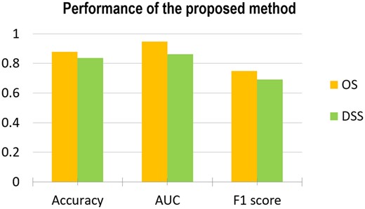
Performance of the proposed method evaluated by use the matrices of Accuracy, AUC and F1 score and based on the outcome labels of OS (a) and DSS (b), respectively
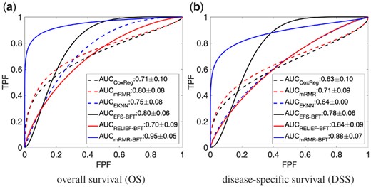
Performance comparison of the proposed method and five other methods. The performance was evaluated by use of ROC curves and AUC values and considering the overall survival OS (a) and disease-specific survival DSS (b) as the outcome labels, respectively
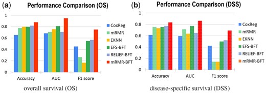
Performance comparison of the proposed method and five other methods. The performance was evaluated by use of the matrices of Accuracy, AUC and F1 score and based on the outcome labels of OS (a) and DSS (b), respectively
The effectiveness of the minor class data re-balance has been evaluated. Figure 5 showed the performance of the proposed method with and without data imbalance. In addition, the effectiveness of minor data re-balance was evaluated with the K-NN classifier. The results showed that minor class data re-balance improved the classifier performance on patient stratification. The effectiveness of the feature pre-selection process to improve the stratification performance of the learned EK-NN classifier was investigated. Figure 6 showed the prediction performance of the learned EK-NN prediction model by use the proposed mRMR-based method and four other pre-selection methods. These compared methods, which are independent to the classification performance, include RELIEF (Kira and Rendell, 1992a), mutual information maximization (MIM) (Fano and Hawkins, 1961) and mutual information feature selection (MIFS) (Battiti, 1994), and the random-forest method (Lin and Jeon, 2006). For fair comparison, a BFT-based feature refinement method was employed to refine the features pre-selected by these three methods, and the EK-NN-based classifier was employed as the pre-defined classifier for outcome prediction. The BFT method was directly applied to all profiled miRNA features to select a sparse subset to demonstrate the performance without any feature pre-selection. The parameters in all methods were optimized to achieve the best performance of each. The proposed mRMR-BFT method showed superior performance by selecting features considering both high feature-label relevance and low feature-feature redundancy.
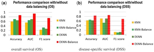
Comparison of the proposed method with and without minor-class data balance. The classical K-NN method with and without data balance were compared as well
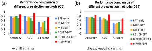
Comparison of the mRMR-based feature pre-selection and other four feature pre-selection methods. The selected features from the five methods were employed to refine the features and the EK-NN classifier. BFT-only feature selection method was also compared. The performance was measured by use of the metrics of Accuracy, AUC and F1 score and based on the outcome labels of OS (a) and DSS (b), respectively
The BFT-based feature refinement method was compared with other two widely used feature methods, the genetic algorithm (GA) (Davis, 1991) and the binary particle swarm optimization (BPSO) (Kennedy and Eberhart, 1997) methods. Both GA and BPSO methods require a pre-defined classifier for feature selection. Here, the mRMR-based selection method was uniformly employed as the feature pre-selection method for fair comparison. As shown in Figure 7, the proposed mRMR-BFT based method achieves superior prediction performance in terms of Accuracy, AUC and F1 score, compared to the other two methods.
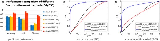
Comparison of the BFT-based feature refinement method and two other feature refinement methods. The features selected by mRMR methods were employed as the input of three methods (a). The performance measured by use of metrics of Accuracy, AUC and F1 score (a). The ROC curves and corresponding AUC values by use of OS (b) and DSS (c) as the outcome labels
The 5-year Kaplan–Meier survival curves were plotted for the prediction results of the proposed mRMR-BFT method and the other five compared methods (CoxReg, EFS-BFT, RELIEF-BFT, MIM-BFT and MIFS-BFT). The patients in the testing cohort were stratified into either the high-risk group or low-risk group based on the same threshold risk score determined by the training cohort of each of the compared methods. As shown in Figures 8 and 9, the proposed mRMR-BFT method can stratify high-risk and low-risk patient groups more accurately compared to the other five methods.
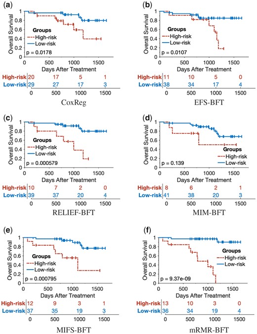
Kaplan–Meier survival analysis to evaluate the performance of the proposed method and other five compared methods by use of OS as outcome labels
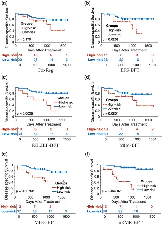
Kaplan–Meier survival analysis to evaluate the performance of the proposed method and other five compared methods by use of DSS as outcome labels
Table 2 shows the selected informative miRNA features by use of the proposed method and the other four methods: CoxReg, EFS-BFT, RELIEF-BFT and mRMR-only. In the CoxReg method (Gao et al., 2013), a subset of 6 miRNA features were selected by use of multi-variate cox regression, which were employed to learn a cox regression model for stratifying patients into high-risk and low-risk groups. In the mRMR method, 13 miRNA features were selected and employed to train the EK-NN classifier directly without performing feature-refinement. A total of 5 and 8 features were selected by the EFT-BFT and RELIEF-BFT methods, respectively. In the proposed mRMR-BFT method, 13 miRNAs were pre-selected by the mRMR method, and then were refined to 6 features by use of the BFT-based refinement process through the optimization of the EK-NN classifier. It showed that less features were selected and the feature sparsity is high.
The miRNAs selected by varied methods
| Methods | Selected miRNAs |
|---|---|
| CoxReg | miR-24, miR-31, miR-193b, miR-26b, miR-142-3p, miR-146a |
| mRMR-only | miR-31, miR-24, miR-215, miR-103, miR-26b, miR-25, miR-7, miR-148a, miR-30a-5p, miR-130a, miR-191, miR-16, miR-128b |
| EFS-BFT | miR-7, miR-9, miR-99a, miR-210, miR-220 |
| RELIEF-BFT | miR-24, miR-31, miR-34c, miR-92, miR-135b, miR-210, miR-215, miR-328 |
| mRMR-BFT | miR-7, miR-25, miR-31, miR-130a, miR-191, miR-215 |
4 Discussion
In this study, a novel and systematic machine learning-based strategy was proposed to reliably stratify subsets of OPSCC patients with low and high risks of treatment failure. The proposed strategy included a two-stage feature selection procedure and an EK-NN classifier to address the challenges described above in Section 1. The model can serve as a clinical decision-making tool to (i) readily identify the subset of patients with low risk that would benefit from de-intensifying treatment, and (ii) accurately identify high risk patients for whom de-intensification would be detrimental and who may require further intensification. The designed method has several innovations. First, by use of appropriate methods to address the challenges in each step of outcome prediction, the overall performance is improved which is demonstrated by the prediction results when compared with other methods. The mass functions considered the possibilities of a sample belong to each single label and the combinations of multiple classes and addressed the uncertainty of features and labels of samples. In addition, the model was designed with a modularized structure, which facilitates the change of any one or several modules for classification performance evaluation/comparison and facilitate the incorporation of other state-of-the-art modules. The modularized design can provide a seamless integration of each component.
Some future research directions can be summarized as below. First, the proposed method was to train a prediction model for predicting oropharygneal cancer treatment outcome and patient stratification. It forms a basis for biomarker and/or feature-based cancer treatment outcome prediction, and can be generalized to other type of cancer treatment outcome prediction scenarios. It was observed that the features selected (retained) from the total of 96 miRNA features show great variability in this study (Table 2). All these 96 miRNAs have been proved to be related to OPSCC outcomes. The selected feature subset relates to feature selection methods and classifiers. Further radiobiology investigation might be required to provide more information for future study. The proposed method should be further evaluated when larger clinical dataset is available. The performance improvement by using data-rebalancing process should be investigated with large datasets as well.
Second, radiomics, the high-throughput extraction and analysis of numerous features from medical images, is a highly promising approach for characterizing tumor phenotype, which provides an unprecedented opportunity to support and improve personalized clinical decision-making (Wu et al., 2019; Yip and Aerts, 2016) For several tumor sites, imaging biomarkers have shown promise in accurately separating favorable and unfavorable prognosis patients. Clinic features, such as gender, age and tumor stage, may also convey useful information for outcome prediction. However, current efforts to utilize high-dimensional multimodal biomarkers for early disease prognosis and treatment outcome prediction have also been compromised due to the above-mentioned challenges. Designing multimodal biomarker-based prognosis model can be potentially useful to learn a powerful and robust model for predicting treatment outcomes of oropharyngeal cancer and other cancer types. The thoughtful investigation of the correlation, independence and complementary nature of multimodal biomarkers (imaging, genomics, clinical and histopathologic biomarkers) remains unexplored, and requires further studies.
Third, deep learning methods have been applied in various fields and showed promising results. However, supervised deep learning methods have not been employed in this study, mainly because that the number of training samples is too small to well train a deep neural network, and data from single-modal has been employed, which will severely decrease the generalization ability of deep learning method. To study how to process multimodal data with deep learning method is a challenging task but an interesting research work that might provide more robust patient stratification and outcome prognosis. In addition, it will be interesting to assess the informativeness of the features extracted by use of deep learning methods and compare their performance with that of the features selected by traditional machine-learning methods.
5 Conclusion
A novel and systematic machine learning-based strategy was proposed to learn a prediction model with miRNA features for the stratification of oropharyngeal cancer patients with low and high risks of treatment failure. The prognosis model can be employed as a supporting tool to identify patients who are likely to fail standard therapy and potentially benefit from alternative or targeted treatments.
Funding
This work was supported by National Institutes of Health Award [R01DE026471, R01CA233873 and R21CA223799].
Conflict of Interest: none declared.
References
Denœux T. (2008) A k-nearest neighbor classification rule based on Dempster-Shafer theory. In: Yager R.R. and Liu L. (eds) Classic Works of the Dempster-Shafer Theory of Belief Functions. Studies in Fuzziness and Soft Computing. Vol 219. Springer, Berlin, Heidelberg. 10.1007/978-3-540-44792-4_29.

