Protein contact map refinement for improving structure prediction using generative adversarial networks

Abstract

Motivation

Protein structure prediction remains as one of the most important problems in computational biology and biophysics. In the past few years, protein residue–residue contact prediction has undergone substantial improvement, which has made it a critical driving force for successful protein structure prediction. Boosting the accuracy of contact predictions has, therefore, become the forefront of protein structure prediction.

Results

We show a novel contact map refinement method, ContactGAN, which uses Generative Adversarial Networks (GAN). ContactGAN was able to make a significant improvement over predictions made by recent contact prediction methods when tested on three datasets including protein structure modeling targets in CASP13 and CASP14. We show improvement of precision in contact prediction, which translated into improvement in the accuracy of protein tertiary structure models. On the other hand, observed improvement over trRosetta was relatively small, reasons for which are discussed. ContactGAN will be a valuable addition in the structure prediction pipeline to achieve an extra gain in contact prediction accuracy.

Availability and implementation

https://github.com/kiharalab/ContactGAN.

Supplementary information

Supplementary data are available at Bioinformatics online.

1 Introduction

Protein structure prediction remains as one of the most important problems in biology, more specifically in bioinformatics, biophysics and structural biology. Tremendous efforts have been paid for determining tertiary structures of proteins because the structures provide indispensable information for understanding the principle of how proteins carry out biological functions, developing drug molecules and artificial protein design. To supplement experimental methods of structure determination, computational protein structure prediction methods have been developed over the last three decades.

As observed in the community-wide protein structure prediction experiments, the Critical Assessment of techniques in protein Structure Prediction (CASP) (Kryshtafovych et al., 2019) the accuracy of prediction methods has significantly improved in the past few years. The main driver behind this accuracy boost is the improvement of residue–residue contact or distance prediction, which is used effectively to guide the construction of protein structure models. Residue contacts or distances of a protein are predicted from a multiple sequence alignment (MSA) of the protein. Predicting residue contacts from an MSA has over 20 years of effort by different research groups toward establishing accurate prediction methods. In principle, evolutionary constraints for maintaining residue–residue contacts in a protein structure leave a trace in the MSA of the protein of interest and its homologous proteins. Earlier works applied relatively simple statistical approaches to an MSA (Fariselli et al., 2001; Ortiz et al., 1998). The accuracy of contact prediction was substantially improved a few years ago when the so-called co-evolution approaches, which use statistical inference based on the Potts model (Ekeberg et al., 2013), were introduced. The methods in this category include CCMpred (Seemayer et al., 2014), Gremlin (Kamisetty et al., 2013), EVFold (Marks et al., 2011), plmDCA (Ekeberg et al., 2013), FreeContact (Jones et al., 2015; Kaján et al., 2014) and MetaPSICOV (Jones et al., 2015). Further improvement was observed more recently when deep learning, Convolutional Neural Networks (CNN) and Residual Networks (He et al., 2016), were applied to the problem. The methods in this category include DeepCov (Jones and Kandathil, 2018), RaptorX-contact (Wang et al., 2017), DeepContact (Liu et al., 2018) and trRosetta (Yang et al., 2020).

Although substantial improvement in contact prediction has been observed, contact prediction is still far from perfect. Here, we propose ContactGAN, a novel contact map denoising and refinement method using Generative Adversarial Networks (GAN) (Goodfellow et al., 2014). GANs have been widely adopted for high-level generation tasks in computer vision with applications including image-to-image translation (Zhu et al., 2017), and image super resolution (Ledig et al., 2017). ContactGAN takes a contact map predicted by existing methods, which is considered as an imperfect, noisy input and outputs an improved map that better captures correct residue–residue contacts compared to the original map. ContactGAN was trained with predicted noisy contact maps coupled with corresponding native contact maps, which the networks were guided to generate. We show that we gain a consistent and substantial precision improvement over predicted maps by CCMpred, DeepCov and DeepContact, on the validation dataset, the CASP13 and the CASP14 datasets. It was also demonstrated that combining multiple predicted maps computed by different methods further improves the accuracy of generated maps. On the other hand, the improvement over trRosetta was relatively small. The potential reasons for that are extensively discussed. ContactGAN can be the powerful last step of a contact prediction pipeline to improve any existing contact prediction methods as demonstrated through application to the four contact prediction methods.

2 Materials and methods

2.1 Protein structure and contact map dataset

We prepared a dataset of 5263 non-redundant protein structures, for each of which a contact map was computed by four existing contact map prediction methods. The predicted contact maps, together with the native (i.e. correct) contact maps, were used for training ContactGAN. A native contact map we use contains binary values, 1 or 0, where 1 indicates that the Cβ atom distance of the corresponding residue pair is 8 Å or shorter.

The protein dataset was constructed based on the PISCES (Wang and Dunbrack, 2005) protein dataset selected with a 25% sequence identity, which was released before May 2018 (i.e. the beginning of CASP13). All these proteins were solved by X-ray or Nuclear Magnetic Resonance. From the PISCES dataset, proteins longer than 700 amino acid residues or shorter than 25 amino acid residues were discarded. Proteins were also excluded if they contain unknown amino acids in their sequence, have a knot in the structure that was checked by referring to the KnotProt2.0 database (Dabrowski-Tumanski et al., 2019), or have consecutive missing residues up to two residues in the structure. Structure gaps up to two residues were filled with the Modeller (Eswar et al., 2006) automodel protocol. This step yielded 6640 protein structures. To further ensure non-redundancy of structures, we filtered the remaining proteins based on the CATH structural classification database (Knudsen and Wiuf, 2010). We first removed proteins that are not in the latest CATH-domain list and proteins in Class 6 (special structures), which yielded 5263 proteins. We then split these proteins into training and validation datasets such that there were no overlapping CATH codes up to the topology (T) level. The split was also made to ensure that both datasets have sufficient presence of all 4 CATH classes. The final counts of proteins in the training and validation datasets were 4962 and 301, respectively.

In addition to this dataset, we used all the 43 contact prediction (RR) target domains in CASP13 and all the 49 RR targets in CASP14 as independent test sets. They are listed in Supplementary Table S1.

2.2 Predicting contact maps with four existing methods

We used four existing prediction methods, CCMpred, DeepContact, DeepCov and trRosetta, to predict contact maps of the proteins in the dataset described above. Input MSAs were generated using DeepMSA (Zhang et al., 2020). We used HHsuite (Steinegger et al., 2019) version 3.2.0 and HMMER (Potter et al., 2018) version 3.3 in DeepMSA. For sequence databases, Uniclust30 database (Mirdita et al., 2017) dated October 2017, Uniref90 (Suzek et al., 2015) dated April 2018 and Metaclust_NR database (Steinegger and Söding, 2018) dated January 2018 were used. These database releases are before CASP13 has started.

CCMpred is a baseline contact prediction method, which uses the Pseudo-Likelihood Maximization of direct couplings between pairs of amino acids in an MSA of the target protein (Seemayer et al., 2014). DeepContact is one of the deep learning-based contact prediction methods (Liu et al., 2018). We used the DeepContact code made available at Github by the authors. DeepCov is another method that uses deep learning (Jones and Kandathil, 2018). trRosetta uses the ResNet CNN architecture (He et al., 2016). It was shown that trRosetta had superior performance to other existing methods on the CASP13 dataset. For trRosetta, we generated MSAs at three different E-values in the HHblits search steps of the DeepMSA pipeline, 0.001, 0.1 and 1.0. Since trRosetta outputs predicted distance between residue pairs, we used a distance cutoff of 8 Å to decide if two residues are in contact. Since we ran trRosetta with three MSAs of different E-value cutoffs, we obtained three different contact predictions, which were considered as a 3-channel input for ContactGAN.

2.3 Architecture of ContactGAN

ContactGAN takes a predicted contact map by four prediction methods mentioned above as input and outputs a refined map. ContactGAN adopts the GAN framework, where two networks, a generative and a discriminative network, are trained with sets of predicted (noisy) and corresponding native (i.e. correct) contact maps so that refined maps can be generated by learning patterns from predicted and native maps. A native contact map we use contains binary values, 1 or 0, where 1 indicates that the Cβ atom distance of the corresponding residue pair is 8 Å or shorter.

Figure 1 shows the network structure of ContactGAN. Figure 1a illustrates the overall architecture. The generator network, illustrated in Figure1b, is a CNN consisting of a 2D convolution layer with 32 channels and a kernel size of 9, which is followed by 9 or 18 ResNet blocks, a 2D convolution layer and finally by a sigmoid layer. 18 ResNet blocks were used when refining contact maps generated by trRosetta and 9 for all the other methods. The discriminator network (Fig. 1c) is a fully convolutional binary classifier. It takes a contact map output from the generator and the corresponding native contact map and classifies the two maps into classes, either native (correct) or predicted. The discriminator network consists of 4 units of the combined ‘Conv2d+IN’ block (pink) and ‘Conv2d+IN+Dropout’ followed by one unit of Conv2d+IN with 512 channels, conv2d with 512 channels and a sigmoid layer. The details of these blocks are shown in Supplementary Figure S1.

Fig. 1.

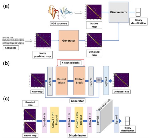
The architecture of ContactGAN. (a) The overall structure that connects the generator and the discriminator networks. (b) The network structure of the generator network. X is equal to 18 for handling maps from trRosetta and 9 for the other methods. (c) The detailed structure of the discriminator network. See text for more details

2.4 Parameter training for ContactGAN

A contact map predicted by a contact map prediction method (e.g. CCMpred), which we hereby refer to as a noisy map, is an input to the generator network of ContactGAN. The output map of the generator network and the corresponding native contact map of the noisy map were then used as inputs to the discriminator network. Out of 5263 pairs of noisy and native contact maps, 4962 pairs were used for training and 301 were used for validation. ContactGAN was trained separately for each contact prediction method using predicted maps and corresponding native contact maps. Note that protein sequence information and other features, such as MSA and secondary structure prediction, were not used in ContactGAN.

For training GANs, the generator and discriminator networks are trained together with a min-max game-style objective function given by Equation (1):

$$\underset{G\mathrm{ }}{\min \mathrm{ }}\underset{D}{\max }\begin{array}{c}E\\ x \sim {\mathbb{ }\mathbb{P}}_d\end{array}\left[\log D\left(x\right)\right]\mathrm{ }+\mathrm{ }\begin{array}{c}E\\ z \sim {\mathbb{P}}_g\end{array}\left[\log \mathrm{ }(1-D(z)\right)]\mathrm{ }$$

(1)

where G and D are parameters of the generator and the discriminator networks of ContactGAN, ${\mathbb{ }\mathbb{P}}_d$ is the real (correct) data distribution, ${\mathbb{P}}_g$ is the generated (fake) data distribution, D(x) and D(z) are predicted probabilities by the discriminator that the real (x) and fake data z are real. The generator receives noisy data as input and generates denoised data. The discriminator then classifies input data to denoised data or real data. The minimax objective ensures that the generator generates good quality denoised data that can fool the discriminator into classifying denoised data as real data. Following the above common practice for general GAN, the objective function for ContactGAN is formulated as shown in Equation 2, which is a linear combination of a content loss and an adversarial loss:

$$\mathit{Loss}={\mathit{Loss}}_{\mathit{content}\mathrm{ }}+\mathrm{ }{10}^{-3}\mathrm{ }{\mathit{Loss}}_{\mathit{adversarial}\mathrm{ }},\mathrm{ }$$

(2)

where$\mathrm{ }$  

$${\mathit{Loss}}_{\mathit{content}\mathrm{ }}=\mathrm{ }\sum _{i=0}^L\sum _{j=0}^L{\left(T_{i,j}-{\left(G\left(N\right)\right)}_{i,j}\right)}^2\mathrm{ }$$

(3)

 

$${\mathrm{and}\mathrm{ }\mathit{Loss}}_{\mathit{adversarial}\mathrm{ }}=\mathrm{ }-D\left(G\left(N\right)\right)\mathrm{ }$$

(4)

Here, L is the protein sequence length, T corresponds to the native contact matrix (map), and N is the input predicted (noisy) contact matrix, G(N) is the denoised matrix and D(G(N)) is the discriminator’s prediction of the denoised map, which ranges between 0 to 1. We optimize the negative of D(G(N)), as we want to fool the discriminator to consider that the denoised map to be as good as the native map. The content loss is defined by the Mean Squared Error (MSE) between the denoised map and the native map. The adversarial loss is given as the negative softmax probabilities of the discriminator predictions.

We employed the Two Time-scale Update Rule (TTUR) (Heusel et al., 2017) to use separate learning rates for the generator and the discriminator for stable GAN training. We used learning rates of 0.0001 for the generator and 0.0004 for the discriminator (Supplementary Note S1). The batch size was set to 1 as contact maps (i.e. proteins in the dataset) are of different sizes. ContactGAN was trained for 50 epochs (Supplementary Fig. S2). We choose the best performing model on the validation dataset for testing the CASP13 and CASP14 test datasets. The computational time needed for training and inference is provided in Supplementary Table S2.

2.5 Building structure models from a contact map

To build protein structure models from the predicted contact map, we used the energy minimization protocol, MinMover, in pyRosetta (Chaudhury et al., 2010). Detailed procedure is explained in Supplementary Note S2.

3 Results

ContactGAN was evaluated on three datasets, the validation set in the non-redundant protein dataset as well as the CASP13 and CASP14 contact prediction targets. We evaluated whether ContactGAN could improve the quality of predicted contact maps by the four existing methods, CCMpred, DeepContact, DeepCov and trRosetta.

3.1 Contact map improvement with ContactGAN

In Table 1, we summarize ContactGAN’s performance in improving residue contact map prediction on the validation set and the CASP13 set. In this table, we only showed precision considering predicted contacts with the top L/1 highest probabilities (L is the length of the protein). Results with more metrics are provided in Supplementary Tables S3–S5. Supplementary Figure S3 shows improvements of the precision of individual predicted contact maps on the validation and the CASP13 datasets.

Table 1.

Improvement on L/1 prediction by ContactGAN

Method	Validationa		CASP13
	Med+Lgb	Lg	Med+Lg	Lg
CCMpred	0.245	0.193	0.164	0.121
	0.421	0.333	0.287	0.217
DeepCov	0.457	0.349	0.320	0.231
	0.470	0.361	0.368	0.250
DeepContact	0.450	0.351	0.382	0.267
	0.480	0.374	0.408	0.283
C + Dvc	0.457	0.349	0.320	0.231
	0.523	0.410	0.402	0.284
C + Dt	0.450	0.351	0.382	0.267
	0.514	0.405	0.420	0.299
Dv + Dt	0.450	0.351	0.382	0.267
	0.521	0.411	0.438	0.310
C + Dv + Dt	0.450	0.351	0.382	0.267
	0.537	0.426	0.437	0.314
trRosetta	0.702	0.583	0.657	0.510
	0.707	0.585	0.667	0.516
9 blocksd	0.696	0.580	0.650	0.512

Note: Results shown are for top L/1 prediction.

a

Results of two datasets are shown: On the left, the validation set of 301 proteins in the non-redundant protein dataset; on the right, the CASP13 dataset.

b

The columns Lg consider only long-range contacts (residue pairs separated by more than 23 residues) while Med+Lg columns consider medium- and long-range contacts (residue pairs separated by more than 11 residues).

c

Each result corresponds to top L/1 contact predictions with the highest probabilities where L is the length of the protein. Two values shown: up, original average precision by the existing method; bottom, average precision of denoised contact maps by ContactGAN. In the middle rows, contact maps of two or three methods were used as input: C, CCMpred; Dv, DeepCov; Dt, DeepContact. When multiple maps were used as input, the highest precision among the existing methods was shown as the original results. For trRosetta, three independent contact predictions were combined, each of which used an MSA with different E-value cutoffs, 0.001, 0.1 and 1.0.

d

Nine blocks of ResNet were used in the generator.

The first three rows in Table 1 show results for individual methods, CCMpred, DeepCov and DeepContact. ContactGAN made substantial improvements for these methods in all the metrics, which was consistent between the validation set and the CASP13 set. Particularly, the improvements were largest for CCMpred, which had the lowest original precision among the three methods. For CCMpred, ContactGAN improved L/1 Long precision on the validation set from 0.193 to 0.333, an improvement of 72.5%. For the CASP13 set, the improvement for L/1 Long was slightly larger, 79.3% (from 0.121 to 0.217). The improvement ranged from 71.8% to 79.3% for other metrics shown in Table 1 for CCMpred. The improvement was also consistent for DeepCov and DeepContact, but with smaller improvement margins than observed for CCMpred. For DeepCov, ContactGAN showed an improvement of 3.43% and 8.23% for L/1 Long on the validation and the CASP13 sets, respectively. The corresponding values for DeepContact were 6.55% and 5.99%, respectively.

The middle rows in Table 1 present ContactGAN performance using multiple channels, where a pairwise combination of the above three methods and all three methods together were used as input channels. To be able to take two or three contact maps as input, the network architecture of ContactGAN was modified accordingly. The row with ‘C + Dv’ shows the precision values with CCMpred and DeepCov as two input channels for ContactGAN. With these two channels, ContactGAN showed substantial improvement in every evaluation category over the two individual methods. It is interesting to note that the improvement was achieved not only over CCMpred, the method with lower accuracy, but also over the better method, DeepCov. We see similar improvements when CCMpred+DeepContact and DeepCov+DeepContact were used as two-channel inputs. Then, we further extended the use of multi-channels to three channel inputs with CCMpred, DeepCov and DeepContact altogether (C+Dv+Dt in the table), which resulted in a further improvement over two channel inputs.

Improvements by combining additional method(s) are apparent in Figure 2, where L/1 Long precision values of each individual method and its combinations with other methods are compared. From originally predicted contact maps predicted by a single method, ContactGAN improved them with a large margin, which was further improved by using additional contact maps predicted by different methods (2 input channels). Furthermore, an even higher precision was achieved by using three methods as input.

Fig. 2.

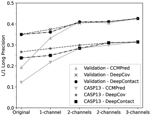
Improvement of L/1 Long precision by using additional predicted contact maps as input channels. Two sets of lines are shown for validation and CASP13 results for each of CCMpred (solid gray line), DeepCov (dashed line) and DeepContact (dashed and dotted line). Original indicates precision of the original contact maps, X-channel(s) indicates predictions by GAN with X = 1,2 and 3 channels as inputs. In the case of 2 channels, every method has 2 possible combinations of input. The order of the combinations was as follows: For C: C+Dv, C+Dt. For Dv: C+Dv, Dv+Dt. For Dt: C+Dt, Dv+Dt. Precision values plotted are taken from Table 1

In the last row of Table 1, we show the results of the application of ContactGAN to trRosetta, a relatively new method which showed one of the best performances among those published and available (Yang et al., 2020). Since the base accuracy of trRosetta is significantly better than the other methods, we combined three different channels of trRosetta, each using different MSAs generated with a sequence E-value cutoff of 0.001, 0.1 and 1.0, respectively, instead of combining with the other methods. Compared with the best prediction among the results with the three E-values, which is 0.001, ContactGAN made small but consistent improvements for all the metrics. For L/1 Long, ContactGAN improved by 0.34% and 1.17%, for the validation set and the CASP13 set, respectively. The performance gains seen on trRosetta are lower than for the other methods, but these improvements in Table 1 have P-value <0.05 by t-test. Supplementary Table S5 provides P-values of other metrics. Supplementary Figure S3 shows change of the L/1 long precision values of individual contact maps.

The generator for trRosetta used a deeper network (18 ResNet blocks) than the networks for the other contact prediction methods (9 blocks) (Fig. 1). We also trained a generator with nine ResNet blocks for trRosetta and applied, which is shown in the last row of Table 1. The smaller generator showed a lower precision than the 18-block one, which was still better on average than the best among the original trRosetta (i.e. E-value of 0.001) for the CASP13 set (0.512). But for the validation set, the result (0.580) was worse than the best trRosetta with an E-value of 0.001. We further tested the performance of the network when only generator was trained without the discriminator. ContactGAN consistently showed better performance than the generator-only network (Supplementary Table S5).

We were also curious if a GAN trained on maps generated by one method was able to refine predicted maps by another method (Supplementary Fig. S4). As shown, overall ContactGAN could not improve maps if it was trained on maps by a different method, which implies that the trained GAN captured method-specific predicted contact patterns. One exception was observed when the GAN trained on DeepContact map was applied to DeepCov maps, where we see improvement on 22 maps out of 43 maps. Prediction accuracy of DeepCov and DeepContact are similar but the opposite case, i.e. GAN trained on DeepCov did not improve maps by DeepContact (Supplementary Fig. S4b).

Next, we investigated which types of contacts were improved by ContactGAN. Particularly, we examined contacts between residues in secondary structure elements, α-helix and α-helix (denoted as α − α below), β-strand and β-strand (β − β) and α-helix and β-strand (α − β). To quantify the change made by ContactGAN, we compared the fraction of correct contacts between secondary structure elements predicted among the top L/1 long-range contacts before and after applying ContactGAN (Supplementary Fig. S5). For both validation and the CASP13 set, all three types of correct secondary structure interactions increased. For the validation set, particularly the fraction of β − β correct contacts increased while correct α − α contact predictions were particularly increased in the CASP13 set consistently across different prediction methods. Thus, the secondary structure preferences observed in the validation set and the CASP13 set were not consistent.

3.2 CASP14 contact prediction dataset

We further tested ContactGAN on the 49 CASP14 contact prediction targets. Table 2 shows the L/5 and L/1 precisions and Supplementary Table S6 provides results on the full metrics. Similar to the results on the previous two datasets, consistent improvements were observed by ContactGAN. The margin of the improvements on the L/1 long precision was 1.58% (for DeepCov) to 57.0% (for CCMpred). The improvement for trRosetta was smaller, 2.45%, but the change of the distribution of L/1 long precision was statistically significant (P-value < 0.05). T-test results of other metrics are provided in Supplementary Table S6.

Table 2.

Improvement of L/1 precision on the CASP14 dataset

Method	CASP14
	L/5a		L/1
	Med+Lgb	Lg	Med+Lg	Lg
CCMpred	0.275	0.247	0.157	0.128
	0.379	0.314	0.255	0.201
DeepCov	0.496	0.417	0.322	0.253
	0.527	0.407	0.345	0.257
DeepContact	0.531	0.434	0.329	0.243
	0.551	0.445	0.352	0.252
C + Dvc	0.531	0.434	0.329	0.243
	0.571	0.483	0.377	0.275
C + Dt	0.496	0.417	0.322	0.253
	0.529	0.423	0.360	0.269
Dv + Dt	0.496	0.417	0.322	0.253
	0.581	0.477	0.381	0.292
C + Dv + Dt	0.496	0.417	0.322	0.253
	0.581	0.473	0.386	0.298
trRosetta	0.671	0.577	0.468	0.368
	0.671	0.591	0.474	0.377
9 blocks	0.667	0.580	0.461	0.365

a

Two results on CASP14 dataset are shown: On the left, top L/5 contact predictions with the highest probabilities; on the right, top L/1 with the highest probabilities. L is the length of the protein.

b

The columns Lg consider only long-range contacts (residue pairs separated by more than 23 residues) while Med+Lg columns consider medium- and long-range contacts (residue pairs separated by more than 11 residues).

c

Two values shown: up, original average precision by the existing method; bottom, average precision of denoised contact maps by ContactGAN. In the middle rows, contact maps of two or three methods were used as input: C, CCMpred; Dv, DeepCov; Dt, DeepContact. When multiple maps were used as input, the highest precision among the existing methods was shown as the original results. For trRosetta, three independent contact predictions were combined, each of which used an MSA with different E-value cutoffs, 0.001, 0.1 and 1.0.

3.3 Examples of improved contact map predictions

In this section, we show four examples of pairs of contact maps before and after applying ContactGAN. The first example (Fig. 3a) is a ContactGAN application to a map by CCMpred. For this large protein of 561 amino acids (PDB ID: 1HK8A), the original map by CCMpred is covered by noisy predictions with low probability values. In contrast, ContactGAN map denoised it into more distinct contact patterns, which yielded a 77.3% improvement in L/1 long-range precision from 0.357 to 0.633. The next example is the refinement on a DeepContact’s prediction (Fig. 3b). The right panel is from a two-channel ContactGAN with DeepContact and CCMpred as input. ContactGAN was able to clean the strong noise and improved the L/1 long precision from 0.396 to 0.622 over DeepContact. In Figure 3c, a map predicted by DeepCov for a 405 residue-long protein in the CASP13 dataset was improved by the three-channel ContactGAN. Similar to the previous two cases, the original map suffered from high noisy probability values for medium and long-range contacts, which were cleaned by ContactGAN. The last example was a refinement for a contact map by trRosetta (MSA E-value: 10⁻³) (Fig. 3d). Compared to the previous cases, the improvements by ContactGAN visually seem minor; however, they include enhancement of critical very long-range contacts between residues 12–18 and 112–118. These correct contacts were very weakly predicted by trRosetta with the min, max and the average values of 0.002, 0.143 and 0.03, respectively, which were strengthened to 0.003, 0.794 and 0.213, respectively. The precision improvement of L/1 long contacts was 14.5% overall. In Supplementary Figure S6, more examples of improved maps over trRosetta are provided where the improved margin was relatively large.

Fig. 3.

Examples of contact maps before and after applying ContactGAN. For each panel, the map on the left is the original one predicted by an existing method and the map on the right is the refined map by ContactGAN. The color scale shows predicted probability values of contacts, ranging from dark blue (0.0) to bright yellow (1.0). Contacts with the residue itself along the diagonal line are removed. (a) A contact map of Ribonucleotide-Triphosphate Reductase in E.coli [PDB ID: 1HK8A; 561 amino acids (aa)] predicted by CCMpred. The L/1 long precision improved from 0.357 to 0.633. (b) Mg-ATPase Nucleotide binding domain (PDB ID: 3GWIA, 164 aa). The two-channel ContactGAN with CCMpred and DeepContact improved L/1 long precision from 0.396 (by DeepContact) to 0.622. (c) A CASP13 target, enterococcal surface protein (CASP ID: T0987, PDB ID: 6ORI; 405aa). Three-channel ContactGAN improved over DeepCov. L/1 long precision of domain D1, before: 0.405; after: 0.589. For domain D2, before: 0.367; after: 0.536. (d) A CASP13 target protein. Filamentous haemagglutinin family protein (CASP ID: T0968s1, PDB ID: 6CP9; 126 aa). The original map was by trRosetta with E-value 0.001. L/1 long precision, before: 0.407; after: 0.466

3.4 Effect of contact map improvement in str. modeling

We further examined how the improvement in contact map prediction transfer to resulting protein structure models. Figure 4 shows GDT-TS (Zemla, 2003) of models built for the 35 CASP13 targets using predicted contact maps before and after applying refinement using ContactGAN. In Figure 4, we showed results of a one-channel, a two-channel, the three-channel ContactGAN and ContactGAN for trRosetta. The rest of the ContactGAN results are shown in Supplementary Figure S7. For each target, 180 models were generated using pyRosetta as described in Supplementary Note S2. Dependency of the modeling results on the probability cutoff of contact prediction and the folding protocols used are provided in Supplementary Table S7. The left column in Figure 4 shows the largest GDT-TS among the generated models while in the right column, the best energy models by the Rosetta score were considered. The improvements of the GDT-TS distribution by ContactGAN in all the panels are statistically significant (P-value < 0.05).

Fig. 4.

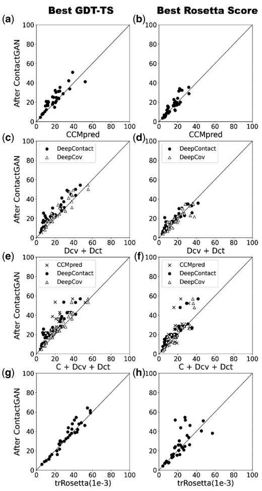
GDT-TS score of protein structure models generated with contact maps before and after ContactGAN. GDT-TS of structure models using predicted contact maps for the 35 CASP13 targets are shown. Out of 180 models generated (see Supplementary Note S2) the best GDT-TS score is shown in first column and values of the model with the best Rosetta score (the contact constraint term was not included) is shown in second column. X-axis, models built with original predicted contact maps; y-axis, with maps after applying ContactGAN. (a) Using maps predicted by CCMpred. The best GDT-TS value among the pool was plotted for each target. The number of targets where GDT-TS improved/tie/worsened after ContactGAN is 29/0/6 (P-value < 0.0001), respectively. We show these three numbers in this format for the rest of the panels. The number in the bracket indicates the P-value of the significance test conducted. (b) Maps by CCMpred. GDT-TS of the best Rosetta score models was plotted. 20/0/15 (0.009). (c) The two-channel ContactGAN with DeepCov (Dcv) and DeepContac (Dct). Circles, comparison against Dct; triangles, against Dv. Against Dct: 35/0/0 (< 0.0001); against Dcv: 27/0/8 (< 0.0001). (d) The best Rosetta score models for the 2-channel with Dcv and Dct. Against Dct: 25/0/10 (0.003); against Dcv: 20/1/14 (0.348). (e) A three-channel with CCMpred, Dcv and Dct. Crosses, CCMpred; circles, Dct; triangles, Dcv. Against CCMpred: 34/1/0 (< 0.0001); against Dcv: 28/0/7 (0.000); against Dct: 34/0/1 (< 0.0001). (f) GDT-TS of the best scoring models are plotted for the three-channel ContactGAN. Against CCMpred: 29/0/6 (< 0.0001); against Dcv: 25/0/10 (0.002); against Dct: 30/1/4 (< 0.0001). (g) trRosetta with the three E-value cutoffs. compared to trRosetta with E-value 0.001 (which performed the best among the three cutoffs): 22/1/12 (0.023). (h) the channel for trRosetta. Against trRosetta (E-value: 0.001): 19/0/16 (0.049). Plots for the other contact prediction methods are provided in Supplementary Figure S7.

Using a refined contact map by ContactGAN produced a higher GDT-TS model for a majority of the targets (panel a, c, e, g). The actual counts of improvements are provided in figure captions. This is also true for trRosetta (panel g), where the improvement is observed for 22 targets and 1 tie. When models selected by the Rosetta energy (the right column of the figures) were considered, the margin between the number of improved and worsened targets by ContactGAN shrank, but this is a scoring problem where the Rosetta energy failed to select better quality models. Model selection would improve by some recently developed model quality assessment (QA) methods. Some examples of improved structure models are provided in Supplementary Figure S8.

4 Discussion

In this work, we developed ContactGAN, which refines predicted contact maps using a GAN architecture. Overall, ContactGAN made improvement to a majority of the contact maps in the three datasets tested. The improvement of contact maps also led to better protein structure models. The margin of the improvement observed was the largest for CCMpred, where the original accuracy was relatively low, and the smallest for trRosetta, which produced substantially more accurate maps than the other prediction methods. The difficulty of improving trRosetta maps may be attributed to three reasons: First, the original prediction has already more accurate than other methods. Second, trRosetta uses CNN as ContactGAN does. Third, since trRosetta is aimed for residue distance prediction, it was trained on residue distance distribution data, which is richer information than residue contacts information, which was used to train ContactGAN. To increase the margin of the improvement over trRosetta’s contact maps, increasing the depth of the networks and the training dataset size would certainly help. More fundamentally, redesigning the loss function used in training may be effective. Similar to ContactGAN, we expect that GAN can also improve predicted residue distance maps, which is left for us as a future work.

Acknowledgements

The authors are grateful to Charles Christoffer for his help in preparing the manuscript and Xiao Wang for his feedback for the codes released on Github.

Funding

This work was partly supported by the National Institutes of Health [R01 R01GM133840, R01GM123055] and the National Science Foundation [DMS1614777, CMMI1825941, MCB1925643, DBI2003635].

Conflict of Interest: none declared.

References

Yang J. et al. (2020) Improved protein structure prediction using predicted inter residue orientations. Proc. Natl. Acad. Sci. USA.,