Feature-weighted ordinal classification for predicting drug response in multiple myeloma

Abstract

Motivation

Ordinal classification problems arise in a variety of real-world applications, in which samples need to be classified into categories with a natural ordering. An example of classifying high-dimensional ordinal data is to use gene expressions to predict the ordinal drug response, which has been increasingly studied in pharmacogenetics. Classical ordinal classification methods are typically not able to tackle high-dimensional data and standard high-dimensional classification methods discard the ordering information among the classes. Existing work of high-dimensional ordinal classification approaches usually assume a linear ordinality among the classes. We argue that manually labeled ordinal classes may not be linearly arranged in the data space, especially in high-dimensional complex problems.

Results

We propose a new approach that can project high-dimensional data into a lower discriminating subspace, where the innate ordinal structure of the classes is uncovered. The proposed method weights the features based on their rank correlations with the class labels and incorporates the weights into the framework of linear discriminant analysis. We apply the method to predict the response to two types of drugs for patients with multiple myeloma, respectively. A comparative analysis with both ordinal and nominal existing methods demonstrates that the proposed method can achieve a competitive predictive performance while honoring the intrinsic ordinal structure of the classes. We provide interpretations on the genes that are selected by the proposed approach to understand their drug-specific response mechanisms.

Availability and implementation

The data underlying this article are available in the Gene Expression Omnibus Database at https://www.ncbi.nlm.nih.gov/geo/ and can be accessed with accession number GSE9782 and GSE68871. The source code for FWOC can be accessed at https://github.com/pisuduo/Feature-Weighted-Ordinal-Classification-FWOC.

Supplementary information

Supplementary data are available at Bioinformatics online.

1 Introduction

Data with ordinal outcomes are common in an overwhelming number of statistical problems, with broad applications in biomedical science, social science and so forth. Examples of ordinal outcomes include responses to a treatment in clinical studies that are classified as ‘Complete Response’, ‘Partial Response’, ‘Minimum Response’, ‘No Change’ or ‘Progressive Disease’ (BladÉ et al., 1998); tumor-node-metastasis (TNM) stages classified as ‘Stage 0’, ‘Stage I’, ‘Stage II’, ‘Stage III’ or ‘Stage IV’; customers’ credit scores categorized as bad, fair, good or excellent. These ordinal labels are in contrast to nominal labels, such as species of flowers and types of tumors, in that there are natural orderings among the classes. However, as the values of the labels only reflect their relative orders and do not carry any numerical meanings, the outcomes must not be treated as a continuous, or interval-valued variable. In supervised learning, the task of classifying subjects into ordinally scaled outcomes is often referred as ordinal regression, which suggests that conceptually it lies between classification and regression.

We note that, in practice the underlying pattern of the ordinality of the classes may not be straightforward for one to make a guess, for instance a linear ordinality which the ‘regression-based’ approaches commonly assume. Figure 1 displays two-dimensional toy data from four classes with three different ordinal structures: nearly nominal, non-linearly ordinal and strictly linear. The left panel shows hardly any ordinality among the classes, from which we can see that the natural ordering in the labels is not reflected at all in the predictor space. The middle panel shows a curve-like pattern, which implies that any 1D rule, such as a linear regression equation, would be insufficient for classification. The right panel displays a strictly linear ordinality among the classes, which many traditional approaches assume. In this work, rather than assuming a certain structure, we propose to learn it from the data.

Fig. 1.

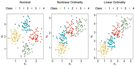
The 2D toy datasets from four classes that are nominal, non-linearly ordinal and linearly ordinal, respectively

With the development of modern technology, high-throughput platforms are providing a large repository of data to facilitate the biomedical research. Among many biomarkers, gene expressions have been known to be powerful predictive features in predicting clinical response. Especially, as the advent of pharmacogenetics suggests, the genomic markup of a patient is believed to have significant influence on medication response, such as disease prognosis and drug toxicity, which will help clinicians prescribe personalized treatment for patients (Duffy and Crown, 2008). In this article, we use gene expressions of patients with multiple myeloma (MM) in two datasets to predict the ordinal level of their drug responses. MM is a type of cancer that is characterized by the proliferation of bone marrow of plasma cells (Terragna et al., 2016). Like other cancers, genetic abnormalities play an essential role in the acquisition of MM. Although it is a relatively uncommon cancer, the overall 5-year survival rate is only 54$\%$⁠. According to the American Cancer Society, roughly 32 270 new cases will be diagnosed and also 12 830 deaths are expected to occur due to MM in 2020. Modern treatments, such as induction, consolidation and maintenance therapy for MM have emerged over the years (Terragna et al., 2016). However, the prognosis of MM still remains variable, partly due to the heterogeneity of patients’ response to the treatments. A number of clinical and laboratory features have been used as a predictive tool for conventional treatment, however, they often fail to identify patients with high risk in the modern therapies (Mulligan et al., 2007).

Both of the two datasets, we will analyze in this work have a large number of predictors $p$ relative to the number of observations $n$⁠. When $p\gg n$⁠, many classical ordinal regression methods are no longer applicable. While there is an abundant amount of research on high-dimensional classification, relatively scarce attention has been paid on ordinal classification with high dimension, low sample size (HDLSS) data. Our methodological contribution in this work is a new ordinal classification method for HDLSS data that has the following advantages: (i) the true ordinal structure will be learned from the data, including irregular or non-linear ordinality; (ii) one can visualize the estimated ordinality by projecting data onto a low-dimensional discriminant space; (iii) the method is scalable in the sense that it can run with HDLSS data as well as low-dimensional data; and (iv) it uses only important features that are relevant for predicting ordinal labels. We employ the concept of ‘feature weighting’ in machine learning (Cardie and Nowe, 1997) into linear discriminant analysis (LDA) (Fisher, 1936), which has been shown to be an effective framework in HDLSS classification literature. With feature weighting, we would consider features that are concordant with the ordinal information with a higher priority than those that are not. Also we employ the group Lasso penalty to achieve a sparse solution for better interpretation. The rest of the ARTICLE is organized as the following: we review existing works and introduce the methodology in Section 2. In Section 3, we discuss the applications on predicting ordinal drug responses based on gene expressions of MM patients and compare the performance of different methods. We also discuss the biological insights revealed by the proposed method. Finally, we conclude with some discussions in Section 4.

2 Materials and methods

2.1 Related work

One of the most naive approaches for ordinal classification is to treat the response as a numerical variable (such as 1, 2, 3, 4 and 5) and fit a regression model. However, this approach would be sensitive to the numerical representations of the labels, which are arbitrarily determined in most cases. In particular, it may be unreasonable to assume equal distancing between adjacent labels. Classical ordinal regression methods, such as the proportional odds model (McCullagh, 1980) and the forward and backward continuation ratio model (Ananth and Kleinbaum, 1997) assume a common covariates effect between adjacent categories under a multinomial logistic regression. A similar idea has been applied to support-vector machines, by assuming parallel maximum margin separating hyperplanes between the adjacent classes (Chu and Keerthi, 2005; Herbrich et al., 1999; Shashua and Levin, 2003).

Some have suggested decomposing a $K$-class classification problem into $K-1$ binary problems. Frank and Hall (2001) considered discriminating a class with label less than $j$ versus no less than $j$⁠. When $K=4$⁠, three binary classifiers will be built on the three binary classifications: $\left\{C_1\right\}$ versus $\{C_2,C_3,C_4\}$⁠, $\{C_1,C_2\}$ versus $\{C_3,C_4\}$ and $\{C_1,C_2,C_3\}$ versus $\left\{C_4\right\}$⁠. Even though this approach takes into account the innate ordinality and enjoys the convenience of using any binary classifiers, at the same time it inevitably increases the computing complexity and introduces multiple modeling errors. Also the prediction can be ambiguous due to crossings of classification boundaries (Qiao, 2017). Another way to modify a regular classification method for ordinal outcomes is to make use of a cost function. Kotsiantis and Pintelas (2004) set the relative cost of misclassifying class $i$ to class $j$ (or vice versa) to be a function of $|i-j|$ so that misclassification to nearer classes will be less penalized than one to farther classes. A similar idea has been implemented in machine learning by Piccarreta (2001) and also in deep learning (de La Torre et al., 2018).

For ordinal classification with HDLSS data, such as drug response prediction, machine learning approaches like k-nearest neighbors and neural networks have been considered (Vougas et al., 2019), however, the ordinality of the classes were not taken into account in their work. Some treated the multi-level ordinal drug response as nominal or combine categories to reduce to a binary classification problem (such as responders versus non-responders or sensitive versus resistance) (Falgreen et al., 2015; Geeleher et al., 2014; Ma et al., 2006), which clearly failed to model the progressing nature of drug response. Another line of work is to regularize classical ordinal regression approaches in order to use them for HDLSS problems. For example, Archer et al. (2014) applied Lasso to a continuation ratio model; Leha et al. (2013) applied the ‘twoing’ idea to ordinal classification with gene expressions; Zhang et al. (2018) proposed a hierarchical ordinal regression to predict the ordinal drug response with gene expression profile for MM patients. However, this line of approaches assume a strict ordinality among the classes, in other words, they all assume that the classes are linearly aligned in the predictor space.

2.2 Proposed methodology

We use $X$ to denote an $n\times p$ input data matrix, with $n$ observations and $p$ predictor variables. Let $X_{n\times p}={({\mathbf{x}}_1^T,\dots ,{\mathbf{x}}_n^T)}^T=({\tilde{\mathbf{x}}}_1,\dots ,{\tilde{\mathbf{x}}}_p)$⁠, where ${\mathbf{x}}_i\in R^p$ is the $i$th row representing the $i$th observation and ${\tilde{\mathbf{x}}}_j\in R^n$ is the $j$th column for the $j$th variable. Each observation falls into one of the $K$ ordinal classes $C_k$⁠, $k\in \{1,\dots ,K\}$ and $C_k$ inherits the natural ordering where $C_1\prec \cdots \prec C_K$ (⁠$\prec$ denotes the ordering). We use $\mathbf{y}={(y_1,\dots ,y_n)}^T$ to denote the vector which contains the class labels, with $y_i\in \{1,\dots ,K\}$⁠.

Suppose that the $j$th variable ${\tilde{\mathbf{x}}}_j$ has a mixture distribution with $K$ components with component means ${\mu }_{1j},\dots ,{\mu }_{Kj}$⁠. We call ${\tilde{\mathbf{x}}}_j$ order-concordant if the component means are monotonically increasing or decreasing with class labels, i.e. ${\mu }_{1j}\le \cdots \le {\mu }_{Kj}$ or ${\mu }_{1j}\ge \cdots \ge {\mu }_{Kj}$⁠. Otherwise they are order-discordant. We naturally assume that order-concordant variables are likely to be more related to the ordinal information than order-discordant ones. Thus, we propose to use the absolute value of the rank correlation between ${\tilde{\mathbf{x}}}_j$ and the class labels $\mathbf{y}$⁠, i.e. $w_j=|\text{rank} \text{corr}({\tilde{\mathbf{x}}}_j,\mathbf{y})|$ as the weight for the $j$th variable. A rank correlation measures the ordinal association between two quantities. Here, we consider two types of rank correlations. First, Spearman’s rank correlation between $Z$ and $Q$ is the Pearson correlation between the ranked variables $\mathit{rgZ}$ and $\mathit{rgQ}$⁠, where $\mathit{rgZ}$ and $\mathit{rgQ}$ are rankings of the original variables, respectively. Second, Kendall’s $\tau$ between $Z$ and $Q$ is the ratio of the number of concordant and discordant pairs: $\tau =\frac{2}{n(n-1)}\times \{(\text{no}.\text{ofconcordantpairs})-(\text{no}.\text{ofdiscordantpairs})\}$⁠, where the pair $(z_i,q_i)$ and $(z_j,q_j)$ (⁠$i\cancel{=}j$⁠) is said to be concordant if $z_i>z_j$ and $q_i>q_j$ or $z_i<z_j$ and $q_i<q_j$ holds, and otherwise discordant. When there is a perfect monotonic relationship between the two sets of variables, both Spearman’s rank correlation and Kendall’s $\tau$ will be $+1$ or $-1$⁠, depending on the direction of the association.

We propose to incorporate the feature weights into the framework of LDA, which is well-known for its robustness and simplicity. LDA aims to project the data onto a low-dimensional discriminant subspace such that the projected data are best separated, in the sense that it achieves maximum between-class covariance and minimum within-class covariance. Assume that the $k$th class have the mean vector ${\mathit{\mu }}_k$ and a common covariance ${\Sigma }_w$⁠, for $k\in \{1,\dots ,K\}$⁠. Then, the set of vectors $({\mathit{\beta }}_1,\dots ,{\mathit{\beta }}_{K-1})$ that span the LDA subspace can be obtained by the following optimization problem:

$$\begin{array}{cc}{{\displaystyle \underset{{\mathit{\beta }}_l\in R^p}{\max }}}_{}\hspace{1em}\hfill & {\mathit{\beta }}_l^T{\Sigma }_b{\mathit{\beta }}_l,\hfill \\ \text{subject} \text{to}\hspace{1em}\hfill & {\mathit{\beta }}_l^T{\Sigma }_w{\mathit{\beta }}_l=1,\hfill \\ \hfill & {\mathit{\beta }}_l^T{\Sigma }_w{\mathit{\beta }}_s=0,\forall \hspace{0.17em}s<l,\hfill \end{array}$$

(1)

where ${\Sigma }_b$ is the between-class covariance matrix that could be estimated as ${\widehat{\Sigma }}_b={\sum }_{k=1}^K\frac{n_k}{n}({\widehat{\mathit{\mu }}}_k-\overline{\mathbf{x}}){({\widehat{\mathit{\mu }}}_k-\overline{\mathbf{x}})}^T$ and ${\Sigma }_w$ could be estimated as ${\widehat{\Sigma }}_w=\frac{1}{n-K}{\sum }_{k=1}^K\sum _{y_i=k}({\mathbf{x}}_i-{\widehat{\mathit{\mu }}}_k){({\mathbf{x}}_i-{\widehat{\mathit{\mu }}}_k)}^T$⁠, with $\overline{\mathbf{x}}$ being the global mean vector and $n_k$ being the number of observations in class $k$⁠.

We can rewrite (1) so that the objective is to find a matrix $B=[{\mathit{\beta }}_1,\dots ,{\mathit{\beta }}_d]$⁠, for a given $(\text{HTML} \text{translation} \text{failed})$ that optimizes

$${{\displaystyle \underset{B\in R^{p\times d}}{\max }}}_{}\text{trace}(B^T{\Sigma }_{b}B),\hspace{1em}\text{subject} \text{to}\hspace{1em}{B}^T{\Sigma }_{w}B=I_d,$$

which leads to the following generalized eigenvalue problem (GEP):

$${\Sigma }_{b}B={\Sigma }_{w}BD,$$

(2)

where $D$ is a diagonal matrix containing the generalized eigenvalues. To solve (2), we need to calculate ${\Sigma }_w^{-1}$⁠, which does not exist when $p>n$⁠. In order to solve this singularity issue, the regularized ridge-type LDA (Friedman, 1989) was proposed to replace ${\widehat{\Sigma }}_w$ by ${\widehat{\Sigma }}_w+\alpha I_p$ for $\alpha >0$⁠. We propose a regularization that incorporates the weights by using $\alpha \overline{W}$ instead, where ${\overline{W}}_{p\times p}$ is the diagonal matrix containing ${\overline{w}}_j=1-w_j$ and $w_j$’s are (standardized) absolute rank correlations discussed above. The objective function of this feature-weighted LDA is given as:

$${{\displaystyle \underset{B\in R^{p\times d}}{\max }}}_{}\text{trace}(B^T{\Sigma }_{b}B),\hspace{1em}\text{subject} \text{to}\hspace{1em}{B}^T({\Sigma }_w+\alpha \overline{W})B=I_d,$$

(3)

where $\alpha >0$⁠, whose solution satisfies the following GEP

$${\Sigma }_{b}B=({\Sigma }_w+\alpha \overline{W})BD.$$

(4)

Once (3) is solved, we project the data onto the column space of $B$⁠, and apply the standard LDA for class assignment. We note that if $\overline{W}$ is replaced by a ‘roughness’ penalty matrix, this approach can be seen as the penalized LDA (PLDA) by Hastie et al. (1995), who also showed the equivalence to a penalized optimal scoring. Thus, it can be shown that the feature-weighted LDA is equivalent to finding ${\mathit{\beta }}_1,\dots ,{\mathit{\beta }}_k$ that are solutions to the following:

$$\begin{array}{cc}{{\displaystyle \underset{\mathit{\theta }\in R^K,\hspace{0.17em}\mathit{\beta }\in R^p}{\min }}}_{}\hfill & \frac{1}{n}\left\{\right||Y\mathit{\theta }-X\mathit{\beta }|{|}_2^2+{\mathit{\beta }}^T(\alpha n\overline{W})\mathit{\beta }\},\hfill \\ \hspace{1em}\text{subject} \text{to}\hspace{1em}\hfill & \frac{1}{n}{\mathit{\theta }}^T{Y}^{T}Y\mathit{\theta }=1,\hfill \end{array}$$

(5)

where $Y$ is an $n\times K$ indicator matrix whose columns corresponds to the dummy coding of the $K$ classes and $\mathit{\theta }$ is the scoring vector in optimal scoring. From (5), it can be shown that $\overline{W}$ is actually imposing penalties on $\mathit{\beta }$’s, such that a smaller ${\overline{w}}_i$ (corresponding to a larger rank correlation) will push the coefficient to be penalized less compared to one with a larger ${\overline{w}}_i$⁠.

When $p$ is large, feature selection is essential for the interpretability of the results. In order to achieve a sparse solution for feature-weighted LDA, we add a group LASSO penalty (Yuan and Lin, 2006) on the GEP (4). Jung et al. (2019) proposed a framework for sparse GEP and suggested two algorithms to find a solution, namely penalized orthogonal iteration (POI) and fast-POI. Here, we apply the fast-POI algorithm to solve (4) with a group LASSO penalty: $p_{\lambda }(B)=\lambda {\sum }_{i=1}^p\left|\right|{\mathbf{b}}_i|{|}_2$⁠, with ${\mathbf{b}}_i$ being the $i$th row of $B$⁠. The advantage of group LASSO over LASSO is that the former can achieve the sparsity at a group level. That is, whether or not a predictor will be dropped out of the model is consistent for all the dimensions in the discriminant subspace. A sparse estimate of $B$ can be obtained by solving the following:

$${{\displaystyle \underset{B\in R^{p\times d}}{\min }}}_{}\hspace{0.17em}\hspace{0.17em}\text{trace}\{\frac{1}{2}{B}^T({\Sigma }_w+\alpha \overline{W})B-B^{T}V\}+\lambda \sum _{i=1}^p\left|\right|{\mathbf{b}}_i|{|}_2,$$

(6)

where $V$ is a $p\times d$ matrix whose columns are the eigenvectors of ${\Sigma }_b$ corresponding to the $d$ largest eigenvalues of ${\Sigma }_b$⁠, and $\lambda >0$ is a parameter that controls the sparsity. We name this approach the feature-weighted ordinal classification (FWOC).

To solve (6), we apply the block coordinate descent algorithm, which updates one coordinate at a time. The $i$th row of $B$⁠, given ${\mathbf{b}}_j$ is fixed (⁠$j\cancel{=}i$⁠), is updated as the following until convergence:

$${\mathbf{b}}_i=\frac{1}{s_{ii}}{\left(1-\frac{\lambda }{\left|\right|{\mathbf{q}}_i|{|}_2}\right)}_{+}{\mathbf{q}}_i,$$

where $s_{ii}$ is the $i$th diagonal element of $({\Sigma }_w+\alpha \overline{W})$⁠, ${\mathbf{q}}_i={\mathbf{v}}_i-\sum _{i\cancel{=}j}{b}_{ij}{\mathbf{b}}_j$ and ${\mathbf{v}}_i$ is the $i$th row of $V$⁠.

2.3 Tuning parameters

In the actual implementation, we re-parameterize so that ${\Sigma }_w+\alpha \overline{W}$ is replaced by $r{\Sigma }_w+(1-r)\overline{W}$ so that the tuning range is bounded within $[0,1]$⁠. Clearly $r$ controls how much the classifier depends on the ordinal information, in the sense that $r\approx 1$ will yield the method more focused on maximizing the separation of the classes without regard to the ordinality. On the contrary, $r\approx 0$ will yield a solution more dependent on order-concordant variables than discordant ones for classification. We propose to learn a good compromise from the data in order to obtain an efficient classifier that reflects the ordinality. Another parameter $\lambda$ controls the sparsity of the solution. A larger $\lambda$ imposes a heavier penalty on the solution thus yields a more sparse solution. Note that, there is a upper bound of $\lambda$ that gives a non-trivial solution to (6), which can be shown to be ${\lambda }_{\mathit{max}}={\max }_{i\in \{1,\dots ,p\}}\left|\right|{\mathbf{v}}_i|{|}_2$⁠.

We use the $5$-fold cross-validation to select the optimal tuning parameters $(r_{\mathit{opt}},{\lambda }_{\mathit{opt}})$⁠, based on a grid search. When there are ties in the grid space. we adopt a parsimonious rule of selecting the most sparse and ordinal solution, which favors larger $\lambda$ and smaller $r$⁠. As for the model evaluation used for cross-validation, we use Kendall’s $\tau$ between the predicted and actual labels.

3 Drug response prediction for MM

In this section, we test our high-dimensional ordinal classification method FWOC using the datasets from Mulligan et al. (2007) and Terragna et al. (2016), which correspond to GSE9782 and GSE68871 in the Gene Expression Omnibus database, respectively. The GSE9782 dataset was generated using the Affymetrix HG-U133 A/B platform and consists of 169 pre-treated tumor cell samples from the patients with relapsed myeloma who were enrolled in the Phase 2 and Phase 3 clinical trials of bortezomib. The GSE68871 dataset was generated using the Affymetrix HG-U133 Plus 2.0 Array and consists of 118 primary tumor cell samples obtained from new MM patients who received the bortezomib-thalidomide-dexamethasone (VTD) induction therapy. A summary of the two datasets is in Table 1. Both of the two datasets have five ordinal outcomes (drug response). Note that, the observed proportions are severely unbalanced in either dataset.

Table 1.

Summary of the two datasets with ordinally recorded drug responses

Dataset	GSE9782	GSE68871
Sample size	169	118
No. of probes	22 283	54 675
	1 Complete response (CR)	Complete response (CR)
	(⁠$7.69\%$⁠)	(⁠$12.71\%$⁠)
	2 Partial response (PR)	Near complete response (NCR)
	(⁠$35.50\%$⁠)	(⁠$11.86\%$⁠)
Outcome	3 Minimal response (MR)	Very good partial response (VGPR)
	(⁠$7.10\%$⁠)	(⁠$33.90\%$⁠)
(Class-size)	4 No change (NC)	Partial response (PR)
	(⁠$25.44\%$⁠)	(⁠$35.59\%$⁠)
	5 Progressive disease (PD)	Stable disease (SD)
	(⁠$24.26\%$⁠)	(⁠$5.93\%$⁠)

We consider the following three methods to compare with the proposed FWOC: Archer et al. (2014), Zhang et al. (2018) and Witten and Tibshirani (2011). Archer et al. (2014) incorporated Lasso in continuation ratio model, and proposed the following

$${{\displaystyle \underset{\mathit{\beta }\in R^p}{\max }}}_{}\hspace{0.17em}\hspace{0.17em}\hspace{0.17em}L(\mathit{\beta }|\mathbf{y},\mathbf{x})-\lambda \sum _{i=1}^p|{\beta }_i|,$$

(7)

where $L(\mathit{\beta }|\mathbf{y},\mathbf{x})$ denotes the likelihood for the continuation ratio model and $\lambda$ is the parameter controlling the degree of $L_1$ penalty. We call their method PCRM (penalized continuation ratio model) in this work. Zhang et al. (2018) proposed the following a multi-variable ordinal model called BhGLM:

$$P(y_i=k)=\{\begin{array}{cc}1-{\text{logit}}^{-1}({\mathbf{x}}_i^T\mathit{\beta }-c_1),\hfill & \hfill \text{for}\hspace{0.17em}k=1\\ {\text{logit}}^{-1}({\mathbf{x}}_i^T\mathit{\beta }-c_{k-1}),\hfill & \hfill \text{for}\hspace{0.17em}k=K\\ {\text{logit}}^{-1}({\mathbf{x}}_i^T\mathit{\beta }-c_{k-1})-{\text{logit}}^{-1}({\mathbf{x}}_i^T\mathit{\beta }-c_k),\hfill & \hfill \mathrm{o}.\mathrm{w}.\end{array}$$

in which a Cauchy prior was applied on the coefficients for sparsity. Note that both of PCRM and BhGLM are model-based approaches that assume linearly ordered classes. The third method by Witten and Tibshirani (2011) is a well-known multi-class sparse LDA that was originally developed for nominal multi-category classification. They added a penalty function in the framework of the LDA to propose an optimization criterion given as:

$$\begin{array}{cc}{{\displaystyle \underset{{\mathit{\beta }}_l\in R^p}{\max }}}_{}\hspace{0.17em}\hspace{0.17em}\hfill & {\mathit{\beta }}_l^T{\Sigma }_b{\mathit{\beta }}_l-P_1({\mathit{\beta }}_l),\hfill \\ \text{subject} \text{to} \hspace{1em}\hfill & {\mathit{\beta }}_l^T{\tilde{\Sigma }}_w{\mathit{\beta }}_l\le 1,\hfill \\ \hfill & {\mathit{\beta }}_l^T{\tilde{\Sigma }}_w{\mathit{\beta }}_s=0,\hspace{1em}\forall \hspace{0.17em}s<l\hfill \end{array},$$

(8)

where $P_1({\mathit{\beta }}_l)$ is a convex penalty on ${\mathit{\beta }}_j$⁠, such as the Lasso penalty, and ${\tilde{\Sigma }}_w$ is a positive estimate of ${\Sigma }_w$⁠, such as ${\Sigma }_w+\lambda \Omega$ or a diagonal estimate. We call this method PLDA in this work. Both FWOC and PLDA are projection-based approaches, in that they both aim to project the data onto a lower-dimensional discriminant subspace and then apply the standard classification methods (such as LDA) on the projected data to assign class memberships.

For each of the two datasets, we randomly split it into a training set with $70\%$ observations and a test set with $30\%$ observations and repeated the random split for 10 times. In each repetition, we pre-screened the probes using the univariate ordinal logistic regression model (Zhang et al., 2018) within the training set. Then, we applied the four methods and evaluated the performance on the test set. The number of probes pre-screened for GSE9782 and GSE68871 are 500 and 1000, respectively, for the probes in GSE68871 are about twice many as GSE9782. In implementing FWOC, we used Kendall’s $\tau$ for the feature weights. For FWOC and PLDA, the dimension of the discriminant subspace is set to be two, considering the ordinality of the classes.

3.1 Results

Table 2 reports the classification accuracy, Kendall’s $\tau$ and weighted cost between predicted and actual labels, and the number of selected probes from the four methods, averaged over 10 repetitions. The weighted cost is defined as: $\sum |y_i-f({\mathbf{x}}_i){|}^m,$ where $f({\mathbf{x}}_i)$ is the predicted class label and $m$ is a positive integer. We use $m=1$ here. Even though all four methods are supposed to be sparse methods, the numbers of selected probes are wildly different. Both BhGLM and PLDA use (almost) all variables for constructing a classifier where PCRM selects the least number of probes. FWOC shows a moderate degree of sparsity. Also its classification accuracy and Kendall’s $\tau$ are the highest for both data and its weighted cost is the lowest or the second lowest. This implies that its drug response predictions are most accurate and at the same time consistent with the hierarchy of the response levels.

Table 2.

Prediction results of drug responses of MM patients

Dataset	Metric	FWOC	BhGLM	PCRM	PLDA
GSE9782	Classification accuracy	0.396	0.367	0.369	0.388
		(0.015)	(0.018)	(0.018)	(0.019)
	Kendall’s $\tau$	0.300	0.240	0.218	0.257
		(0.029)	(0.027)	(0.043)	(0.035)
	Weighted cost	1.056	1.135	1.250	1.121
		(0.028)	(0.035)	(0.063)	(0.048)
	No. of selected probes	239.1	500	112.8	496.3
		(14.601)	(0)	(2.670)	(2.155)
GSE68871	Classification accuracy	0.444	0.388	0.374	0.344
		(0.027)	(0.027)	(0.023)	(0.013)
	Kendall’s $\tau$	0.311	0.292	0.217	0.246
		(0.015)	(0.049)	(0.035)	(0.024)
	Weighted cost	0.806	0.785	0.941	0.888
		(0.024)	(0.036)	(0.049)	(0.023)
	No. of selected probes	162	1000	76	1000
		(40.210)	(0)	(1.741)	(0)

Note: Averages of classification accuracy, Kendall’s $\tau$⁠, weighted cost between predicted and actual outcomes and the number of selected probes are shown with standard errors in parentheses.

We visualize the results with bar graphs in Figures 2 and 3. In each gray-scale bar, the darker the gray color is, the nearer the predicted class is to the true one, with the overall length equal to the observed counts of the class in the data. With these figures, we can know the details about classification patterns of the methods, especially with regard to the challenges due to the unbalanced class proportions. Figure 2 reveals that for GSE9782, PLDA, PCRM and FWOC are best in exactly classifying Classes 2, 4 and 5 respectively. If we consider the misclassification to neighboring classes as an ‘acceptable error’, we find that FWOC is clearly the best, which is also implied by its highest Kendall’s $\tau$ in Table 2. The results for GSE68871 in Figure 3 show that FWOC achieved the most correct classification for Classes 1, 2, 4 and 5 while BhGLM is better for Class 3. It is noticeable that the three compared methods, BhGLM, PCRM and PLDA, are particularly worse in the smaller classes. We also observed that they tended to assign samples to larger classes, which may create a bias when trained with unbalanced data.

Fig. 2.

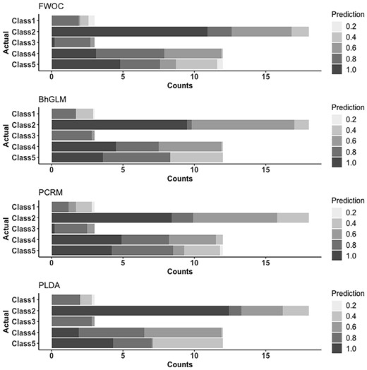
A detailed view on out-of-sample predictions for GSE9782 data. Each bar, representing the observed counts of each class, is partitioned according to the proximity of the predicted classes. The scales of gray color are determined by $1-|i-j|/5$⁠, where $i$ and $j$ are the label for the actual class and predicted class, respectively. For instance, in the first bar plot for FWOC, we can see that there are 12 cases of Class 4 in the data, out of which about 3 cases (averaged from 10 repeated trainings) are correctly classified to Class 4, 5 cases are classified to neighboring classes (3 or 5), and 4 cases are classified to Class 2

Fig. 3.

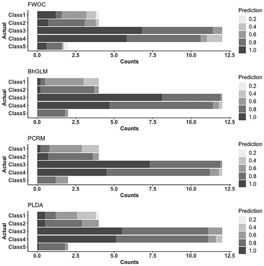
A detailed view on out-of-sample predictions for GSE68871 data

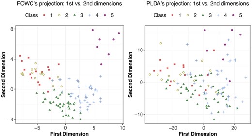
As discussed in Section 2, both FWOC and PLDA estimate a discriminant subspace, onto which we can project the data to see the pattern of classes. The 2D projections obtained from FWOC and PLDA are in Figures 4 and 5 for GSE9782 and GSE 68871, respectively. The left panel in Figure 4 shows much better class separation than the right one. More importantly, it reveals that the classes have a non-linear ordinality and one dimension is not sufficient to separate the classes, which implies that assuming a strictly linear ordinality may not be appropriate. Furthermore, we see that Class 3 (MR) and Class 4 (NC) are close to each other compared with the other three classes, which indicates that the pathological difference between ‘no change’ and ‘minimum response’ to Bortezomib therapy may be small, or that one cannot distinguish them well based on gene expressions. The projections for GSE68871 data in Figure 5 show a similar pattern. We can see that Classes 1 and 2 are heavily overlapped, which similarly implies that the pathological difference between ‘complete response’ and ‘near complete response’ to the VTD therapy may be negligible.

Fig. 4.

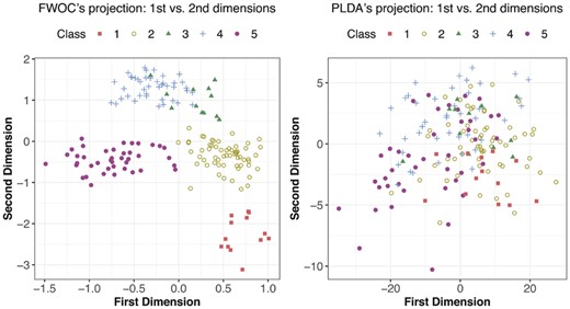
Projections of GSE9782 data onto the 2D discriminant subspace obtained by FWOC and PLDA

Fig. 5.

Projections of GSE68871 data onto the 2D discriminant subspace obtained by FWOC and PLDA

3.2 Gene-wise interpretation

In this section, we take a closer look at the probes selected by our proposed method. Specifically, we chose the top 50 probes with the largest $L_1$ norm of $B$⁠. Figure 6 shows the heatmap for the top 50 probes for GSE9782, with each row corresponding to a patient. Note that, the probes in the x-axis are re-arranged so that similar patterns are easy to be detected. Most of the top 50 probes are clearly over-expressed for patients who did not respond well to the drug, while other probes show the opposite pattern. Common molecular functions from gene ontology (GO) of the top genes: protein binding, poly(A) RNA binding, RNA binding, structural constituent of ribosome, nucleotide binding and ATP binding. Protein binding is known to affect drug activity, either by changing the effective concentrations or by affecting the lasting time of the effective concentrations (Keen, 1971). Further, many of the probes are from the ribosomal protein gene family (RPL15, RPL10A, RPS5, RPL22, RPL35A, RPL38, etc.), some genes are related with ATP synthase, H+ transporting (ATP5O, ATP5L, ATP5S, ATP5SL, ATP5G2) and eukaryotic translation initiation factor 3 (EIF3D, EIF3K). Ribosomal protein has been shown to be a novel oncogenic driver, in which the defect of ribosomal may break the balance of protein production. What is more, bortezomib, as a type of proteasome inhibitors, is shown to be a promising treatment for ribosome-defective cancer (Sulima and De Keersmaecker, 2017) and such therapies may benefit patients with various ribosomal defect. Therefore, ribosomal-related activities are sensitive to the treatment of bortezomib. In addition, the translation initiation factors are also related with treatment to MM (Zismanov et al., 2015).

Fig. 6.

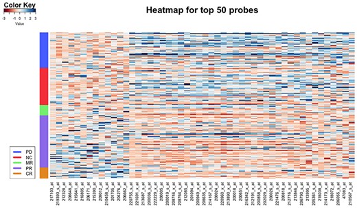
Heatmap for the top 50 probes selected by FWOC from GSE9782. Each row represents a sample and each column represents a probe

From the heatmap for GSE68871 in Figure 7, it is clear that gene expression levels of the selected probes also show a pattern that corresponds to the monotonic change of class labels. With regard to GO, we have found that the top genes cover various functions that are related with the development of mutliple myeloma, such as immunoglobulin heavy constant gamma (Bergsagel et al., 1996), fas cell surface death receptor (Yu and Li, 2013), long intergenic non-protein coding (Butova et al., 2019) and so on. What is more, the most significant biological process found via gene set analysis is positive regulation of peroxisome proliferator-activated receptor signaling pathway, which has been shown to be related to the apoptosis of MM cells (Garcia-Bates et al., 2008). Also, it is known that the inhibition of drug-induced cell apoptosis is closely related with drug resistance in myeloma (Vougas et al., 2019).

Fig. 7.

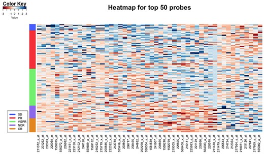
Heatmap for the top 50 probes selected by FWOC from GSE68871. Each row represents a sample and each column represents a probe

4 Conclusion

In this article, we proposed a novel FWOC method, which incorporates the feature weights into the framework of sparse LDA to obtain an effective classifier that accounts for the ordinality. Unlike traditional approaches that assume a certain ordinal structure, such as linear, projection to FWOC subspace can visualize the learned structure of ordinality. Our study on MM has revealed that the drug response categories are indeed non-linear.

A motivation behind this work came from an empirical observation in many HDLSS sparse classification studies. We have found that often a multiple number of classifiers would yield similarly good classification accuracies even when there is hardly no overlap in the sets of chosen features. When the labels are ordinal, we can reduce this ambiguity by making use of a key information in the data that are often overlooked: ordinality of the labels. Clinicians are more likely to prefer a drug response prediction model that reflects the progressing nature of the response categories, biologically or functionally, than a model built to only predict the exact level of response without regard to their natural hierarchy in the labels. Thus, when the classification accuracies are comparable, a classifier depending more on the variables that are correlated with the ordinality should be preferred.

For both MM studies, we used the dimension of the discriminant subspace $d=1$⁠. As the number of ordinal classes is $K=5$ for either dataset, the range of the dimension $d$ of the discriminant subspace is $[1,4]$⁠. We recommend 2 or 3 for a problem like this, as it balances between a complete nominal case (⁠$d=4$⁠) and a strictly linear case (⁠$d=1$⁠). Even though omitted in the manuscript, we did try both dimensions found that they are similar in terms of prediction accuracy. As it is easier to graphically present the estimated subspace with $d=2$ than $d=3$⁠, we chose to present the result. One of the compared methods, PLDA, actually tuned the dimension and in most of the trainings, $d$ was estimated to be 2 or 3.

Asked by reviewers, we conducted an extensive simulation study with various ordinality structures and underlying covariance types. We have found that the proposed approach is competitive in all settings and particularly advantageous when the classes are non-linearly ordered and variables are meaningfully correlated. The details on this study are available in the Supplementary Material.

We note that, there are other ways to incorporate the feature weighting into the LDA framework, which we will leave as an immediate future work. First, one can use a different weight function. For example, univariate isotropic regression can be used to determine which feature is significantly order-concordant. Second, one can use an alternative LDA formulation, such as optimal scoring to set up a regression-type optimization problem, which might open up more ways to incorporate the feature weights.

Financial Support: none declared.

Conflict of Interest: none declared.