Sparse least trimmed squares regression with compositional covariates for high-dimensional data

Abstract

Motivation

High-throughput sequencing technologies generate a huge amount of data, permitting the quantification of microbiome compositions. The obtained data are essentially sparse compositional data vectors, namely vectors of bacterial gene proportions which compose the microbiome. Subsequently, the need for statistical and computational methods that consider the special nature of microbiome data has increased. A critical aspect in microbiome research is to identify microbes associated with a clinical outcome. Another crucial aspect with high-dimensional data is the detection of outlying observations, whose presence affects seriously the prediction accuracy.

Results

In this article, we connect robustness and sparsity in the context of variable selection in regression with compositional covariates with a continuous response. The compositional character of the covariates is taken into account by a linear log-contrast model, and elastic-net regularization achieves sparsity in the regression coefficient estimates. Robustness is obtained by performing trimming in the objective function of the estimator. A reweighting step increases the efficiency of the estimator, and it also allows for diagnostics in terms of outlier identification. The numerical performance of the proposed method is evaluated via simulation studies, and its usefulness is illustrated by an application to a microbiome study with the aim to predict caffeine intake based on the human gut microbiome composition.

Availability and implementation

The R-package ‘RobZS’ can be downloaded at https://github.com/giannamonti/RobZS.

Supplementary information

Supplementary data are available at Bioinformatics online.

1 Introduction

Human microbiome studies that make use of high-throughput technologies are a valuable source of information for the human health. The human microbiome, constituted by all microorganisms in and on the human body, is associated to health and has an impact on risk of disease. A microbiome dataset, derived from 16S rRNA sequencing, consists in the collection of abundances of microbial operational taxonomic units (OTUs), or bacterial taxa. Such count data are usually normalized by the total abundance of a sample to relative abundances, to account for differences in sequencing depths. In that case, the values of each observation would sum up to 1 or 100%, if reported in proportions or percentages, and many statistical methods such as regression on the normalized data are no longer applicable because of data singularity.

In the literature, microbiome data have been considered and successfully treated as compositional data (CODA) (Li, 2015; Gloor et al., 2016; Quinn et al., 2018). CODA convey relative information in a sense that the (log-)ratios of the values between the variables are of major interest for the analysis (Filzmoser et al., 2018). This leads to many appealing properties, one of them being scale invariance: the ratios between the original or between the relative abundances are identical, and thus the statistical analysis does not depend on how the data are normalized, or if they are normalized at all. The lack of scale invariance is also a major argument against applying standard regression models on the original data, even if the data have not been normalized to constant sum.

In many studies, the microbiome composition is used as covariate in regression models to analyze its association with a clinical outcome. This composition has special features: it consists of many variables and thus forms high-dimensional data. Many abundances are reported as zero, and thus we can talk about sparse data. Typically, only few variables from the composition are important to model the outcome, and most of them are irrelevant for the model. Thus, an appropriate variable selection is desirable and necessary. A further challenge are data outliers, i.e. observations which deviate from the majority of the samples. In the ideal case, outlying observations should receive smaller weight in the regression problem in order to reduce their influence on the estimated regression coefficients. Robust regression methods take care of an appropriate weighting scheme (Maronna et al., 2006).

In this article, we propose a unified framework capable to integrate robust techniques in the context of the variable selection and coefficient estimation problem in high-dimensional regression with compositional covariates, leading to parsimonious inferential solutions and models which are easier to interpret.

Several methods to perform regression with compositional exploratory variables have been presented in the literature: for a mixture experiment, Aitchison and Bacon-Shone (1984) introduced a CODA regression model based on linear log-contrasts, namely a linear combination of logratios between compositional parts.

In the high-dimensional setting, Lin et al. (2014) considered variable selection and estimation for the log-contrast model. They proposed an ${\ell }_1$ regularization method for the linear log-contrast regression model with a linear constraint on the coefficients. Their constrained Lasso is also known as ZeroSum regression, it incorporates the compositional nature of the data into the model, and works well in the high-dimensional setting where the number of available regressors p is much larger than the number of observations n. Shi et al. (2016) extended the linear log-contrast regression model by imposing a set of multiple linear constraints on the coefficients in order to achieve subcompositional coherence of the results obtained at different taxonomic ranks which the composition of taxa belongs to. Altenbuchinger et al. (2017) imposed an elastic-net penalty to the ZeroSum regression, developing a coordinate descent algorithm for the estimation. This constrained regularized regression method has been applied in case of compositional covariates, as well as reference point insensitive analyses involving any biological measurement such as the human microbiome.

Bates and Tibshirani (2019) adapted Lasso for CODA, using the logratios of all variable pairs of the components as predictors. They proposed a two-step fitting procedure that combines a convex filtering step with a second non-convex pruning step, yielding highly sparse solutions to face the very large dimensionality of the predictor space.

Some penalized robust estimation methods have been recently proposed in the literature. These include an MM-estimator with a ridge penalty (Maronna, 2011), a sparse least trimmed squares (LTSs) regression estimator with a lasso penalty (Alfons et al., 2013), and with elastic-net penalty (Kurnaz et al., 2018), a regularized S-estimator with an elastic-net penalty (Freue et al., 2019) and bridge MM-estimators (Smucler and Yohai, 2017), among others.

In this article, we propose a robust version of the penalized ZeroSum regression. Robustness is achieved by trimming large residuals, motivated by the fact that outliers in the data affect the inferential results, and also small misspecifications of the underlying parametric model can lead to poor prediction accuracy (Huber and Ronchetti, 2009; Maronna et al., 2006).

The outline of the paper is as follows. Section 2 reviews the regression models with compositional covariates, and presents the Robust ZeroSum regression estimator. Simulation experiments are conducted in Section 3 to evaluate the numerical performance of the proposed method. Section 4 presents an application to gut microbiome data, and the final Section 5 concludes.

2 Regression models for CODA

2.1 Linear log-contrast model

In the seminal work of Aitchison and Bacon-Shone (1984), a regression model for CODA was introduced, which is known as linear log-contrast model. It is related to the design of experiments with mixtures, called simplex designs. Consider a matrix X of compositional covariates, $\mathbf{X}={[x_{ij}]}_{1\le i\le n; 1\le j\le p}$⁠, w.l.o.g. expressed with constant sum 1. Thus, each row lies in the unit simplex ${\mathcal{S}}^p=\{x_{ij}:x_{ij}>0\text{and}{\sum }_{j=1}^p{x}_{ij}=1\}$⁠. The log-transformed values of X are collected in the matrix $\mathbf{Z}={[z_{ij}=\text{log}(x_{ij})]}_{1\le i\le n; 1\le j\le p}\in {\mathbb{R}}^{n\times p}$⁠. A log-contrast is defined, in a symmetric form, as a linear combination of the columns of Z with coefficients $\mathit{\beta }={({\beta }_1,\dots ,{\beta }_p)}^T$⁠, thus $\mathbf{Z}\mathit{\beta }$⁠, with the constraint ${\sum }_{j=1}^p{\beta }_j=0$ (Lin et al., 2014). The linear log-contrast model considers a response with values $\mathbf{y}={(y_1,\dots ,y_n)}^T$⁠, and the corresponding regression model with the log-contrast as covariates is

$$\mathbf{y}=\mathbf{Z}\mathit{\beta }+\mathit{\epsilon },\hspace{0.17em}\text{st}\hspace{0.17em}\sum _{j=1}^p{\beta }_j=0,$$

(1)

where $\mathit{\epsilon }$ is the error component, usually assumed normally distributed around zero, with constant variance ${\sigma }^2$⁠. The parameters are usually estimated by the least-squares (LS) method considering the constraint on the parameters. Note that the formulation (1) does not include an intercept in the model, as it can be omitted by centering all the predictor variables and the response.

In the high-dimensional setting, when the sample size n is lower than the number of predictors p, and the ordinary LSs method is not applicable, Lin et al. (2014) proposed a variable selection procedure and estimation for a sparse log-contrast model,

$${\widehat{\mathit{\beta }}}_{\mathit{sparse}}=\underset{{}_{\mathit{\beta }\in {\mathbb{R}}^p}}{\arg \min }(\frac{1}{n}{\Vert \mathbf{y}-\mathbf{Z}\mathit{\beta }\Vert }_2^2+\lambda {\Vert \mathit{\beta }\Vert }_1),\hspace{0.17em}\text{st}\sum _{j=1}^p{\beta }_j=0,$$

(2)

where $\lambda >0$⁠, is the regularization parameter, which calibrates the sparseness, and ${\Vert ·\Vert }_2$ and ${\Vert ·\Vert }_1$ indicate the ${\ell }_2$ and ${\ell }_1$ norm, respectively. Depending on the choice of λ, several or many of the components of $\mathit{\beta }$ are zero, and thus this sparse regression coefficient vector corresponds to a variable selection in the model. The authors introduced a coordinate descent method of multipliers to estimate the model parameters. By virtue of the zero-sum constraint, the proposed estimator fulfills desirable compositional properties such as scale invariance, i.e. the regression coefficients are independent of an arbitrary scaling of the basis count from which a composition is obtained, permutation invariance and selection invariance. The selection invariance property asserts that the estimator is unchanged if one knew in advance which components would be estimated as zero and applied the procedure only to the components associated to non-zero coefficients (Lin et al., 2014).

Altenbuchinger et al. (2017) combined the variable selection problem and estimation for model (1) with the elastic-net regularization (Zou and Hastie, 2005),

$${\widehat{\mathit{\beta }}}_{\mathit{ZeroSum}}=\underset{{}_{\mathit{\beta }\in {\mathbb{R}}^p}}{\arg \min }(\frac{1}{n}{\Vert \mathbf{y}-\mathbf{Z}\mathit{\beta }\Vert }_2^2+\lambda P_{\alpha }(\mathit{\beta }\left)\right),\hspace{0.17em}\text{st} \sum _{j=1}^p{\beta }_j=0,$$

(3)

where $P_{\alpha }(\mathit{\beta })=(\alpha {\Vert \mathit{\beta }\Vert }_1+\frac{1-\alpha }{2}{\Vert \mathit{\beta }\Vert }_2^2)$ is the elastic-net penalty, $\alpha \in [0,1]$ is a tuning parameter which balances the ${\ell }_2$ and ${\ell }_1$ penalty. Model (3) is known as ZeroSum elastic-net estimator, to emphasize the constraint on the regression coefficients in conjunction with the elastic-net regularization. To fit the model (3), a coordinate descent-based algorithm (Friedman et al., 2007) was implemented. Setting α = 1, model (3) is the Lasso model, and for α = 0 it is Ridge regression (Tibshirani, 1994).

2.2 Robust and sparse regression models for CODA

It is well known that the ordinary LSs estimator for linear regression is very sensitive to the presence of outliers in the space spanned by the dependent variable, namely vertical outliers, and in the space spanned by the regressors, namely leverage points. To overcome this issue, several robust alternatives were proposed in the literature; among others, we focus here on Rousseeuw’s LTS estimator (Rousseeuw, 1984).

Considering a regression of the response y on the design matrix $\mathbf{X}\in {\mathbb{R}}^{n\times p}$⁠, i.e. $\mathbf{y}=\mathbf{X}\mathit{\beta }+\mathit{\epsilon }$⁠, where $\mathit{\beta }={({\beta }_1,\dots ,{\beta }_p)}^T\in {\mathbb{R}}^p$⁠. For every $\mathit{\beta }\in {\mathbb{R}}^p$ we denote the corresponding residuals by $r_i(\mathit{\beta })=y_i-{\mathbf{x}}_i^T\mathit{\beta },\hspace{0.17em}(i=1,\dots ,n)$⁠, where ${\mathbf{x}}_i={(x_{i1},\dots ,x_{ip})}^T$⁠. Denote the ordered squared residuals as $r_{(1)}^2\le \dots \le r_{(n)}^2$⁠, then the LTS estimator is obtained as

$${\widehat{\mathit{\beta }}}_{\text{LTS}}=\underset{{}_{\mathit{\beta }\in {\mathbb{R}}^p}}{\arg \min }(\sum _{i=1}^h{r}_{(i)}^2(\mathit{\beta })),$$

(4)

where h may lie between $n/2$ and n. The specific choice of h depends on the desired properties of the resulting estimator: a smaller value leads to more robustness, but to less efficiency, and vice versa. Minimizing (4) is equivalent to finding the subset of size h with the smallest LSs objective function. As the number of observations and covariates increases, the search of LTS estimates in (4) becomes computationally more and more expensive, and thus a fast-LTS algorithm (Rousseeuw and Van Driessen, 2006) was proposed. The basic idea of this algorithm consists in the concentration-step (C-step), in which the most promising subsets of size h are used to find a local optimum. These C-steps can be repeated a specified number of times, or iterated until convergence.

Alfons et al. (2013) proposed an extension of the fast-LTS algorithm for sparse data by adding an ${\ell }_1$ penalty on the LTS coefficient estimates, leading to the sparse LTS estimator

$${\widehat{\mathit{\beta }}}_{\text{SLTS}}=\underset{{}_{\mathit{\beta }\in {\mathbb{R}}^p}}{\arg \min }(\sum _{i=1}^h{r}_{(i)}^2(\mathit{\beta })+h\lambda {\Vert \mathit{\beta }\Vert }_1),$$

(5)

for $h\le n$ and the tuning parameter $\lambda \ge 0$⁠. Sparse LTS regression is equivalent to detecting the subset of h observations whose Lasso fit leads to the smallest penalized sum of squared residuals. The sparse LTS estimator can be interpreted as a trimmed version of the Lasso. Due to the ${\ell }_1$ penalty, some of the estimated regression coefficients are exactly zero, performing variable selection. Since potential outliers are trimmed in the objective function, the sparse LTS estimator is robust against vertical outliers, and leverage points.

Kurnaz et al. (2018) extended the work of Alfons et al. (2013) by substituting the ${\ell }_1$ penalization in (5) with an elastic-net (EN) penalty. They proposed the trimmed (EN)LTS estimator, defined by

$${\widehat{\mathit{\beta }}}_{\left(\text{EN}\right)\text{LTS}}=\underset{{}_{\mathit{\beta }\in {\mathbb{R}}^p}}{\arg \min }\underset{{}_{\begin{array}{c}H\subseteq \{1,\dots ,n\}:\\ \left|H\right|=h\end{array}}}{\arg \min }(\sum _{i\in H}{(y_i-{\mathbf{x}}_i^T\mathit{\beta })}^2+h\lambda P_{\alpha }(\mathit{\beta })),$$

(6)

where $P_{\alpha }(\mathit{\beta })$ is the elastic-net penalty as in (3), H is an outlier-free subset of the set of all indexes $\{1,2,\dots ,n\}$⁠, and $\left|H\right|$ denotes the cardinality of the set H. They used an analogue of the iterative fast-LTS algorithm along with a ‘warm start’ strategy to obtain the optimal choice of the tuning parameters α and λ in (6).

Our study extends the trimmed (EN)LTS estimator to a constrained parameter space, to convey the zero-sum constraint typical for compositional covariates. We call our estimator the Robust ZeroSum (RobZS) estimator. The interesting aspect of RobZS is the combination of the zero-sum constraint of the regression coefficients, with the elastic-net regularization in a robust way.

The algorithm to find the solution of RobZS is detailed in Section 2.3. The selection of the tuning parameters α and λ will be discussed in Supplementary Section S1 of Supplementary Material, and an extensive simulation study, reported in Section 3, demonstrates the robustness of the estimator in presence of data outliers.

2.3 Algorithm

A preprocessing data step is required: the response variable and the compositional covariates are robustly centered by the median.

Let $\mathcal{R}(H,\mathit{\beta })$ the objective function of the RobZS regression, for a fixed combination of the tuning parameters α and λ, based on a subsample of observations from the index set $H\subseteq \{1,\dots ,n\}$ with $\left|H\right|=h\le n$⁠,

$$\mathcal{R}(H,\mathit{\beta })=\sum _{i\in H}{(y_i-{\mathbf{z}}_i^T\mathit{\beta })}^2+h\lambda P_{\alpha }(\mathit{\beta }), \text{st} \sum _{j=1}^p{\beta }_j=0,$$

(7)

where $P_{\alpha }(\mathit{\beta })$ is the elastic-net penalty as in (3). For each subsample given by the set H we can obtain ${\widehat{\mathit{\beta }}}_H$ as

$${\widehat{\mathit{\beta }}}_H=\underset{{}_{\mathit{\beta }\in {\mathbb{R}}^p}}{\arg \min }\mathcal{R}(H,\mathit{\beta }), \text{st} \sum _{j=1}^p{\beta }_j=0.$$

Let H_opt the optimal subset $H_{\mathit{opt}}=\arg {\min }_{\begin{array}{c}H\subseteq \{1,\dots ,n\}:\\ \left|H\right|=h\end{array}}\mathcal{R}(H,{\widehat{\mathit{\beta }}}_H),$ that is the optimal subset of $h\le n$ observations which lead to the smallest penalized residual sum of squares, where the zero-sum constraint needs to be preserved, thus the optimal solution is

$${\widehat{\mathit{\beta }}}_{\mathit{opt}}=\underset{{}_{\mathit{\beta }\in {\mathbb{R}}^p}}{\arg \min }\mathcal{R}(H_{\mathit{opt}},\mathit{\beta }).$$

(8)

The optimal subset H_opt is obtained using an analogue of the fast-LTS algorithm, based on iterated C-steps on diverse initial subsets. The C-step at iteration κ consists of computing the elastic-net solution, that preserves the zero-sum constraint, based on the current subset $H_{\kappa }$⁠, with $\left|H_{\kappa }\right|=h$⁠, and constructing the next subset $H_{\kappa +1}$ from the observations corresponding to the h smallest squared residuals. Let $H_{\kappa }$ denote a certain subsample derived at iteration κ and let ${\widehat{\mathit{\beta }}}_{H_{\kappa }}$ be the coefficients of the corresponding ZeroSum fit, see model (3). After computing the squared residuals $r_{i, \kappa }^2={(y_i-{\mathbf{z}}_i^T{\widehat{\mathit{\beta }}}_{H_{\kappa }})}^2$⁠, for $i=1,\dots ,n$⁠, the subsample $H_{\kappa +1}$ for iteration $\kappa +1$ is defined as the set of indices corresponding to the h smallest squared residuals at the previous iteration κ. Let ${\widehat{\mathit{\beta }}}_{H_{\kappa +1}}$ denote the coefficients of the ZeroSum fit based on the subset $H_{\kappa +1}$⁠. It is straightforward to derive that

$$\mathcal{R}(H_{\kappa +1},{\widehat{\mathit{\beta }}}_{\kappa +1})\le \mathcal{R}(H_{\kappa +1},{\widehat{\mathit{\beta }}}_{\kappa })\le \mathcal{R}(H_{\kappa },{\widehat{\mathit{\beta }}}_{\kappa }).$$

We can see that the C-steps result in a decrease of the objective function, and that the algorithm iteratively converges to a local optimum in a finite number of steps. In order to increase the chance to approximate the global optimum, a large number of random initial subsets H₀ of size h for any sequence of C-steps should be used. Each initial subset H₀ is obtained through a search with elemental subsets of size 3.

For a fixed combination of the tuning parameters $\lambda \ge 0$ and $\alpha \in [0,1]$⁠, the implemented algorithm, which is similar to the fast-LTS, is as follows:

1. Draw s = 500 random initial elemental subsamples $H_s^{el}$ of size 3 and let ${\widehat{\mathit{\beta }}}_{H_s^{el}}$ be the corresponding estimated coefficients.

2. For all s subsets, compute the squared residuals for all n observations $r_{i,s}^2={(y_i-{\mathbf{z}}_i^T{\widehat{\mathit{\beta }}}_{H_s^{el}})}^2$⁠, for $i=1,\dots ,n$⁠, and consider the indexes of the smallest h of them: $\{r_{(1),s}^2,\dots ,r_{(h),s}^2\}$⁠, as starting points to compute only two C-steps.

3. Retain only $s_1=10$ subsets of size h with the smallest objective function (⁠$7$⁠) and for each subsample perform C-steps until convergence. The resulting best subset corresponds to the one with the smallest value of the objective function.

The choice of the parameters for the algorithm has been discussed in literature (Alfons et al., 2013; Kurnaz et al., 2018; Rousseeuw and Van Driessen, 2006). For example, a large number for s increases the likelihood to approximate the global optimum, and a small number s₁ decreases the computation time.

To reduce the computational cost of this 3-step sequential algorithm, which ideally should be computed for each possible combination of the tuning parameters, we considered a ‘warm-start’ strategy (Friedman et al., 2010). The idea is that for a particular combination of α and λ, the resulting best h-size subset from step 3 might also be an appropriate subset for a combination in the neighborhood of this α and/or λ, and thus step 1 can be omitted.

To select the optimal combination $({\alpha }_{\text{opt}},{\lambda }_{\text{opt}})$ of the tuning parameters $\alpha \in [0,1]$ and $\lambda \in [\epsilon ·{\lambda }_{\text{Max}},{\lambda }_{\text{Max}}]$⁠, with $\epsilon \ge 0$⁠, leading to the optimal subset H_opt, a repeated K-fold CV procedure (Hastie et al., 2001) applied on those best h-size subsets, on a two-dimensional surface is adopted. (Details are reported in Supplementary Section S1 of Supplementary Material).

Furthermore, we apply a reweighting step, that downweights outliers detected by the solution ${\widehat{\mathit{\beta }}}_{\text{opt}}$⁠, to increase the efficiency of the proposed estimator. We consider outliers as observations with standardized residuals larger than a certain quantile of the standard normal distribution. Since the RobZS estimator is biased due to regularization, it is necessary to center the residuals. Denote $r_i^s$ as the standardized residuals, where the residual scale is derived from the h observations in the final subset. Then the binary weights are defined by

$$w_i=\{\begin{array}{cc}1\hfill & \text{if} \left|r_i^s\right|\le {\Phi }^{-1}(1-\delta )\hfill \\ 0\hfill & \text{if} \left|r_i^s\right|>{\Phi }^{-1}(1-\delta )\hfill \end{array}\hspace{1em}i=1,\dots ,n$$

(9)

where $\Phi$ is the cumulative distribution function of the standard normal distribution. The typical choice for δ is 0.0125, so that 2.5% of the observations are expected to be flagged as outliers in the normal model.

Finally, the RobZS estimator is defined as

$${\widehat{\mathit{\beta }}}_{\text{RobZS}}=\underset{{}_{\mathit{\beta }\in {\mathbb{R}}^p}}{\arg \min }(\sum _{i=1}^n{w}_i{(y_i-{\mathbf{z}}_i^T\mathit{\beta })}^2+n_w\tilde{\lambda }{P}_{{\alpha }_{\mathit{opt}}}(\mathit{\beta })),\hspace{0.17em}\hspace{0.17em}\hspace{0.17em}\hspace{0.17em}\text{st} \sum _{j=1}^p{\beta }_j=0\hspace{0.17em},$$

(10)

where $n_w=\sum _{i=1}^n{w}_i$ is the sum of weights, α_opt is the optimal parameter obtained considering the optimal subset H_opt, whereas the tuning parameter $\tilde{\lambda }$ is obtained by a 5-fold cross-validation (CV) procedure. Note that it is necessary to update the parameter λ, because $n_w>h$⁠, the initial conservative guess of outliers in the data, and thus the penalty can act moderately in a different way than for (8).

This algorithm to compute RobZS estimator is implemented in the software environment R. The source code files are hosted in the Github repository of the first author (https://github.com/giannamonti/RobZS).

Estimation of an intercept. Simulation experiments have shown that data preprocessing by robustly centering the response and the covariates by the median, and by applying the model without intercept does not yield the best results. An improvement is possible by additionally centering and scaling (with arithmetic means and empirical standard deviations) the input data for the ZeroSum elastic-net estimator. This has been done in all steps of the previously outlined algorithm where this estimator is involved. An exception is the repeated K-fold CV procedure to determine the tuning parameters, where additional centering and scaling of folds would lead to biased results.

Given the optimal RobZS solution ${\widehat{\mathit{\beta }}}_{\text{RobZS}}$ on the robustly centered data, we can recover the estimate of the intercept ${\widehat{\beta }}_0$⁠, by simply computing ${\widehat{\beta }}_0=\overline{y}-\sum _{j=1}^p{\overline{x}}_j{\widehat{\beta }}_{j \text{RobZS}}$⁠, where $\overline{y}$ and ${\left\{{\overline{x}}_j\right\}}_1^p$ are the original medians. This intercept is added to the intercept which results from classically centering and scaling the response and the explanatory variables to compute the final RobZS estimator in (10).

Debiasing strategies. RobZS suffers from a bias due to double penalization resulting from the elastic-net penalty. To overcome this shortcoming we suggest three debiasing strategies: a rescaled RobZS solution, following the approach of Zou and Hastie (2005), a relaxed (Meinshausen, 2007) and a hybrid RobZS. Let ${\widehat{\mathit{\beta }}}_{\text{RobZS}}$ the RobZS estimate of $\mathit{\beta }\in {\mathbb{R}}^p$⁠, given the couple of estimated tuning parameters $({\alpha }_{\text{opt}},\tilde{\lambda })$⁠, the rescaled RobZS solution is defined as

$${\widehat{\mathit{\beta }}}_{\text{RobZS}}(\text{rescaled})=(1+\frac{\tilde{\lambda }}{2}(1-{\alpha }_{\text{opt}})){\widehat{\mathit{\beta }}}_{\text{RobZS}}.$$

(11)

This simple way of rescaling mitigates the effect of shrinkage, it leads to an estimator with less bias, at the price of more variance. A valid alternative of rescaling is a relaxed RobZS, which consists in a two-step procedure. Firstly, RobZS is applied to identify the set of non-zero coefficients, say ${\mathcal{A}}_{{\alpha }_{\text{opt}},\tilde{\lambda }}$⁠, then RobZS is performed again on the active predictors selected in the first step ${\mathbf{Z}}_{{\mathcal{A}}_{{\alpha }_{\text{opt}},\tilde{\lambda }}}$⁠, and fixing $\alpha ={\alpha }_{\text{opt}}$⁠. The active set of predictors ${\mathcal{A}}_{{\alpha }_{\text{opt}},\tilde{\lambda }}$ presumably does not include ‘noise’ variables, and collects variables that are effective competitors in being part of the model, thus the shrinkage in the second step is less marked. We considered also a hybrid RobZS solution, a two-step procedure where, in the first stage, RobZS is applied to perform variable selection and in the second stage, a RobZS with a Lasso penalty (α = 1) is performed again on the predictors selected in the first stage to reduce the excessive number of false positives (see Tibshirani, 2011, Peter Bühlmann’s comments). In all cases the intercept should be re-estimated. The effect of these debiasing strategies is reported in Supplementary Section S2.2 of Supplementary Material. All other results refer to the direct RobZS solution.

3 Simulation

The aim of this section is to compare the performance of the RobZS estimator to the competing estimators by means of a Monte Carlo study. We make a comparison with the Lasso (the regular least absolute shrinkage and selection operator) (Tibshirani, 1994), the ZeroSum (ZS) estimator (Altenbuchinger et al., 2017), the sparse LTS estimator (SLTS) of Alfons et al. (2013) and the robust EN(LTS) estimator (Kurnaz et al., 2018), denoted by RobL in the following. We also provide a comparison with the algorithm of Bates and Tibshirani (2019), here abbreviated by ‘ZS (B&T)’. In their log-ratio Lasso estimator they propose a fast approximate algorithm which is used here for comparison. Note that this algorithm does not return an optimized value of the tuning parameter λ, and thus we cannot report loss values. In order to compare with the Lasso solution, we have set the parameter α equal to 1 for the methods involving elastic-net penalties.

3.1 Sampling schemes

We generated the covariate data, corresponding to the relative bacterial abundances in a microbiome analysis, following Lin et al. (2014). We first generated an n × p data matrix $\mathbf{W}={[w_{ij}]}_{1\le i\le n; 1\le j\le p}$ from a multivariate normal distribution $N_p(\mathit{\theta },\mathbf{\Sigma })$⁠, and then obtained the design matrix $\mathbf{X}={[x_{ij}]}_{1\le i\le n; 1\le j\le p}$ by the transformation

$$x_{ij}=\text{exp}(w_{ij})/\sum _{k=1}^p\hspace{0.17em}\text{exp}\hspace{0.17em}(w_{ik}),$$

subsequently each row is a random sample from a logistic normal distribution (Aitchison and Shen, 1980). The correlation structure of the predictors is defined by $\mathbf{\Sigma }={[{\Sigma }_{ij}]}_{1\le i,j\le p}={\rho }^{|i-j|}$⁠, with ρ = 0.2 or 0.5, to consider different levels of correlation. To reflect the fact that the components of a composition in metagenomic data often differ by orders of magnitude, the components of $\mathit{\theta }={({\theta }_1,\dots ,{\theta }_p)}^T$ are defined as ${\theta }_j=\text{log}(0.5p)$⁠, for $j=1,\dots ,5$⁠, and ${\theta }_j=0$ otherwise.

The two robust estimators are calculated taking the subset size $h=\lfloor 3(n+1)/4\rfloor$ for an easy comparison. This means that $n/4$ is an initial guess of the maximal proportion of outliers in the data. For each replication, we choose the optimal tuning parameter λ_opt as described in Supplementary Section S1 of Supplementary Material, with a repeated 5-fold CV procedure and a suitable sequence of 41 values between $\epsilon ·{\lambda }_{\text{Max}}$⁠, with $\epsilon \ge 0$ and λ_Max, where λ_Max is chosen in order to get full sparsity in the coefficient vector.

The values of the response were generated according to model (1), with coefficient vector $\mathit{\beta }={({\beta }_j)}_{1\le j\le p}$ with ${\beta }_1=1,\hspace{0.17em}{\beta }_2=-0.8,\hspace{0.17em}{\beta }_3=0.6,\hspace{0.17em}{\beta }_6=-1.5,\hspace{0.17em}{\beta }_7=-0.5$⁠, ${\beta }_8=1.2$ and ${\beta }_j=0$ for $j\in \{1,\dots ,p\}\setminus \{1,2,3,6,7,8\}$⁠, and $\sigma =0.5$⁠, so that three of the six non-zero coefficients were among the five major components and the rest were among the minor components.

Different sample size/dimension combinations (n, p) = (50, 30), (100, 200) and (100, 1000) are considered, thus a low-high-dimensional setting (n > p), moderate-high-dimensional setting (n < p), and high-dimensional setting (⁠$n\ll p$⁠), and the simulations are repeated 100 times for each setting.

For each of the three simulation settings we applied the following contamination schemes:

• Scenario A. (Clean) No contamination.

• Scenario B. (Vert) Vertical outliers: we add to the first γ% (with γ = 10 or 20) of the observations of the response variable a random error term coming from a normal distributions N(10, 1).

• Scenario C. (Both) Outliers in both the response and the predictors: this is a more extreme situation in which we considered vertical outliers but also leverage points. Vertical outliers are generated adding to the first γ% (with γ = 10 or 20) of the observations of the response variable a random error term coming from a normal distributions N(20, 1). To get leverage points we replace the first γ% (with γ = 10 or 20) of the observations of the block of informative variables by values coming from a p-dimensional Logistic-Normal distribution with mean vector ${(50,\dots ,50)}^T$ and a correlation equal to 0.9 for each pair of variable components.

We do not consider a scenario with exclusively leverage points, as the resulting contaminated design matrix X is constructed to have row sums of 1, consequently the effect of leverage points is by construction always limited.

We present here the simulation results for γ = 10%. The conclusions that can be drawn for γ = 20% follow the same tendency, and the related simulation results are reported in Supplementary Section S2.1 of Supplementary Material for the sake of completeness.

3.2 Performance measures

To evaluate the prediction performance of the proposed sparse method in comparison to the other models we use the prediction error (PE) and a trimmed prediction error. For this purpose, two independent test samples, a clean and a contaminated one, of size n for each contamination scheme were generated in each simulation run. The prediction error is computed as

$$\text{PE}=\frac{1}{n}{\Vert {\mathbf{y}}^{\star }-{\mathbf{Z}}^{\star }\widehat{\mathit{\beta }}\Vert }_2^2,$$

(12)

where ${\mathbf{y}}^{\star }$ and ${\mathbf{Z}}^{\star }$ denote the response vector and the design matrix of the test set data, respectively, and $\widehat{\mathit{\beta }}$ is the parameter estimate derived from the training data. The trimmed prediction error is the trimmed version of the measure defined in (12). In the simulation we used a trimming level equal to 0.1.

Concerning sparsity, the estimated models are evaluated by the number of false positives (FP) and the number of false negatives (FN), defined as

$$\begin{array}{cc}\text{FP}(\widehat{\mathit{\beta }})=\hfill & |j\in \{1,\dots ,p\}:{\widehat{\beta }}_j\ne 0\wedge {\beta }_j=0|\}\hfill \\ \text{FN}(\widehat{\mathit{\beta }})=\hfill & |j\in \{1,\dots ,p\}:{\widehat{\beta }}_j=0\wedge {\beta }_j\ne 0|\hfill \end{array}$$

(13)

where positives and negatives refer to non-zero and zero coefficients, respectively.

The estimation accuracy is assessed by the ${\ell }_q$ losses $\left|\right|\widehat{\mathit{\beta }}-\mathit{\beta }|{|}_q$⁠, with q = 1, 2 and $\infty$⁠. The lower values of these criteria are, the better the models perform.

3.3 Simulation results

Tables 1–3 report averages (‘mean’) and standard deviations (‘SD’) of the performance measures defined in the previous section over all 100 simulation runs, for each method and for the different contamination schemes. The prediction error is computed considering the clean test set, while the trimming prediction error refers to a test set generated according to the same structure as the training set. Table 4 reports the comparison results of selective performance, FP and FN. The results presented refer to a parameter configuration with $\rho =0.2$⁠, for a contamination level of 10%, and for the low (Table 1), moderate (Table 2) and high-dimensional data configuration (Table 3).

Table 1.

Means and standard deviations of various performance measures among different methods, based on 100 simulations

		PE		PE (10%)		Loss 1		Loss 2		Loss $\infty$
		Mean	SD	Mean	SD	Mean	SD	Mean	SD	Mean	SD
(A)	Lasso	0.415	0.104	0.300	0.080	1.282	0.445	0.177	0.101	0.227	0.074
	ZS	0.393	0.107	0.283	0.080	1.182	0.427	0.145	0.078	0.200	0.059
	RobL	0.615	0.342	0.443	0.247	1.869	0.784	0.427	0.420	0.338	0.142
	RobZS	1.031	0.487	0.739	0.364	3.115	1.077	0.841	0.555	0.449	0.171
	SLTS	1.423	0.775	1.033	0.582	3.019	1.107	1.327	0.800	0.640	0.205
	ZS (B&T)	0.476	0.237	0.347	0.187
(B)	Lasso	5.212	2.192	5.850	2.433	5.725	1.987	4.190	1.765	1.143	0.254
	ZS	5.129	2.219	5.716	2.405	5.555	1.805	3.936	1.720	1.084	0.258
	RobL	1.156	0.954	1.318	1.104	2.623	1.429	1.020	1.095	0.506	0.276
	RobZS	0.760	0.327	0.861	0.380	2.383	0.813	0.525	0.290	0.377	0.114
	SLTS	0.932	0.475	1.057	0.551	2.257	0.827	0.759	0.476	0.497	0.153
	ZS (B&T)	5.699	2.416	6.175	2.453
(C)	Lasso	17.911	5.668	14.600	3.586	13.183	2.824	15.463	5.921	2.021	0.511
	ZS	17.115	6.136	14.300	3.889	12.818	2.833	14.435	5.325	1.941	0.392
	RobL	0.822	0.604	0.927	0.684	2.304	1.158	0.650	0.629	0.414	0.177
	RobZS	0.762	0.403	0.860	0.458	2.416	1.012	0.541	0.417	0.367	0.129
	SLTS	0.931	0.489	1.050	0.564	2.294	0.839	0.749	0.487	0.490	0.174
	ZS (B&T)	20.836	6.259	17.015	4.070

Note: Parameter configuration: $(n,p)$=(50, 30), $\rho =0.2$⁠. The best values (of “mean”) among the different methods are presented in bold.

PE, prediction error.

Table 2.

Means and standard deviations of various performance measures among different methods, based on 100 simulations

		PE		PE (10%)		Loss 1		Loss 2		Loss $\infty$
		Mean	SD	Mean	SD	Mean	SD	Mean	SD	Mean	SD
(A)	Lasso	0.390	0.073	0.275	0.054	1.602	0.518	0.164	0.066	0.207	0.059
	ZS	0.380	0.072	0.268	0.053	1.561	0.601	0.147	0.064	0.185	0.051
	RobL	0.772	0.804	0.548	0.577	2.474	1.474	0.581	0.856	0.350	0.236
	RobZS	1.179	0.483	0.836	0.353	3.582	0.875	1.031	0.517	0.521	0.146
	SLTS	1.367	0.813	0.974	0.601	3.377	1.262	1.280	0.798	0.603	0.191
	ZS (B&T)	0.377	0.176	0.267	0.129
(B)	Lasso	4.549	1.637	4.999	1.660	6.468	2.662	3.609	1.197	1.000	0.195
	ZS	4.366	1.366	4.827	1.417	6.202	1.952	3.443	1.017	0.975	0.210
	RobL	1.514	0.957	1.680	1.044	3.700	1.671	1.395	1.017	0.600	0.253
	RobZS	0.771	0.383	0.865	0.437	2.709	0.958	0.575	0.405	0.388	0.135
	SLTS	0.790	0.398	0.885	0.451	2.380	0.853	0.609	0.416	0.417	0.130
	ZS (B&T)	4.736	1.863	5.191	1.907
(C)	Lasso	5.163	1.182	3.834	0.837	10.414	1.780	10.477	1.271	1.674	0.172
	ZS	8.821	1.727	6.519	1.168	10.935	1.865	7.405	1.165	1.339	0.197
	RobL	0.953	0.691	1.073	0.788	2.978	1.395	0.806	0.779	0.461	0.213
	RobZS	0.672	0.318	0.752	0.357	2.526	0.936	0.480	0.377	0.346	0.116
	SLTS	0.733	0.345	0.822	0.384	2.304	0.887	0.580	0.376	0.406	0.131
	ZS (B&T)	12.928	3.297	9.247	2.243

Note: Parameter configuration: $(n,p)$=(100, 200, $\rho =0.2$⁠). The best values (of “mean”) among the different methods are presented in bold.

PE, prediction error.

Table 3.

Means and standard deviations of various performance measures among different methods, based on 100 simulations

		PE		PE (10%)		Loss 1		Loss 2		Loss $\infty$
		Mean	SD	Mean	SD	Mean	SD	Mean	SD	Mean	SD
(A)	Lasso	0.500	0.117	0.352	0.084	2.280	0.618	0.293	0.111	0.284	0.073
	ZS	0.480	0.103	0.339	0.074	2.150	0.603	0.259	0.101	0.261	0.067
	RobL	3.354	1.890	2.368	1.343	5.633	1.845	3.356	1.894	0.934	0.369
	RobZS	1.919	1.289	1.362	0.916	4.462	1.606	1.859	1.409	0.669	0.291
	SLTS	2.730	1.088	1.928	0.771	5.573	1.274	2.712	1.032	0.873	0.192
	ZS (B&T)	0.470	0.358	0.334	0.262
(B)	Lasso	5.481	1.190	5.946	1.172	7.537	2.912	4.709	1.068	1.133	0.185
	ZS	5.444	1.171	5.902	1.177	7.575	2.830	4.647	1.108	1.128	0.209
	RobL	3.157	1.157	3.544	1.333	6.037	1.371	3.287	1.240	0.946	0.233
	RobZS	1.513	1.013	1.701	1.143	3.999	1.408	1.434	1.156	0.591	0.252
	SLTS	1.966	0.998	2.214	1.141	4.875	1.486	1.950	1.079	0.726	0.223
	ZS (B&T)	5.827	2.178	6.337	2.287
(C)	Lasso	2.996	0.722	2.324	0.580	8.105	1.175	6.224	0.643	1.258	0.120
	ZS	6.356	1.105	4.655	0.900	9.787	1.461	5.477	0.862	1.135	0.166
	RobL	2.843	1.527	3.162	1.712	5.552	1.594	2.911	1.438	0.892	0.260
	RobZS	1.342	0.819	1.490	0.914	3.986	1.326	1.282	0.981	0.556	0.222
	SLTS	1.818	0.877	2.026	0.960	4.604	1.386	1.833	0.910	0.707	0.197
	ZS (B&T)	10.260	2.300	7.197	1.632

Note: Parameter configuration: $(n,p)=(100,1000),\rho =0.2$⁠. The best values (of “mean”) among the different methods are presented in bold.

PE, prediction error.

Table 4.

Comparison of selective performance among different methods, scenarios and parameters configuration

$(n,p)$		Method	Scenario
			(A)		(B)		(C)
			Mean	SD	Mean	SD	Mean	SD
(50,30)	FP	Lasso	10.63	4.037	6.07	5.109	12.91	2.771
		ZS	10.37	4.012	6.19	4.896	12.35	2.672
		RobL	10.81	4.282	9.28	5.121	10.71	4.728
		RobZS	17.37	4.894	14.61	4.878	14.95	4.723
		SLTS	7.63	2.581	7.38	2.662	8.24	2.523
		ZS (B&T)	1.46	1.167	1.42	1.505	4.13	1.942
	FN	Lasso	0.00	0.000	2.84	1.680	2.20	1.326
		ZS	0.00	0.000	2.53	1.678	2.05	1.132
		RobL	0.06	0.278	0.54	1.105	0.15	0.458
		RobZS	0.10	0.414	0.04	0.197	0.02	0.141
		SLTS	0.53	0.674	0.25	0.479	0.16	0.420
		ZS (B&T)	0.05	0.219	3.47	1.226	3.66	0.987
(100, 200)	FP	Lasso	29.54	12.851	16.16	13.925	23.89	11.573
		ZS	29.60	13.999	16.19	12.054	30.37	8.684
		RobL	31.27	13.111	23.27	12.984	27.34	13.192
		RobZS	35.39	10.549	31.30	11.079	32.26	12.554
		SLTS	22.10	6.505	20.87	5.417	20.23	5.683
		ZS (B&T)	0.88	0.087	1.48	1.867	4.88	1.677
	FN	Lasso	0.00	0.000	2.67	1.303	0.51	0.577
		ZS	0.00	0.000	2.45	1.250	1.80	1.025
		RobL	0.05	0.219	0.65	0.957	0.12	0.433
		RobZS	0.13	0.418	0.05	0.261	0.04	0.243
		SLTS	0.37	0.525	0.14	0.472	0.09	0.321
		ZS (B&T)	0.01	0.100	3.66	1.066	3.51	1.068
(100, 1000)	FP	Lasso	47.28	18.593	21.28	21.592	28.29	14.163
		ZS	45.02	17.448	22.11	19.950	41.77	11.610
		RobL	37.65	20.594	38.09	23.701	34.99	19.350
		RobZS	42.10	17.210	39.91	16.076	43.74	14.912
		SLTS	40.52	6.850	40.49	7.770	36.40	8.452
		ZS (B&T)	1.11	1.230	1.77	1.958	4.78	1.962
	FN	Lasso	0.00	0.000	3.91	1.065	0.91	0.818
		ZS	0.00	0.000	3.52	1.275	2.08	0.849
		RobL	2.33	1.798	2.28	1.371	1.90	1.453
		RobZS	0.90	1.193	0.59	1.045	0.42	0.768
		SLTS	1.76	1.026	0.94	0.993	1.04	0.777
		ZS (B&T)	0.05	0.261	4.11	1.024	3.91	0.911

FP, number of false positives; FN, number of false negatives. The best values (of “mean”) among the different methods are presented in bold.

In Scenario (A)—no outliers (Clean)—ZS and ZS (B&T) show the best performance in terms of the mean prediction error. Of course, the Lasso estimator (and its robust version), as well as the SLTS estimator, only perform variable selection, but they do not fulfill the condition that the sum of the estimated regression coefficients should be zero, missing the desirable properties of CODA analysis mentioned in Section 2, and these results are reported here only for benchmarking purposes. The algorithm of Bates and Tibshirani (2019), ZS (B&T), slightly improves the ZS prediction error results. A big difference is the excellent performance for the false positives (FP), but a (much) poorer performance for the false negatives (FN), see Table 4; the latter might be more important in applications.

All robust methods lose efficiency which is reflected by a somewhat higher prediction error, and the gap to the non-robust estimators is increasing in higher dimension. However, this gap is smaller for the mean 10% trimmed PE, which means that although no outliers have been generated, there are test set observations which are clearly deviating from the data majority. All methods perform well in terms of the average number of false positives and false negatives. In high dimension, the robust methods produce a higher number of FN. The estimation accuracy through ${\ell }_q$ losses is quite comparable for all methods, but the values increase for the robust methods with increasing dimensionality.

The second scenario (B)—outliers in the response, or vertical outliers (Vert)—shows quite different results: the Lasso and ZeroSum estimators are strongly influenced by the outliers. The prediction errors increased dramatically, and the same is true for the ${\ell }_q$ losses. The reason for that can be seen in the high number of FN (remember that 6 non-zero coefficients have been generated). The robust estimators achieve similar results as in the case of non-contaminated data. RobZS shows an excellent behavior, and it is the clear winner especially in the high-dimensional situation. Since the non-trimmed and the trimmed prediction errors are very similar for the robust estimators, they are able to correctly identify the model and thus the generated outliers. The variable selection performance of the proposed estimator is comparable to that of SLTS, but it tends to select fewer FN at the cost of slightly increased FP. We note that the FN have a substantially higher negative effect on the prediction error than FP, as important variables are incorrectly ignored.

In the third scenario (C)—outliers in both response and the predictors (Both)—the RobZS estimators shows the best performance in terms of prediction error, especially in the high-dimensional setting. As observed before, RobZS leads to the smallest FN at the cost of a higher FP.

An interesting observation is that, although SLTS shows in several settings comparable performance to the RobZS estimator, it performs poor in terms of the FN for the uncontaminated setting, particularly in lower dimension.

Overall, we observe a general decrease in prediction accuracy for the Lasso and the ZeroSum estimators in presence of vertical outliers and with both vertical outliers and bad leverage points, underlining the need for robust methods. Moreover, in the contaminated scenarios, the standard deviations of the RobZS estimator for the various performance measures are among the smallest, suggesting stability in the estimation and in the prediction performance in all considered settings. These simulation results also enhance that the RobZS estimator has an excellent prediction performance in contaminated scenarios.

Supplementary Section S2.1 of Supplementary Material reports the analogue results for $\rho =0.5$ and 10% contamination, as well as results for a contamination level of 20%. These results follow the same tendency and thus a change in the correlation structure of the explanatory variables or an increase of the amount of outliers has no essential impact on the overall conclusions. An exception is that for 20% contamination, SLTS is very competitive to RobZS in scenario (B) in lower dimension, but this advantage disappears in the high-dimensional setting.

3.4 Simulations with increasing proportion of zeros in the covariates

We compare the predictive accuracy of the ZS and RobZS estimators as a function of the proportion of zeros in the training and test data, because this setting is relevant in various real data applications. We firstly generate the matrix of count data from which, after normalization and logarithmic transform, we compute the response vector y according to the linear model. Then we replace a fixed proportion of the existing counts by 0 in a random uniform way, and subsequently the zeros are replaced by values 0.5 before converting the data to compositional form to allow the logarithmic transformation. We use contamination setting (B) and increase the zero proportion in the covariates from 0.1 to 0.8 in steps of 0.1. Note that we only contaminated the training sample and not the test sample. Figure 1 shows the resulting prediction error averaged over 100 replications for each fixed proportion of zeros (solid lines). The dashed lines are the means plus/minus two times the standard errors from the replications. The red lines are for ZS, the blue lines for RobZS.

Fig. 1.

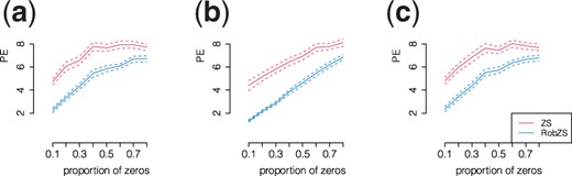
Prediction performance of the ZS (red) and RobZS (blue) estimators in scenario (B) by increasing the proportions of zeros in training and test data from 0.1 to 0.8 in steps of 0.1. Parameter configuration: (a) $n=50,p=30,\rho =0.2$⁠, (b) $n=100,p=200,\rho =0.2$⁠, (c) $n=100,p=1000,\rho =0.2$⁠. Shown are means (solid lines) plus/minus two standard errors averaged over 100 replications for each fixed proportions of zeros

As expected, the performance of both estimators linearly reduces as the proportion of zero counts in the covariates increases. However RobZS shows the best overall behavior even when the proportion of zero counts in the covariates is very high, as ZS is very much affected by outliers.

3.5 Simulations with increasing outlier proportion

The simulations in this section investigate the behavior of the estimators ZS and RobZS for increasing levels of contamination. We use contamination setting (C) and increase the outlier proportion from zero to 0.5 in steps of 0.02. In each step, 50 replications are carried out, and the means plus/minus two standard errors of the results are presented in Figure 2. The red lines are for ZS, the blue lines for RobZS. The simulations are conducted for the parameters n = 50, p = 30 and $\rho =0.2$⁠. The results basically reveal that the results for ZS get worse if the outlier proportion increases. Particularly, FN quickly increases to a value of about 2, and thus 2 out of 6 active variables are (on average) not identified. RobZS shows stable performance up to about 25% of contamination. This is explained by the trimming proportion of the procedure, which we set to 25% in all experiments. The evaluation with a 10% trimmed prediction error (upper right plot) is clearly not appropriate in a setting with high proportions of outliers. It is interesting that FN is very stable (up to about 20% contamination), and that FP decreases for an outlier proportion of up to 0.25. This means that the estimated regression parameters get sparser with higher contamination, and true noise variables are more accurately identified.

Fig. 2.

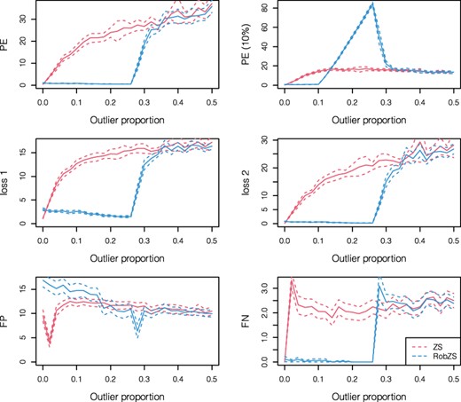
Performance of the ZS (red) and RobZS (blue) estimators by increasing the contamination level, using scenario (C). Here, n = 50, p = 30, $\rho =0.2$⁠; shown are means (solid lines) plus/minus two standard errors derived from 50 simulation replications at each step

Supplementary Section S2.3 of Supplementary Material also contains simulations studies which investigate the effect of varying sparsity. A general conclusion from these results is that less sparsity of the model reduces the advantage of the robust method. Or, in other words, RobZS has much better performance than ZS in presence of outliers, and if the true underlying model is very sparse.

Finally, a further simulation study is presented in Supplementary Section S2.4 of Supplementary Material which focuses on the use of the elastic-net penalty (both Ridge and Lasso). The comparison of ZS and RobZS reveals that RobZS tends to select on average a much smaller value for the tuning parameter α than ZS, which comes closer to a ridge penalty, and thus contains more variables in the model. Consequently, FP is generally higher for RobZS compared to ZS, but FN is considerably lower, even in the uncontaminated case. As expected, the prediction error is much smaller for the robust method in a contaminated scenario.

4 An application to human gut microbiome data

We applied the proposed RobZS model to a cross-sectional study of the association between diet and gut microbiome composition (Wu et al., 2011). In this study, fecal samples from 98 healthy individuals were collected and the microbiome dataset was produced by high-throughput sequencing of 16S rRNA, obtaining 6674 OTUs, the normalized counts of clustered sequences that depict bacteria types. We aim to predict caffeine intake, the continuous outcome of interest, based on the OTU abundances (Jaquet et al., 2009; Xiao et al., 2018). The microbiome dataset was previously preprocessed by Xiao et al. (2018) removing rare OTUs with prevalence less than 10%. Due to the high proportion of zero counts, we further retained OTUs that appeared in at least 25 samples, resulting in a matrix of dimension $n\times p=98\times 240$⁠. Additionally, we applied the quantile transformation to the caffeine intake to fulfill the underlying assumption of normality, as done in Xiao et al. (2018). Zero counts were replaced by the maximum rounding error of 0.5 to allow for the logarithmic transformation, which is a common practice in the context of analyzing microbiome data (Aitchison, 1986, Section 11.5). Note that in CODA analysis there are more sophisticated methods for zero replacement (Lubbe et al., 2021), but since this is not the focus of this paper, and because the proportion of zeros is also quite high with 49%, we stick to this simple replacement strategy.

For a fair investigation of the prediction performance of the four sparse estimators, a 5-fold CV procedure was repeated 50 times, resulting in 250 fitted models for each sparse regression method. This is a common way used in machine learning to reduce the error in the estimate of mean model performance. In the training set, the parameter selection follows the one described in the simulation section. Prediction error and trimmed prediction error were used to assess the prediction accuracy of the different methods. Note that instead of using a trimmed prediction error, one could also use other robust error measures if the outlier proportion is unknown, such as the robust τ scale estimator of Maronna and Zamar (2002).

Figure 3 shows the boxplots of the CV PEs (left) and the 10% trimmed CV PEs (right) over all replications for the estimators Lasso, ZeroSum, RobL, RobZS and SLTS. The estimators RobZS and SLTS show somewhat smaller prediction errors, and SLTS yields the smallest 10% trimmed PEs, at the cost of a larger variability. It can thus be assumed that there is a certain effect of outliers which influence the model estimation.

Fig. 3.

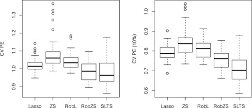
Analysis of gut microbiome data. Boxplots of CV PEs (left) and 10% trimmed CV PEs (right) over all replications for Lasso, ZeroSum, RobL, RobZS and SLTS

In order to investigate the impact of potential outliers in more detail, we can apply an outlier analysis on the scaled residuals. For each model fit within the CV scheme, the scale of the residuals for the CV training data can be estimated. This is done with the classical standard deviation; but for the robust fits we only include residuals from observations with weight 1 in the reweighting step, see Equation (9). Thus, outliers according to this weighting scheme will not affect the estimation of the residual scale. Then the residuals from the left-out folds are scaled with this estimator, and the CV PEs now include only the observations where the scaled residuals are within the interval $[-2.5,2.5]$⁠. The results are shown in the boxplots of the left panel of Figure 4, and in Figure 5. Figure 5 shows, for each model and over all CV replications, the mean of the scaled residuals for each observation. The residual scale was estimated from the model fit, and the scaled residuals are computed from the CV predictions. Since there are 50 CV replications, we can show the averages over 50 scaled residuals for each observation and for each estimator. The sorting of the observations on the horizontal axis is according to the RobZS mean. With the cutoff values ±2.5, shown as dashed lines, we see that SLTS identifies a huge amount of outliers when compared to the other estimators, i.e. more than 74% of the predicted values are flagged as anomalous, also their range is extremely large, suggesting that this model is inadequate for the example data we are dealing with. Consequently, the smaller CV PE without outliers for SLTS in the boxplot of Figure 4(left) is not comparable with the others as it is based only on few observations. RobZS instead identifies a more feasible number of outliers in the predictions, namely less than 30%.

Fig. 4.

Analysis of gut microbiome data. Left panel: Boxplot of CV PEs over all replications by Lasso, ZeroSum, RobL and RobZS. Only the observations whose corresponding scaled residuals are within the interval $[-2.5,2.5]$ were considered. Right panel: Fitted versus measured values of the transformed caffeine intake. The green points correspond to observations detected as outliers by the RobZS estimator

Fig. 5.

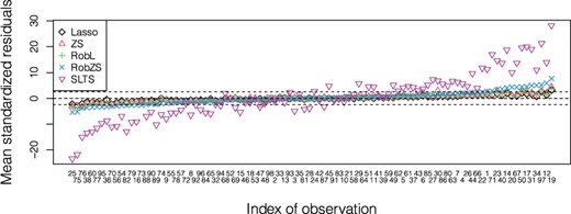
Analysis of gut microbiome data. Mean of the scaled CV prediction residuals for each observation. The sorting of the observations on the x-axis is according to the mean for RobZS

We can recognize that the RobZS estimator achieves the best performance, outperforming the other methods by a large margin. This is due to the robustness and precision of the RobZS estimator, which allows for a reliable outlier diagnostics for the predictions. This can also be seen in the right panel of Figure 4, where RobZS was simply applied to the complete dataset. The plot shows the measured versus fitted response variable, and the color corresponds to the weights from Equation (9). The green points correspond to observations detected as outliers by the RobZS estimator, namely data with binary weight w_i = 0. Based on the analysis in Figure 4 (right) we can also investigate which observations are potential (prediction) outliers.

The 250 models for each method, resulting from the described CV procedure, can be further analyzed for the variable selection performance. Figure 6 shows on the vertical axis the proportion of models containing at least the number of zeros in the regression parameter estimates indicated on the horizontal axis (in total 241 variables). A substantial proportion of models lead to a fully sparse solution; for RobL we obtain in about 60% of the models full or almost full sparsity. In contrast, SLTS yields much less sparsity, and the models are also very similar in terms of sparsity. RobZS seems to be best tunable, as this method leads to higher sparsity, but the proportion of fully sparse models is still the lowest.

Fig. 6.

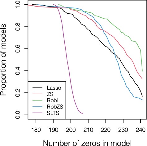
Analysis of gut microbiome data. Proportion of models (out of all 50 * 5) containing at least the number of zeros shown on the horizontal axis over all CV replications by Lasso, ZeroSum, RobL, RobZS and SLTS

Further investigations on application results are reported in Supplementary Section S3 of Supplementary Material.

5 Conclusions

We have proposed the robust ZeroSum (RobZS) regression estimator as a trimmed version of the ZeroSum (ZS) estimator, used in high-dimensional settings with compositional covariates. This model can be applied in microbiome analysis to identify bacterial taxa associated with a continuous response. Like in Lasso or elastic-net regression, the estimated regression coefficient vector is typically sparse. Additionally, however, the non-zero coefficients sum up to zero, and this constraint is appropriate for linear log-contrast models as they are used in the context of CODA analysis. In other words, the estimator is appropriately performing variable selection among compositional explanatory variables and allows for an interpretation of those selected compositional parts.

The estimation procedure of the RobZS estimator is based on an analogue of the fast-LTS algorithm in the context of robust regression. For the computation, a robust elastic-net regression procedure has been adapted and implemented. The conducted simulation studies reveal that the RobZS estimator has similar performance as the non-robust ZS estimator if there are no outliers, but in case of contamination (vertical outliers, leverage points) the robust version leads to a big advantage in terms of prediction error, precision of the estimated regression coefficients and ability to correctly identify the relevant variables (partly at the cost of a slightly increased false positive rate). Also when compared to other robust estimators such as sparse LTS (Alfons et al., 2013) or elastic-net LTS (Kurnaz et al., 2018), which however do not incorporate the compositional aspect of the data, RobZS is superior according to the evaluation measures in almost all settings. Simulations with zeros in the data, with varying sparsity and varying outlier proportions have further underlined the excellent performance of RobZS. The application to microbiome data has demonstrated that RobZS is capable to balance the sparsity of the solution with proper prediction accuracy. A further benefit is that outliers in the training data can be identified, but also for new data it is possible to indicate outlyingness, thus values of the explanatory variables or the response which do not match the training data.

In future work, this model will be extended to the generalized linear models framework for high-dimensional compositional covariates.

Acknowledgements

The authors wish to thank the Editor, the Associate Editor and the reviewers for their valuable comments and suggestions. They greatly acknowledge the DEMS Data Science Lab for supporting this work by providing computational resources.

Funding

This research was supported by local funds from University of Milano-Bicocca [FAR 2018 to G.S.M.].

Conflict of Interest: none declared.