Tumor heterogeneity assessed by sequencing and fluorescence in situ hybridization (FISH) data

Abstract

Motivation

Computational reconstruction of clonal evolution in cancers has become a crucial tool for understanding how tumors initiate and progress and how this process varies across patients. The field still struggles, however, with special challenges of applying phylogenetic methods to cancers, such as the prevalence and importance of copy number alteration (CNA) and structural variation events in tumor evolution, which are difficult to profile accurately by prevailing sequencing methods in such a way that subsequent reconstruction by phylogenetic inference algorithms is accurate.

Results

In this work, we develop computational methods to combine sequencing with multiplex interphase fluorescence in situ hybridization to exploit the complementary advantages of each technology in inferring accurate models of clonal CNA evolution accounting for both focal changes and aneuploidy at whole-genome scales. By integrating such information in an integer linear programming framework, we demonstrate on simulated data that incorporation of FISH data substantially improves accurate inference of focal CNA and ploidy changes in clonal evolution from deconvolving bulk sequence data. Analysis of real glioblastoma data for which FISH, bulk sequence and single cell sequence are all available confirms the power of FISH to enhance accurate reconstruction of clonal copy number evolution in conjunction with bulk and optionally single-cell sequence data.

Availability and implementation

Source code is available on Github at https://github.com/CMUSchwartzLab/FISH_deconvolution.

Supplementary information

Supplementary data are available at Bioinformatics online.

1 Introduction

Cancer progression has long been understood to be driven by clonal evolution (Nowell, 1976), but our understanding of the mechanisms and implications of that observation are currently undergoing a dramatic revision. This growing insight has been driven largely by two key innovations: the advance of high-throughput sequencing methods to characterize tumor genomics with ever-finer precision and accuracy (Mardis and Wilson, 2009) and the concurrent advance of computational methods to interpret those sequencing data to construct coherent accounts of how individual cancers or the space of all cancers collectively develop (Beerenwinkel et al., 2016). A crucial component of those latter advances has been the progress of tumor phylogenetics (Schwartz and Schäffer, 2017), i.e. constructing models of evolution in cancers from tumor genomic data.

Methods for clonal phylogenetics have attracted great interest in computational biology, concurrent with greater understanding of the complexity of tumor evolution mechanisms and the algorithmic challenges of reconstructing tumor phylogenies from available genomic data. A particular area of recent interest in this regard has been development of better methods for resolving evolution by copy number alterations (CNAs) and the structural variations (SVs) that may produce them. While the importance of CNAs and SVs in cancer has long been known (Zack et al., 2013) and some of the first methods for clonal lineage reconstruction focused on CNA-driven evolution (Pennington et al., 2007), much of the tumor phylogeny field has focused historically on single nucleotide variants (SNVs), with CNAs omitted (e.g. Yuan et al., 2015) or treated largely as a confounding factor for inferring SNV-driven evolution (e.g. El-Kebir et al., 2016a,b). Relatively few computational methods have been created to date for the purpose of inferring tumor evolution by CNAs, either singly (El-Kebir et al., 2016a,b, 2017; Schwarz et al., 2014; Tolliver et al., 2010) or jointly with SNVs (Jiang et al., 2016), and it is only recently that methods have begun to appear for capturing evolution by SVs more broadly (Eaton et al., 2018). Yet the biological evidence over the same time has strongly indicated that CNAs, and the SVs that may produce them, outperform SNVs and other focal changes in predicting treatment response (Shukla et al., 2020) and are likely the dominant mechanism by which tumors develop and functionally adapt to escape controls on cell growth (Zack et al., 2013).

CNA-driven evolution creates complications relative to SNV-driven evolution. In part, modeling CNAs is a challenge because it is less commonly studied in phylogenetics in general. Furthermore, CNAs create particular complications because they can occur recurrently in the same patient and on multiple scales with sometimes overlapping variations that can be difficult to resolve. CNAs are also particularly challenging for deconvolutional approaches to phylogenetics (Beerenwinkel et al., 2005), which computationally separate mixtures of clones from bulk sequence data and whose solutions are underdetermined without additional data or problem constraints. Using bulk data remains necessary because it is much more abundant than single-cell data. CNA methods have particular difficulty dealing with ploidy changes, particularly via whole-genome duplication (WGD), because ploidy is difficult to infer accurately from sequence data alone. While recent methods have shown it to be possible to perform accurate CNA construction using multi-region bulk sequencing (Zaccaria and Raphael, 2020) or single-cell sequencing (Zaccaria and Raphael, 2021), these methods require limiting assumptions, e.g. that WGD can occur only once in a tumor’s history. Furthermore, large cohorts with multi-region bulk or single-cell sequencing are still lacking and it remains an open question how best to perform large-scale tumor genomic studies that will be informative for clonal CNA evolution.

The problem of accurately reconstructing ploidy changes in tumor evolution is concerning, partly because WGD is now recognized as a statistical marker of aggressive cancers (Bielski et al., 2018; Koçak et al., 2020; Oltmann et al., 2018) but without a clear biological mechanism. Earlier models of WGD in tumor evolution, which proposed a single early WGD event as a prerequisite for tumorigenesis in chromosomally instable cancers (Dewhurst et al., 2014), are now known to be simplistic, as WGD is not necessary, but could occur multiple times in the same subclone or as separate events in different subclones during a cancer’s evolution (Oltmann et al., 2018). Rather, WGD can be seen to be one of many mutation types active to different degrees in different cancers, shaping the patient-specific risk of diverse progression processes (The ICGC/T CGAPan-Cancer Analysis of Whole Genomes Consortium, 2020).

The present work develops methods to improve resolution of CNA-driven evolution in cancers via a strategy of multi-omic data integration. Single-cell sequencing (Navin et al., 2011) has revolutionized tumor evolution studies and many methods are now available for deriving CNA-based tumor phylogenies from single-cell DNA sequence data, despite some continuing challenges of gathering and interpreting such data (Mallory et al., 2020; Zafar et al., 2018). Malikic et al. demonstrated that integrating bulk and single-cell sequencing data (Malikic et al., 2019) for improving SNV evolution models, a strategy we previously demonstrated successful for CNA-driven evolution as well (Lei et al., 2019). Here, we explore the potential of an additional form of data, multiplex interphase fluorescence in situ hybridization (miFISH), which can profile tumor evolution in single cells at small numbers of probes (Heselmeyer-Haddad et al., 2012) without normalization artifacts that make ploidy a challenge for purely sequence-based studies. While miFISH limits one to just a few copy number markers per cell, its easy scalability to large numbers of cells has made it a powerful tool for CNV tumor phylogenetics in its own right, especially when FISH probes are placed strategically at loci recurrently amplified in the tumor type of interest (Chowdhury et al., 2013; Pennington et al., 2007; Zhou et al., 2016). While individual miFISH probes in recurrently amplified regions may not give a reliable signal for WGD, prior work has shown that collective changes among just a few well-spaced miFISH probes provide sufficient signal to reliably distinguish focal CNAs from ploidy changes (Chowdhury et al., 2014, 2015; Gertz et al., 2016; Oltmann et al., 2018).

Here, we develop a new method for integrating bulk sequence with single-cell sequence (SCS) and/or miFISH in order to combine advantages of each technology for improved reconstruction of copy number evolution at the single cell level. We show with semi-simulated data that these two kinds of data each contribute in distinct and synergistic ways to more accurate inference of CNA-driven evolution, especially in aneuploid tumors, and demonstrate their practical value on a study of glioblastoma profiled by bulk, SCS and miFISH. The results support a model of WGD as an ongoing process of somatic evolution rather than a one-time event, potentially helping to explain why evidence of WGD is a risk factor for continuing tumor progression. Together, the work demonstrates the value of bringing miFISH or related methods for cytometric analysis into sequence-based tumor phylogeny studies if we are to accurately reconstruct mechanisms of CNA-driven evolution in cancers.

2 Materials and methods

2.1 Problem statement

While the mixed membership model in our previous work (Lei et al., 2019) is still suitable to describe our problem, the previous objective function is too simple for our new problem, since it does not include miFISH data. The miFISH data is relevant only at a few loci, but with an appropriate objective function, it allows us to estimate the genome-wide ploidy and thereby to inform the analysis of unnormalized (i.e. true) copy number at all loci. We therefore designed a new objective function for the problem intended to capture information from bulk copy numbers, miFISH copy numbers, single cell sequencing (SCS) data and phylogenetic constraints:

$$\begin{array}{c}\underset{\mathit{C},\mathit{F},\mathit{S},\mathit{P}}{\min }(||\mathit{B}-\mathit{CPF}|{|}_1+{\alpha }_f·\left|\right|\mathit{F}-\mathit{F}\prime |{|}_1\hfill \\ +{\alpha }_p·J(\mathit{S},\mathit{C},\mathit{C}\prime )+{\alpha }_c·\left|\right|{\mathit{X}}^T\mathit{CP}-\mathit{H}\prime |{|}_1)\hfill \end{array}$$

(1)

where the desired outputs are a matrix of inferred normalized copy numbers C of probes across the genome, a diagonal matrix P with the inferred ploidy divided by 2 for each in the diagonal, and an inferred clonal frequency matrix F. CP, then transforms the normalized cells with mean copy number two into unnormalized cells with putative absolute copy numbers. We refer to the outputs collectively as the inferred data.

We collectively call the algorithm’s inputs the observed data, which we distinguish from the ground truth, the hypothetical complete and noise-free data that are only knowable for simulated inputs. The potential inputs are $\mathit{F}\prime$⁠, a matrix of observed mixture fraction information derived from miFISH data by preclustering it to estimate clonal frequencies; $\mathit{C}\prime$⁠, an optional matrix of normalized copy numbers of observed SCS data that establish a reference set of single-cell clones; $\mathit{H}\prime$⁠, the observed copy numbers from miFISH data for the genomic regions covered by miFISH probes; and X, a 0-1 matrix in which the 1’s identify segments of the genome covered by each miFISH probe. ‘Covered’ means loosely that the segment includes or is close enough to the probe so that the correct unnormalized copy number in the segment is measured accurately by the miFISH probe, perhaps with a small amount of noise. S is a phylogeny inferred in the process of computing the objective function. $\left|\right|\mathit{B}-\mathit{CPF}|{|}_1$ is the deviation between observed and inferred mixed copy number in the bulk tumor. $\left|\right|\mathit{F}-\mathit{F}\prime |{|}_1$ describes the deviation between inferred mixture fraction F and observed mixture fraction $\mathit{F}\prime ,\hspace{0.17em}J(\mathit{S},\mathit{C},\mathit{C}\prime )$ is the cost of the phylogeny that is built on inferred cell clones C and observed single-cell clones $\mathit{C}\prime$ from a presumed non-cancerous diploid root; the definition of the tree and the cost-function can be found in Supplementary Section S1.3. We require C to be integral because homogeneous copy number is inherent to being a clone, but $\mathit{C}\prime$ need not be integral. X is a sparse matrix such that ${\mathit{X}}_{ij}=1$ if i is the index miFISH probe in the genomic position of single-cell data and $i=\mathit{Index}[j]$⁠, where each element in Index is the index of one miFISH probe on the genomic axis of the SCS data. The product ${\mathit{X}}^T\mathit{C}$ represents a subset of genomic position that contains only the copy number information for segments covered by miFISH probes and zeros elsewhere. Then $\left|\right|{\mathit{X}}^T\mathit{CP}-\mathit{H}\prime |{|}_1$ describes the deviation between inferred and observed copy number at loci where FISH probes are located.

Table 1 defines the three regularization parameters ${\alpha }_f$⁠, ${\alpha }_p$ and ${\alpha }_c$⁠, which we call ‘mixture fraction weight’, ‘phylogenetic weight’ and ‘copy number weight’ respectively. A full list of model variables is provided in Supplementary Table S1. We elaborate in the Supplementary Methods on specific constraints involving the terms of the objective function. All these terms are included in an integer linear programming (ILP) problem formulation that we solve through an iterative update algorithm making use of the Gurobi ILP solver.

Table 1.

Regularization parameters in the objective function

${\alpha }_f\in {\mathbb{R}}^{+}$	Weight of correspondence between inferred and observed miFISH mixture fractions, referred to as ‘mixture fraction weight’ for short
${\alpha }_p\in {\mathbb{R}}^{+}$	Weight of phylogenetic L1 model cost, referred to as ‘phylogenetic weight’ for short
${\alpha }_c\in {\mathbb{R}}^{+}$	Weight of correspondence between inferred and observed miFISH copy numbers, referred to as ‘copy number weight’ for short

Due to the complexity of the ILP, we sought a locally optimal solution to the constraints via a heuristic iterative coordinate descent optimization. The method iteratively solves for F, S, C and P in order, repeating these steps until the solution converges or a maximum number of iterations are reached. The ILP and associated optimization algorithm are described in Supplementary Methods Section S1.

2.2 Glioblastoma data

We apply the method to SCS and copy number data from two glioblastoma (GBM) patients (GBM07, GBM33), which were previously described in (Lei et al., 2019). We have samples from three tumor regions per patient and FISH data from cells in each region for eight gene locus probes: PDGFRA(4q), APC(5q), EGFR(7p), MET(7q), MYC(8q), CCND1(11q), CHEK1(11q) and ERG (21q), several of which were selected because they are sites of recurrent amplifications in GBM (The Cancer Genome Atlas Research Network, 2008). Indeed, both patients have copy numbers over 10 at several loci and patient GBM07 has an extreme amplification with copy numbers possibly over 50, at PDGFRA. We set an upper bound of 10 for normalized copy number, which was used directly for the SCS data. For miFISH data, which are not inherently normalized, we set an upper bound of 40, which allows for as many as 2 WGD on top of a normalized copy number of 10. Copy numbers greater than their respective uppper bound were set to their upper bound. The methods for designing FISH probes and counting FISH copy numbers have been previously described (Heselmeyer-Haddad et al., 2012, 2014; Oltmann et al., 2018).

2.3 Simulated data

We further rely on simulated data for validation due to the unavailability of real data with known ground truth. As in our prior work (Lei et al., 2019), we meet this need through semi-simulated data derived from observed GBM single-cell sequence data for which we artificially generate clonal mixtures of known composition and use these to generate synthetic bulk data and, in an extension of the prior work, synthetic miFISH data. We thus generate synthetic data for which true cell fractions and copy numbers are known, but with the goal of approximating as well as possible characteristics of the true GBM data described in Section 2.2. For this purpose, we generate six data structures per synthetic dataset:

1. $\tilde{\mathit{C}}$⁠: a matrix of normalized copy number profiles of all selected clones, used to compose bulk tumor data

2. $\widehat{\mathit{C}}$⁠: a matrix of normalized copy number profiles of major clones in $\tilde{\mathit{C}}$⁠, used to evaluate the performance

3. $\tilde{\mathit{P}}$⁠: a diagonal matrix of half ploidies of all selected clones

4. $\widehat{\mathit{P}}$⁠: a diagonal matrix of half ploidies of major clones

5. $\tilde{\mathit{F}}$⁠: a matrix of mixture fractions of all selected clones in each region

6. $\widehat{\mathit{F}}$⁠: a matrix of mixture fractions of major clones in each region

In the simulated data, we set the normalized maximum copy number to 10 as this is typically sufficient at most loci, except when there is an oncogenic amplification. Full details on the simulation protocol are provided in Supplementary Section S1.8.

3 Results

3.1 Evaluation on simulated data

3.1.1 No ploidy change

We first evaluated the method on simulated data with no ploidy changes, i.e. all diploid data, to provide a basis for comparison with pure deconvolution and with our previous work (Lei et al., 2019), which did not explicitly model ploidy. Each test made use of bulk data and the $\left|\right|\mathit{B}-\mathit{CPF}\left|\right|$ deconvolution objective, but we varied tests by whether or not we used each of the other objective terms—$\left|\right|\mathit{F}-\mathit{F}\prime \left|\right|,\hspace{0.17em}J(\mathit{S},\mathit{C},\mathit{C}\prime )$ and $\left|\right|{\mathit{X}}^{\mathit{T}}\mathit{CP}-\mathit{H}\prime \left|\right|$—to determine how they contribute individually or in combination to overall accuracy. As shown in Figure 1a, solving the pure deconvolution problem alone yielded poor average accuracy (Fig. 1a, [i], red bar), although the results improved substantially when we used true SCS data to initialize the method (Supplementary Fig. S7). This observation is consistent with our prior work (Lei et al., 2019), although the absolute accuracy of these two variants is worse than in our previous work. The difference is due to a change in initialization conditions as explained in Supplementary Section S2.4 and Supplementary Figures S6 and S7.

Fig. 1.

Average accuracy and RMSD of the deconvolution without ploidy change (n = 10). (a) Without noise. (b) With 10% noise. In each subplot of [i]–[v], the bar plot shows the average error (1 - accuracy) of copy number, average RMSD of copy number, average RMSD of mixture fraction, average RMSD of ploidy and average RMSD of unnormalized copy number. Each bar with a different color represents a deconvolution model with different parameter values. The number in the first row under the bar indicates a set of parameter values, the number in the second row under the bar indicates the mean for those parameter values, and the whiskers show the standard deviation. The legend at the bottom right of (a) shows the combination of parameter values corresponding to each bar of each subplot, numbered in the same order as they appear in the subplot. Each row of three numbers provides the value of mixture fraction weight α_f, phylogenetic weight ${\alpha }_p$ and copy number weight ${\alpha }_c$⁠, which are regularization terms for $\left|\right|\mathit{F}-\mathit{F}\prime \left|\right|,\hspace{0.17em}J(\mathit{S},\mathit{C},\mathit{C}\prime )$ and $\left|\right|{\mathit{X}}^{\mathit{T}}\mathit{CP}-\mathit{H}\prime \left|\right|$⁠, respectively. 0.0 means the corresponding term was not included in the model. Statistically significant improvements from incorporating FISH data were assessed by paired sample t-test, comparing green (2), pink (3) and gray (4) bars to the NULL model [red bar (1)] and orange (6), cyan (7), coral (8) bars to the single-cell only model [blue bar (5)] (n.s.: not significant, *: $0.05<$P-value$\le 0.1$⁠, **: $0.01<$P-value$\le 0.05$⁠, ***: P-value$\le 0.01$⁠)

Including the term $J(\mathit{S},\mathit{C},\mathit{C}\prime )$ had a large positive effect on the copy number inference but little impact on the mixture fraction inference (Fig. 1a, [iii], blue bar). However, adding $\left|\right|\mathit{F}-\mathit{F}\prime \left|\right|$ to the objective function, and thus using miFISH to correct inferred clonal mixture fractions, substantially improved the inference accuracy for both mixture fractions and copy numbers (Fig.1a, [i] and [iii], green bar). We further found that the combination of the two terms above (mixture fraction weight ${\alpha }_f=0.2$⁠, phylogenetic weight ${\alpha }_p=0.2$⁠, copy number weight ${\alpha }_c=0.0$⁠) further improved the performance in both copy number inference and mixture fraction inference (Fig.1a, [i] and [iii], cyan bar), showing these two components act in a complementary fashion.

The inclusion of $\left|\right|{\mathit{X}}^{\mathit{T}}\mathit{CP}-\mathit{H}\prime \left|\right|$ alone (mixture fraction weight ${\alpha }_f=0.0$⁠, phylogenetic weight ${\alpha }_p=0.0$⁠, copy number weight ${\alpha }_c=0.2$⁠), with $\left|\right|\mathit{F}-\mathit{F}\prime \left|\right|$  $({\alpha }_f=0.2,{\alpha }_p=0.0,{\alpha }_c=0.2)$⁠, or with $J(\mathit{S},\mathit{C},\mathit{C}\prime )$  $({\alpha }_f=0.0,{\alpha }_p=0.2,{\alpha }_c=0.2)$ yields further improvement (Fig. 1a, [i] and [ii], violet, gray and orange bars) in copy number and mixture fraction inference. Including both $\left|\right|{\mathit{X}}^{\mathit{T}}\mathit{CP}-\mathit{H}\prime \left|\right|$ and $J(\mathit{S},\mathit{C},\mathit{C}\prime )$  $({\alpha }_f=0.0,{\alpha }_p=0.2,{\alpha }_c=0.2)$ also substantially improved mixture fraction inference (Fig. 1a, [iii], orange bar) compared to $J(\mathit{S},\mathit{C},\mathit{C}\prime )$  $({\alpha }_f=0.0,{\alpha }_p=0.2,{\alpha }_c=0.0)$⁠. These results show that the improvements from each objective component and from miFISH and SCS data are cumulative. Furthermore, the model with all three weights greater than 0 (⁠${\alpha }_f=0.2,\hspace{0.17em}{\alpha }_p=0.2,\hspace{0.17em}{\alpha }_c=0.2$⁠) yielded the best results for mixture fraction inference and both normalized and unnormalized copy number inference (Fig. 1a, [i]–[iii] and [v], coral bars).

We then examined the robustness of the algorithm to noise. As described in Section 2.3, we introduced 10% noise to the reference data. The results were similar to those without noise and yielded qualitatively similar conclusions. Although the model loses some accuracy, it is fairly robust to moderate noise with the current parameters (Fig. 1b).

3.1.2 With ploidy change

We next examined performance when samples can have variable ploidies. We observed overall lower accuracy of inference across tests when ploidy was variable, although a qualitatively similar profile to the diploid case in Section 3.1.1 in how different combinations of objective function terms contributed to accuracy. Pure deconvolution without any single-cell information performed worse when the ground truth data exhibit variable ploidy (Fig. 2a, [i], red bar). Combining the $J(\mathit{S},\mathit{C},\mathit{C}\prime )$ and $\left|\right|{\mathit{X}}^{\mathit{T}}\mathit{CP}-\mathit{H}\prime \left|\right|$ terms, i.e. $({\alpha }_f=0.0,{\alpha }_p=0.2,{\alpha }_c=0.2)$⁠, yielded more improvement when ploidy is variable (Fig. 2a, [i], blue and orange bars), though the standard error increased. Furthermore, the model with all three terms yielded the best accuracy to a significant degree by all measures considered (Fig. 2a coral bar), showing that each term contributed synergistically to overall accuracy when ploidy was variable.

Fig. 2.

Average accuracy and RMSD of the deconvolution with ploidy change (n = 10). (a) Without noise. (b) With 10% noise. In each subplot of [i]–[v], the bar plot shows the average error (1 - accuracy) of copy number, average RMSD of copy number, average RMSD of mixture fraction, average RMSD of ploidy and average RMSD of unnormalized copy number. Each bar with a different color represents a deconvolution model with different parameter values. The number in the first row under the bar indicates a set of parameter values, the number in the second row under the bar indicates the mean for those parameter values, and the whiskers show the standard deviation. The legend at the bottom right of (a) shows the combination of parameter values corresponding to each bar of each subplot, numbered in the same order as they appear in the subplot. Each row of three numbers provides the value of mixture fraction weight α_f, phylogenetic weight ${\alpha }_p$ and copy number weight ${\alpha }_c$⁠, which are regularization terms for $\left|\right|\mathit{F}-\mathit{F}\prime \left|\right|,\hspace{0.17em}J(\mathit{S},\mathit{C},\mathit{C}\prime )$ and $\left|\right|{\mathit{X}}^{\mathit{T}}\mathit{CP}-\mathit{H}\prime \left|\right|$⁠, respectively. 0.0 means the corresponding term was not included in the model. Statistically significant improvements from incorporating FISH data were assessed by paired sample t-test, comparing green (2), pink (3) and gray (4) bars to the NULL model [red bar (1)] and orange (6), cyan (7), coral (8) bars to the single-cell only model [blue bar (5)] (n.s.: not significant, *: $0.05<$P-value$\le 0.1$⁠, **: $0.01<$P-value$\le 0.05$⁠, ***: P-value$\le 0.01$⁠)

When we introduced 10% noise to the data, the conclusions were qualitatively similar (Fig. 2b). The complete model $({\alpha }_f=0.2,{\alpha }_p=0.2,{\alpha }_c=0.2)$ again performed the best by all evaluation measurements.

3.1.3 Phylogenetic output

Finally, we compared the phylogenetic outputs of the current models. Since the phylogenetic results from the experiments with no ploidy change were trivial (all the ploidies were around 2), we considered only the models with ploidy changes. We chose the case with the highest overall accuracy of copy number as representative and plotted the phylogenetic trees of three different models that introduce the $J(\mathit{S},\mathit{C},\mathit{C}\prime )$ term, $J(\mathit{S},\mathit{C},\mathit{C}\prime )$ and $\left|\right|{\mathit{X}}^{\mathit{T}}\mathit{CP}-\mathit{H}\prime \left|\right|$ terms, and all three terms, respectively (Fig. 3). In each case, nodes 0–5 represent the inferred cell components, nodes 6–11 represent the reference cells we observed from the available SCS data, and node 12 represents the assumed diploid root. In each node, we use the notation $\mathit{NodeIdx};P\mathit{loidy}$ to denote the index of a cell component (cell subclone) and its corresponding ploidy. For example, 12; 2 represents the 12th cell component (root) and the ploidy of this cell component is 2.

Fig. 3.

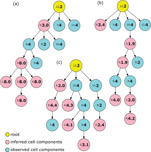
Phylogenetic trees for observed and inferred cell components on simulated data. The yellow node represents a diploid root cell, the pink nodes are inferred cell components and the light blue nodes are observed cell components. The number pair inside each node provides $\mathit{NodeIndex};\mathit{Ploidy}$⁠. (a) is the result from the model only including the $J(\mathit{S},\mathit{C},\mathit{C}\prime )$ term, (b) from the model including $J(\mathit{S},\mathit{C},\mathit{C}\prime )$ and $\left|\right|{\mathit{X}}^{\mathit{T}}\mathit{CP}-\mathit{H}\prime \left|\right|$ and (c) from the complete model

When we included only $J(\mathit{S},\mathit{C},\mathit{C}\prime )$  $({\alpha }_f=0.0,{\alpha }_p=0.2,{\alpha }_c=0.0)$⁠, most of the inferred cell components yielded unrealistically large copy numbers of 8.0, and the observed and inferred cell components tended to cluster together (Fig. 3a). This may be due to a model tendency to enlarge the ploidy of each inferred cell component to compensate for the deviation between copy number vectors in observed cell components.

When we added the $\left|\right|{\mathit{X}}^{\mathit{T}}\mathit{CP}-\mathit{H}\prime \left|\right|$ term to update the model $({\alpha }_f=0.0,{\alpha }_p=0.2,{\alpha }_c=0.2)$⁠, the ploidy of inferred cell component became more realistic, and the inferred and observed cell components showed less obvious partitioning (Fig. 3b). We observed that the diploid cell components tended to cluster together (e.g. node 2 → node 8) and tetraploid components tended to cluster together (e.g. node 6 → node 3). We inferred potential WGD events between diploid and tetraploid cell components (e.g. node 5 → node 6). This again suggests that the ploidy information from FISH data helps to correct for inferences difficult to make from sequence alone and restores a meaningful phylogenetic structure with ploidy inference among the cell components. Introducing $\left|\right|\mathit{F}-\mathit{F}\prime \left|\right|$ and $J(\mathit{S},\mathit{C},\mathit{C}\prime )$ together yielded a similar pattern (data not shown), suggesting as we might expect that more accurate clonal frequencies can also correct for the ambiguity in inference of F and C simultaneously that makes the pure copy number deconvolution problem challenging. When we used the complete model $({\alpha }_f=0.2,{\alpha }_p=0.2,{\alpha }_c=0.2)$⁠, the phylogenetic tree became more branched, and the diploid and tetraploid cell components were perfectly divided into different branches (node 0 → node 7, root → node 10 and root → node 11). Also, the potential WGD events were inferred to happen earlier in the progression (root → node 10 and node 5 → node 0). Furthermore, unlike in the previous trees (e.g. node 10 → node 2 in Fig. 3b), we see no biologically implausible reversion of WGD events in which ploidy is exactly halved. In addition, although most simulated ploidies in the representative data are tetraploidy, the model is still able to infer a triploidy case (node 9 → node 3 in Fig. 3c). All these observations again confirmed that the complete model $({\alpha }_f=0.2,{\alpha }_p=0.2,{\alpha }_c=0.2)$ not only reconstructed the heterogeneity with best accuracy and performance but also provided the most plausible phylogenetic structure for all the cell components.

Supplementary Sections S1.9, S2.7 and S2.1 further demonstrate that FISH constraints improve phylogeny inference accuracy, using fully simulated data with known ground truth trees and minimum evolutionary distance as a proxy for correctness on semi-simulated data. Supplementary Section S2.8 further compares our method to MEDALT (Wang et al., 2021), a recently published method for inferring phylogenetic trees from single-cell copy numbers alone, suggesting that the addition of bulk data and FISH data yields large improvements in the accuracy of phylogenetic trees under conditions of limited single-cell data.

3.2 Real GBM data

Finally, we applied the complete model with predefined parameters in which the mixture fraction weight, phylogenetic weight and copy number weight are all set to 0.2 on the real glioblastoma cases GBM07 and GBM33. The data include unnormalized copy numbers of bulk sequencing, normalized copy numbers of single-cell sequencing, and unnormalized copy numbers of miFISH. As in our other tests, normalized copy numbers from single-cell sequencing were restricted to be at most 10. We put a corresponding restriction of 40 on unnormalized miFISH copy numbers, because very high copy numbers are difficult to count accurately in miFISH and because it is unrealistic to model amplification of copy numbers above 40 by changes in chromosome number. We used k-median clustering of SCS and miFISH data to choose k = 6 clusters as the reference cells and reference FISH. The copy numbers of bulk samples, profiles of copy number (SCS and FISH) of the cluster centers and profiles of ploidy (FISH) of the cluster centers are the inputs to our the model. We ran the method ten times per patient with different randomly selected real reference data.

Figure 4 shows typical representative solutions for each case. (For clarity, an expanded version of the figure is included in Supplementary Fig. S9a–d), along with plots of the copy number across the genomic axis for each inferred cell component (Supplementary Fig. S9e and f). Since in the real SCS samples, we do not have the true ploidy information, we use ‘?’ to label the ploidy in observed cell components (Fig. 4b and d). We first focus on the GBM07 case (Fig. 4a and b and Supplementary Fig. S9e). We observed a pattern of focal CNAs consistent with those described previously in (Lei et al., 2019). Previous work showed that glioblastomas tend to display at least some chromosome-scale CNAs, such as chromosome 7 gain, chromosome 9p loss and chromosome 10 loss (Abou-El-Ardat et al., 2017; Crespo et al., 2011; Davis et al., 2016). The inferred cell components here all showed gain of chromosome 7 and loss of chromosome arm 9p, suggesting these are early events in the tumor’s evolution. One of the inferred components also showed loss of chromosome 10 (Supplementary Fig. S9e). In addition to the frequent focal aberrations, other chromosomes also displayed evidence of whole-chromosome gains (e.g. chromosome 8, 9 and 19) and losses (e.g. chromosome 8, 11). There is, however, some notable clonal heterogeneity, similar to inter-tumor heterogeneity observed in systematic studies of GBM (Crespo et al., 2011; McNulty et al., 2019).

Fig. 4.

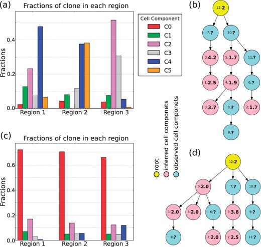
Application on real GBM07 (a, b) and GBM33 (c, d) cases. (a), (c) The corresponding mixture fraction of each inferred cell component. (b), (d) The phylogenetic relationship among the inferred cell components (pink) and observed cell components (light blue)

Several studies have shown that WGD occurs in about 25% of glioblamstoma cases (Bielski et al., 2018; Boisselier et al., 2018; Carter et al., 2012) and have suggested that it is an early event when it occurs. Our model for the GMB07 tumor supports an inference of two distinct WGD events on distinct cell lineages: an early WGD in the transition from components 12 through 7 to 0 and a late WGD event in the transition from component 4 to 3. This inference that there are multiple WGD events depends on having both sequence data supporting the tree topology and FISH data supporting the specific ploidy changes and therefore supports the value of the miFISH analysis in providing more direct measurements of ploidy and allowing sampling of larger numbers of cells, and thus better detection of rarer clones. Although we do not have information about the ploidy for the observed cell components, we may infer them based on the fact that the components with similar ploidy tend to occur in the same branches on the tree (Fig. 3c). A manual maximum parsimony imputation of WGD events suggests that all other observed components are most likely diploid with the possible exception of component 7, for which diploidy and tetraploidy are equally plausible.

Prior pan-cancer studies have suggested that WGD often touches off a cascade of more localized CNA losses, with particular marked chromosome losses (Zack et al., 2013) leading to a pseudotriploid form observed in past miFISH study of WGD-prone tumors (Oltmann et al., 2018). Conversion from tetraploidy to pseudotriploidy is evident in the transition from component 0 to 1. Further, focal CNA is evident in all of the inferred components but particularly pronounced for the two tetraploid components 0 and 3 and the pseudotriploid component 1 (Supplementary Fig. S9e).

The mixture fractions of the inferred clones provide additional insight into likely GBM progression. Components 2 and 4 (pink and blue bars in Fig. 4a) have relatively large proportions in two of the three regions, suggesting that their common features might be close to an ancestral population from which the tumor as a whole arose. That is consistent with the finding that chromosome 7 gain and chromosome 9p loss found in this component are early CNA events in the tumor and perhaps key drivers of tumorigenesis. Noticeable proportions of the non-diploid components 1 and 3, inferred to derive from distinct WGD events, are found in at least in one region (green and gray bars in Fig. 4a) but with sizable differences by region. This inference is again consistent with the idea that the tumor has been shaped by multiple distinct WGD events, with different regions of the tumor dominated by cell lineages tracing to different WGD events.

Figure 4c and d and Supplementary Fig. S9f show the results for the GBM33 case. Although we observed some similar events to GBM07, such as (partial) gain on chromosome 7 and loss on chromosome 9p and partial loss on chromosome 10, the global pattern of CNAs is quite different. First, GBM33 exhibits a pattern more dominated by focal CNA rather than chromosome-scale changes. Second, GBM33 shows less extreme changes at sites of high amplification than does GBM07 even where they amplify common loci (e.g. large copy numbers in GBM07 on chromosome 4, Supplementary Fig. S9e and f). Third, there appears to be just a single tetraploid inferred clone, clone 3, with pseudotriploid clone 2 descended from it (Fig. 4d). Maximum parsimony would suggest that the observed single cells are likely largely diploid, with the exception of clone 7 for which the assignment to diploid or tetraploid is ambiguous.

Fourth, GBM33 overall shows less pronounced clonal heterogeneity, with the single diploid clone 0 dominant in all three tumor regions. Notably, the tetraploid clone is inferred to be fairly rare, with the pseudotriploid clone slightly more common but still minor. The quite different reconstruction in the case of GBM33 versus GBM07 indicates that the method is sensitive to variations in profiles of CNA tumor-to-tumor.

4 Discussion

We have extended tumor phylogeny methods to incorporate copy number measurements by DNA-FISH, in addition to bulk and single-cell sequence data, as a source of more precise measurements of tumor ploidy and clonal frequencies. The results show that each source of data contributes separately to a more accurate picture of copy number evolution in cancers, with the combination of all three data types yielding improved accuracy in resolution of whole-genome copy number profiles. We demonstrated by application to two glioblastoma cases that the new methods can provide novel insight into the role of copy number evolution in cancers, supporting a model of WGD as an ongoing process of somatic evolution rather than a single event in early tumor evolution, which may better explain the importance of WGD as a marker for risk of future progression. The results suggest the value of supplementing sequence data with additional data sources such as miFISH in accurately reconstructing evolution by CNA mechanisms in tumors exhibiting chromosome instability.

Our work suggests a number of avenues for further research. One limitation of our method is that few tumors currently are studied by the combinations of technologies examined here. We suggest that it will be enlightening to conduct further studies where sequence is paired with miFISH, or perhaps alternative methods providing similar ability to estimate ploidy and/or clonal frequency, particularly for understanding evolution in cancer types prone to chromosome instability and aneuploidy. Second, the present work, like our prior work (Lei et al., 2019), suggests the value of an accurate single-cell phylogenetic model in improving deconvolution. Accurately reconstructing evolutionary trees in copy number space, even with known single-cell data, remains a challenging problem. While there is prior theory for reconstructing copy number evolution (Chowdhury et al., 2015; El-Kebir et al., 2017), no models are comprehensive for all known mechanisms of CNA evolution and developing comprehensive models and the algorithmic framework to make them scalable to large single-cell, whole genome data remains a challenge. It would also be valuable to extend the method to encompass automated parameter selection. There are also many other alternative technologies that might be incorporated into the mix of multi-omic data to improve phylogeny inference (e.g. long read or linked read sequencing, single-cell RNA-seq and bulk RNA-seq) that have been considered in other work (e.g. Tao et al., 2019) and might provide other synergistic advantages for the present problem. In principle, it would be especially attractive to include single-cell RNA-seq to evaluate the effects on gene expression associated with changes in single-cell DNA-seq, but the high dropout rate in single-cell sequencing would make this analysis complex in practice, since RNA-seq dropout cannot be as easily managed by averaging over larger regions as it is with CNA analysis from DNA-seq. In addition, there is likely room for improvement in better solving the central optimization problem of our work. Additional results (see Supplementary Results) show that increasing the number of rounds of optimization from 10 to 100 frequently leads to improvement in the objective function, although this improvement translates into negligible change in mean accuracy and RMSD measures. This observation suggests potential for improvement in both the definition of the objective function, to better match true solution quality, and in the algorithms, for efficiently solving for the objective.

Funding

This research was supported in part by the Intramural Research Program of the National Institutes of Health, National Library of Medicine and both Center for Cancer Research and Division of Cancer Epidemiology and Genetics within the National Cancer Institute. This research was supported in part by the Exploration Program of the Shenzhen Science and Technology Innovation Committee [JCYJ20170303151334808]. Portions of this work was funded by US NIH award R21CA216452 and Pennsylvania Department of Health awards [4100070287 and FP00003273]. Research reported in this publication was supported by the National Human Genome Research Institute of the National Institutes of Health under Award Number [R01HG010589]. The content is solely the responsibility of the authors and does not necessarily represent the official views of the National Institutes of Health. The Pennsylvania Department of Health specifically disclaims responsibility for any analyses, interpretations or conclusions. This work utilized the computational resources of the NIH HPC Biowulf cluster (http://hpc.nih.gov) to compare performances of the optimization packages Gurobi (www.gurobi.com) and SCIP (scip.zib.de).

Conflict of Interest: none declared.

Data availability

Simulated data and additional results are provided with the source code at https://github.com/CMUSchwartzLab/FISH_deconvolution. Human subjects data from the Beijing Genomics Institute (BGI) used for validation for this study are currently prohibited from public release.

Author notes

The authors wish it to be known that, in their opinion, the first two authors should be regarded as Joint First Authors.