Cancer subtype identification by consensus guided graph autoencoders

Abstract

Motivation

Cancer subtype identification aims to divide cancer patients into subgroups with distinct clinical phenotypes and facilitate the development for subgroup specific therapies. The massive amount of multi-omics datasets accumulated in the public databases have provided unprecedented opportunities to fulfill this task. As a result, great computational efforts have been made to accurately identify cancer subtypes via integrative analysis of these multi-omics datasets.

Results

In this article, we propose a Consensus Guided Graph Autoencoder (CGGA) to effectively identify cancer subtypes. First, we learn for each omic a new feature matrix by using graph autoencoders, where both structure information and node features can be effectively incorporated during the learning process. Second, we learn a set of omic-specific similarity matrices together with a consensus matrix based on the features obtained in the first step. The learned omic-specific similarity matrices are then fed back to the graph autoencoders to guide the feature learning. By iterating the two steps above, our method obtains a final consensus similarity matrix for cancer subtyping. To comprehensively evaluate the prediction performance of our method, we compare CGGA with several approaches ranging from general-purpose multi-view clustering algorithms to multi-omics-specific integrative methods. The experimental results on both generic datasets and cancer datasets confirm the superiority of our method. Moreover, we validate the effectiveness of our method in leveraging multi-omics datasets to identify cancer subtypes. In addition, we investigate the clinical implications of the obtained clusters for glioblastoma and provide new insights into the treatment for patients with different subtypes.

Availabilityand implementation

The source code of our method is freely available at https://github.com/alcs417/CGGA.

Supplementary information

Supplementary data are available at Bioinformatics online.

1 Introduction

Cancer is a type of disease that involves abnormal cell growth and can potentially invade or spread to other organisms of the body. As one of the leading causes of death worldwide, its heterogeneity is considered as the major problem limiting the efficacy of targeted therapies and compromising treatment outcomes (Janku, 2014). Cancer subtype identification aims to divide patients into groups with similar clinical phenotypes or molecular profiles, thus facilitating the prognosis and personalized treatment prediction in cancer (Huang et al., 2019; Kuijjer et al., 2018). For instance, it is now well-recognized that there are four main subtypes in breast cancer, i.e. Luminal A, Luminal B, Basal and HER2, each of which has distinct morphologies and responds differently to both targeted and chemotherapeutic agents (Dai et al., 2015; Salvadores et al., 2020).

With the rapid development of high-throughput sequencing techniques, large-scale projects such as The Cancer Genome Atlas (TCGA) have accumulated massive amount of diverse omics data for various cancer types (Cancer Genome Atlas Research Network et al., 2013; Speicher and Pfeifer, 2015). As a result, great computational efforts have been made to accurately identify cancer subtypes by integrative analysis of these multi-omics data (Chen et al., 2019; Rappoport and Shamir, 2018; Tepeli et al., 2020). Since the subtypes of most cancer samples are unclear, clustering has been widely used for cancer subtyping (Xu et al., 2019). Early methods generally make predictions by employing only one type of multi-omics data or directly concatenating all omics data followed by traditional single-omic clustering algorithms (e.g. k-means). However, this approach cannot fully exploit the underlying connections among different types of omics data and might lead to inaccurate results. Moreover, the simple concatenation strategy will also increase the data dimension and thus reduce the computational efficiency.

Multi-view clustering has recently become a hot topic in the field of machine learning(Nie et al., 2018; Xu et al., 2016). The goal of multi-view clustering is to make use of heterogeneous information from different views to provide a comprehensive result (Tang et al., 2019; Wang et al., 2020a,b). To take advantage of multi-omics datasets and understand sample characteristics from a more comprehensive perspective, many methods based on multi-view clustering have been developed to uncover potential subtypes in cancers (Jiang et al., 2019a,b; Li et al., 2018; Nguyen and Wang, 2020). According to the underlying model assumptions, existing cancer subtyping approaches can be roughly divided into several categories. Algorithms in the first category mainly utilize statistical models to fulfill the task (Vaske et al., 2010). One of the representative works is iCluster (Shen et al., 2009), a joint latent variable model for integrative clustering which simultaneously incorporates flexible modeling of the associations between different data types and reduces the dimensionality of the datasets. Although powerful, this method has a high computational cost with respect to the number of features and is relatively sensitive to the feature preselection step. LRACluster is an integrative probabilistic model to fast find the shared principal subspace across multiple data types by using low-rank approximation. Specifically, samples were clustered in a reduced low-dimensional subspace to identify the molecular subtypes (Wu et al., 2015). Another group of identification methods are generally based on multi-view similarity learning and different integration strategies are adopted to obtain the cluster labels for patients. Wang et al. first computed a sample-similarity network for each data type and then fused these networks into a single similarity network non-linearly (Wang et al., 2014). Finally, spectral clustering was applied on the obtained similarity network to get the results for cancer subtyping. In this way, the complementarity in the data were well explored. Cai et al. tried to find a consensus kernel matrix from a set of kernel matrices constructed for each data type. To solve the inconsistency among different views, they decomposed each kernel matrix into a consensus part together with a disagreement part and further defined a consensus score to measure the consistency (Cai and Li, 2017). In addition to the methods mentioned above, other representative subtyping methods include PINS (Nguyen et al., 2017), iNMF (Yang and Michailidis, 2016), JIVE (O'Connell and Lock, 2016) and so on. PINS discovered meaningful cancer subtypes based on perturbation clustering. The main idea is to repeatedly perturb the data by adding Gaussian noise and find the sample partitions that are least affected by the perturbations. iNMF is based on joint non-negative matrix factorization and can leverage the advantage of multiple data sources to gain robustness to heterogeneous perturbations. JIVE extends the principal components analysis to multi-source scenario and finds the joint structure by quantifying the amount of shared variation between data sources.

Although great computational efforts have been made in the past decade, it still remains a challenging task to discover biologically meaningful subgroups in cancer samples. Specifically, most of the existing methods only consider either the feature content or the graph structure of samples during the identification process, which cannot fully exploit the clustering information hidden in the samples. Besides, the graph structures used by many alternatives are constructed directly from the feature contents and are fixed throughout the optimization process, which might lead to sub-optimal performances due to the existence of noise in omics data and impedes the consistency sharing among multiple views. To solve these issues, in this article, we propose a Consensus Guided Graph Autoencoder (CGGA) to effectively identify cancer subtypes. Our method mainly consists of two steps. First, we learn for each omic a new feature matrix by using graph autoencoders, where both the structure information and node features are simultaneously considered during the learning process. Second, we learn a set of omic-specific similarity matrices as well as a consensus matrix based on the features obtained in the first step. Then, the learned omic-specific similarity matrices are fed back to the graph autoencoders to guide the feature learning. By iterating the two steps above, our method obtains a final consensus similarity matrix for cancer subtyping. Experimental results on both generic machine learning datasets and cancer datasets confirm the effectiveness of our method. Moreover, the survival analysis as well as the enrichment analysis based on the subgroups uncovered in glioblastoma provides new insights into the importance of cancer subtype identification.

2 Materials and methods

As aforementioned, our proposed algorithm consists of two parts, i.e. latent representation learning by GAEs and adaptive similarity graph learning based on the obtained representations (Fig. 1). The two parts are enhanced with each other in an iterative manner. We will first summarize the notations used in our work and then give details of each part in the following subsections.

Fig. 1.

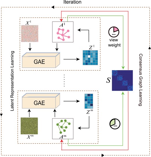
An overall workflow of the proposed method. It iterates between two parts, i.e. latent representation learning and consensus graph learning, until convergence

2.1 Basic notations

Throughout the article, we use italic uppercase letters to denote matrices. Given a matrix M, its jth column and (i, j)th element are denoted as m_j and m_ij, respectively. M^T, Tr(M) and ${‖\mathrm{M}‖}_{\mathrm{F}}\mathrm{\hspace{0.17em}}$denote the transpose, the trace and the Frobenius norm of M, respectively. 1 is a column vector with all ones and I is the identity matrix.

2.2 Graph autoencoders and its optimization

2.2.1 Graph convolutional networks

Graph Convolutional Networks(GCNs) are an efficient variant of Convolutional Neural Networks (CNNs) on graphs and have been widely used in various semi-supervised learning tasks (Kipf and Welling, 2016a,b; Wu et al., 2019). Given an attributed graph G(X, A), where $X=[x_1;x_2;\dots ;x_n]\in {\mathbb{R}}^{n\times d}$ is the node feature matrix and $A\in {\mathbb{R}}^{n\times n}$ encodes the similarities between each pair of nodes, a GCN aims to learn a latent representation $Z=[z_1;z_2;\dots ;z_n]\in {\mathbb{R}}^{n\times p}(p\le d)$ by simultaneously considering both the node features X and the graph structure A (Jiang et al., 2019a,b). Specifically, the layer-wise propagation rule of GCNs is:

$$Z^{l+1}=\sigma (\tilde{A}{Z}^l{W}^l),$$

(1)

where $Z^l\in {\mathbb{R}}^{n\times d_l}$ is the input feature matrix at the lth layer and Z⁰=X. $W^l\in {\mathbb{R}}^{d_l\times d_{l+1}}$ is a trainable weight matrix at the lth layer. $\tilde{A}={\tilde{D}}^{-\frac{1}{2}}(A+I_n){\tilde{D}}^{-\frac{1}{2}}$ and $\tilde{D}$ is a diagonal matrix with its ith element defined as ${\tilde{D}}_{ii}={\sum }_k{(A+I_n)}_{ik}$⁠. σ(˙) is an activation function such as ReLU. Based on Equation (1), a typical GCN can be easily constructed with predefined number of layers and the feature dimensions at each layer.

2.2.2 Graph AutoEncoders

Graph AutoEncoders(GAEs) are unsupervised learning frameworks that usually consist of a GCN encoder and a simple inner product decoder (Kipf and Welling, 2016a,b). Let Z=GCN(X, A) denote the final latent representation obtained from a GCN, the core idea of GAEs is to approximate the original adjacency matrix A with the reconstructed matrix $\sigma (Z{Z}^T)$ with $\sigma (\cdot )$ being the sigmoid activation function. However, different from general semi-supervised learning scenarios, where a known graph structure is usually given (e.g. Cora, Citeseer, etc.), we do not have such prior knowledge for cancer subtyping or many other clustering tasks. As a result, the graph structure information used in GAEs needs to be constructed based on the feature matrix, which might be sub-optimal due to the existence of the noises in these datasets. In addition, since the input adjacency matrix is not updated during the whole training process, it would further impair the learning ability of GAEs. To solve these issues, here we propose to reconstruct the input X instead of the adjacency matrix A by minimizing the squared reconstruction loss (Wang et al., 2017). Specifically, the single-layer autoencoder in our model is defined as:

$${\Vert X-f\left(X,A;W\right)\Vert }_F^2,$$

(2)

where f(X, A; W) represents a GCN parameterized by the weight matrix W. By using the linear activation function and adding a regularization term on W, Equation (2) can be further transformed into:

$${\Vert X-\tilde{A}XW\Vert }_F^2+\lambda {\Vert W\Vert }_F^2,$$

(3)

where λ is a tradeoff parameter. Based on Equation (3), our model can be easily extended to a multi-layer GAE by stacking a set of single-layer autoencoders and thus forming a deep learning architecture(Salha et al., 2019). Suppose our model has L layers, then the latent representation Z^l+1(l = 1, 2,…, L - 1) can be obtained by:

$$Z^{l+1}=\tilde{A}{Z}^l{W}^l$$

(4)

with Z⁰=X.

2.2.3 Optimization

It is clear from Equations (3) and (4) that to train the proposed GAE, we only need to optimize the weight matrix W at each layer. Unlike traditional deep learning methods that require gradient descent to reach convergence, we can easily get a global optimal solution for W layerwise due to the convexity of Equation (3) with respect to W. Specifically, by taking the derivative of Equation (3) with W and setting it to 0, we obtain that:

$$W=X^T{\tilde{A}}^{T}X{(X^T{\tilde{A}}^T\tilde{A}X+\lambda )}^{-1}.$$

(5)

With the obtained optimal solution of W, we can directly calculate the new representation Z^l at each layer according to Equation (4).

2.3 Similarity graph construction and its optimization

2.3.1  Similarity graph construction

Let X¹, X², …, X^m denote the feature matrix for each omic. $X^v\in {\mathbb{R}}^{n\times d_v}$(v = 1, 2,…,m), where n and d_v represent the number of samples and the number of features of the vth view, respectively. According to the proposed GAE in Equation (4), we can obtain a latent representation Z^v for each omic data type and thus calculate a set of similarity matrices $A^v\in {\mathbb{R}}^{n\times n}$ by minimizing the following objective function:

$$\begin{array}{c}\underset{\left\{A^v\right\}}{\min }\sum _{v=1}^m\sum _{i,j=1}^n{\Vert z_i^v-z_j^v\Vert }_2^2{a}_{ij}^v+\beta \sum _{v=1}^m\sum _{i,j=1}^n{\Vert a_{ij}^v\Vert }_2^2\\ s.t.\forall v,a_{ii}^v=0,a_{ij}^v\ge 0,1^T{a}_i^v=1\end{array},$$

(6)

where $z_i^v$ denotes the ith row vector of Z^v and $a_{ij}^v$ denotes the (i, j)th element of A^v. 1 is a column vector with all its elements equal to 1. The first term in Equation (6) means that a smaller distance between $z_i^v$ and $z_j^v$ should be assigned a larger connection probability (Nie et al., 2014). The second term is a regularization that avoids trivial solutions. β is a tradeoff parameter balancing the two terms and can be determined adaptively by the number of neighbors k. Nevertheless, each A^v in Equation (6) is optimized independently and cannot interact with each other to share the common information among them. Therefore, we add a consensus graph learning term to guide the learning of A^v (Wang et al., 2020a,b):

$$\begin{array}{c}\underset{\left\{A^v\right\},S}{\min }\sum _{v=1}^m\sum _{i,j=1}^n{\Vert z_i^v-z_j^v\Vert }_2^2{a}_{ij}^v+\beta \sum _{v=1}^m\sum _{i,j=1}^n{\Vert a_{ij}^v\Vert }_2^2+\sum _{v=1}^m{\omega }_v{\Vert S-A^v\Vert }_F^2\\ s.t.\forall v,a_{ii}^v=0,a_{ij}^v\ge 0,1^T{a}_i^v=1,s_{ij}\ge 0,1^T{s}_i=1\end{array},$$

(7)

where ω_v is the weight measuring the difference between the consensus matrix S and the vth view and it can be updated automatically. As we can see from Equation (7), with the guidance of the consensus matrix S, each A^v will be forced to approach the same graph structure and thus the underlying consistency among multiple views can be exploited.

2.3.2 Optimization

There are three variables A_v, S and ω_v that need to be updated and we adopt alternative optimization to solve them effectively.

Update A_v. Once we obtained the latent node features Z^v from GAEs, we can calculate a similarity matrix A^v for each omic. Actually, A^v of different views can be updated independently (Cui et al., 2020). Therefore, we solve for each$a_i^v$ separately and transform Equation (7) as follows:

$$\begin{array}{c}\underset{\left\{A^v\right\}}{\min }\sum _{j=1}^n{\Vert z_i^v-z_j^v\Vert }_2^2{a}_{ij}^v+\beta \sum _{j=1}^n{\Vert a_{ij}^v\Vert }_2^2+{\omega }_v{\Vert s_i-a_i^v\Vert }_2^2\\ s.t.\forall v,a_{ii}^v=0,a_{ij}^v\ge 0,1^T{a}_i^v=1\end{array}.$$

(8)

Let $e_{ij}={\Vert z_i^v-z_j^v\Vert }_2^2$ and e_i be a vector with its jth element as e_ij, Equation (8) can be further written in a simple form:

$$\min {\Vert a_i^v+\frac{e_i-2{\omega }_v{s}_i}{2(\beta +{\omega }_v)}\Vert }_2^2,s.t.\hspace{0.17em}{a}_{ii}^v=0,a_{ij}^v\ge 0,1^T{a}_i^v=1.$$

(9)

Equation (9) can be solved efficiently via the method proposed in (Huang et al., 2015).

Update S. When A^v (v = 1, 2,…,m) is fixed, Equation (7) becomes:

$$\underset{S}{\min }\sum _{i=1}^n\sum _{v=1}^m{\omega }_v{\Vert s_i-a_i^v\Vert }_2^2,s.t.\hspace{0.17em}{s}_{ii}=0,s_i\ge 0,1^T{s}_i=1$$

(10)

and it can be solved in the way as Equation (9).

Update ω_v. Finally, we update ω_v with the following formula:

$${\omega }_v=1/2\sqrt{{\Vert S-A^v\Vert }_F^2},v=1,2,\dots ,m.$$

(11)

Obviously, ω_v will be assigned larger values when the corresponding view-specific similarity matrix is more consistent with the final consensus graph and vice versa.

2.4 Combination of the two components and clustering

With the two stages introduced above, we combine them together to reinforce the learning of each stage in an iterative manner. Specifically, in the first step, we can obtain new representations Z^v for all omics through the proposed GAEs in Equation (4); in the second step, we learn m specific similarity graphs A^v as well as a consensus similarity graph S through Equation (9) and Equation (10), respectively. The learned A^v is then fed back into the corresponding GAE to guide the learning of Z^v. In this way, the consensus information shared by different views can be conveyed to learn the new representations effectively. By repeatedly optimizing the variables {Z^v, A^v} and S, we can finally obtain more robust GAEs for representation learning and a more reliable similarity graph for subtype identification. After we obtain the final similarity matrix S, we use rotation cost method to evaluate the number of clusters and then apply spectral clustering on S to get the patient clusters. The whole optimization process is summarized in Algorithm 1.

Algorithm 1.

Consensus Guided Graph Autoencoders (CGGA)

Input: Multi-omics datasets {Xv} (v = 1,2,…,m), parameter λ, number of neighbors k, number of layers L in GAEs; Output: Final clustering results; 1. Initialize each Av with Xv(v = 1,2,…,m) using KNN; 2. Repeat: 3.   for v = 1, 2,…, m: 4.   Initialize (Zv)0=Xv; 5.   for l = 1, 2,…, L: 6.    Update (Wv)l-1 according to Equation (5); 7.    Calculate (Zv)l according to Equation (4); 8.   end 9.   Obtain the final latent representation Zv. 10.  end 11.  Initialize ωv = 1/m, initialize each Av with Zv using KNN, initialize S by averaging {Av} with ωv; 12.   Repeat 13.   Update Av according to Equation (9). 14.   Update S according to Equation (10); 15.   Calculate ωv according to Equation (11); 16.   until Convergence; 17. until Convergence; 18. Apply spectral clustering on S.

3 Results

3.1 Benchmark datasets

To comprehensively evaluate the performance of our method, we selected two types of datasets in the following experiments, i.e. four frequently used machine learning datasets and four cancer datasets. A brief description of the datasets are given below:

Generic machine learning datasets. We used four generic datasets in this work, i.e. Caltech101-7, BBC, COIL20, Handwritten. Specifically, Caltech101-7 has 1474 images that are selected from 7 widely used classes (Fei-Fei et al., 2007). COIL20 is from the Columbia object image library and it has 1440 images from 20 categories (Nene et al., 1996). BBC dataset is collected from the BBC news website. It contains 685 documents involving 5 topical labels (Greene and Cunningham, 2006). Handwritten dataset has 10 classes and each class contains 200 different handwritten digits (Dua and Graff, 2019). The statistics of the four datasets are summarized in Table 1.

Table 1.

Summary of the generic machine learning datasets

Datasets	No. of views	No. of samples	No. of clusters	No. of features
Caltech101-7	6	1474	7	48 + 40 + 254 + 1984 + 512 + 928
BBC	4	685	5	4659 + 4633 + 4665 + 4684
COIL20	3	1440	20	512 + 1239 + 324
Handwritten	6	2000	10	240 + 76 + 216 + 47 + 64 + 6

Cancer datasets. The four cancer datasets, Acute Myeloid Leukemia (AML), Breast Invasive Carcinoma (Breast), Glioblastoma Multiforme (GBM) and Liver Hepatocellular Carcinoma (Liver), were directly downloaded from (Rappoport and Shamir, 2018). All of the four datasets contain three omic data types, i.e. mRNA expression, DNA methylation and miRNA expression. Notably, different from the generic datasets above, the true number of clusters within each cancer dataset is unknown. A brief summary of the cancer datasets is listed in Table 2.

Table 2.

Summary of the cancer datasets

Datasets	No. of views	No. of samples	No. of features
AML	3	170	20531 + 5000 + 705
Breast	3	621	20531 + 5000 + 1046
GBM	3	274	12042 + 5000 + 534
Liver	3	367	20531 + 5000 + 1046

3.2 Experimental settings

Baseline methods. Seven algorithms, spectral clustering, Cotrain (Kumar and Iii, 2011), CoregSC (Kumar et al., 2011), LRACluster (Wu et al., 2015), PINS (Nguyen et al., 2017), SNF (Wang et al., 2014) and iClusterBayes (Mo et al., 2018) are selected as baselines to compare with the proposed method. Among these methods, spectral clustering is a representative method for single-view clustering tasks. Cotrain and CoregSC are designed for general-purpose multi-view clustering problems, while LRACluster, PINS, SNF and iClusterBayes are mainly developed for integration of multi-omics data and disease subtyping.

Parameter settings. For spectral clustering, we simply concatenate the multi-view features into a unified feature vector. For the other methods, we carefully tune the parameters to record their best results. Each method is repeated five times and the average result is reported. For our method, there are in total four parameters, i.e. λ, β, the number of neighbors k and the number of layers L in graph autoencoder. Once k is fixed, the optimal value of β can be determined adaptively (Wang et al., 2020a,b). For the number of layers, we set L = 2 throughout the experiments according to the analysis results shown in the experiment section.

Data preprocessing. For cancer datasets, features measured by RNA-seq and miRNA-seq were log transformed, and miRNA features with zero variance were filtered. Specifically, for SNF, Cotrain, CoregSC and our method, all features were further normalized to have zero mean and standard deviation. Moreover, 2000 features with highest variance were selected from all omics to run Cotrain, CoregSC and CGGA. For generic machine learning datasets, features from all views were normalized to have unit norm before running all algorithms.

Estimation of the number of clusters c. For generic datasets, the number of clusters in each dataset is given. For cancer datasets, we estimate c with different approaches for each method. Specifically, for spectral clustering, LRACluster, PINS, SNF and iClusterBayes, the optimal c was determined in the same way as shown in (Rappoport and Shamir, 2018). For Cotrain and CoregSC, since they are all spectral clustering based multi-view learning methods, we used the same number of clusters estimated by SNF for the two methods. For our method, we use the rotation cost to estimate c as it is known to be more stable (Wang et al., 2014). The main idea of rotation cost is to exploit the structure of eigen-vectors of the Laplacian matrix and more details can be referred to (Zelnik-Manor and Perona, 2004).

3.3 Experimental results

Performance evaluation. We first compared the clustering performance of CGGA with the seven baseline methods on the four general-purpose multi-view datasets. Table 3 reports the comparison results in terms of ACC. Results on other evaluation metrics (i.e. NMI and purity) can be found in Supplementary Tables S1 and S2, Supplementary File S1. The experimental results clearly demonstrated the superiority of our method over the other methods. Specifically, our method gained more than 10% improvement on ACC and NMI than the second best method on Caltech101-7 and BBC datasets, respectively.

Table 3.

Comparison of the clustering performance on the four generic datasets in terms of ACC

Methods	Caltech101-7	BBC	COIL20	Handwritten
Spectral	0.6208 ± 0.000	0.5241 ± 0.000	0.6806 ± 0.000	0.6620 ± 0.000
LRAcluster	0.4233 ± 0.000	0.4847 ± 0.000	0.6049 ± 0.005	0.4470 ± 0.001
PINS	0.5522 ± 0.000	0.4015 ± 0.000	0.6444 ± 0.012	0.4690 ± 0.000
SNF	0.5197 ± 0.000	0.5752 ± 0.000	0.7868 ± 0.000	0.8225 ± 0.000
iClusterBayes	0.1913 ± 0.005	0.3810 ± 0.040	0.2632 ± 0.030	0.1325 ± 0.020
Cotrain	0.4783 ± 0.060	0.6375 ± 0.021	0.7796 ± 0.035	0.7763 ± 0.053
CoregSC	0.4166 ± 0.050	0.4672 ± 0.016	0.6771 ± 0.039	0.7540 ± 0.061
CGGA	0.7741 ± 0.000	0.6934 ± 0.000	0.8271 ± 0.000	0.8585 ± 0.000

Next, we compared the performance of each method on cancer datasets. The number of distinct subtypes identified by each method was provided in Supplementary Table S3. Since there does not exist explicit subtypes for most cancer datasets, we cannot evaluate the quality of clusters with commonly used metrics such as ACC. Instead, we seek for metrics that can evaluate the potential clinical significance of the obtained clusters. The logrank test is a statistical test used to compare the survival times between two or more independent groups and it is commonly assumed that if groups of patients have significantly different survival, they are different in a biologically meaningful way. Therefore, we first evaluate the differential survival between the obtained clusters with logrank test. Specifically, to derive a more accurate P-value for comparison, we adopted the same strategy used in (Rappoport and Shamir, 2018), where they permuted the cluster labels between samples and used the test statistic to obtain an empirical P-value. Table 4 lists the comparison results of all methods on the four cancer datasets. As a result, our method achieved the most significant P-values on AML, Breast and Liver datasets, and obtained the second best result on GBM. Moreover, we also compared the number of enriched clinical labels in the obtained clusters by each method. Six clinical labels, gender, age at initial pathologic diagnosis, pathologic T, pathologic M, pathologic N and pathologic stage, were selected for the enrichment test. Notably, different cancer subtypes have different clinical parameters and the details for each cancer subtype were given in Supplementary Table S4. As shown in Table 5, our method obtained the greatest number of enriched clinical labels over all cancer datasets. In particular, we obtained 5 enriched clinical labels on Breast dataset, which is the most among all methods. Taken together, these results demonstrated that our method can perform well on both generic machine learning datasets and cancer datasets.

Table 4.

Comparison of the clustering performance on the four cancer datasets in terms of the empirical survival P-values

Methods	AML	Breast	GBM	Liver
Spectral	0.0186 ± 0.00	0.0276 ± 0.00	5.7E-03 ± 0.00	0.3919 ± 0.00
LRAcluster	0.0107 ± 0.00	0.0452 ± 0.00	0.0363 ± 0.01	0.1625 ± 0.01
PINS	0.0706 ± 0.00	0.0500 ± 0.00	2.3E-04 ± 0.00	0.0111 ± 0.00
SNF	0.0014 ± 0.00	0.0989 ± 0.00	7.3E-05 ± 0.00	0.6592 ± 0.00
iClusterBayes	0.1054 ± 0.01	0.6272 ± 0.01	0.0938 ± 0.00	0.1056 ± 0.00
Cotrain	0.0015 ± 0.01	0.0557 ± 0.00	0.0114 ± 0.00	0.0524 ± 0.00
CoregSC	0.3350 ± 0.01	0.0568 ± 0.00	0.1896 ± 0.01	0.4028 ± 0.00
CGGA	0.0009 ± 0.00	0.0149 ± 0.00	2.1E-04 ± 0.00	0.0050 ± 0.00

Table 5.

The number of enriched clinical labels obtained by each method

Methods	AML	Breast	GBM	Liver
Spectral	1	2	2	2
LRAcluster	1	4	1	0
PINS	1	4	1	2
SNF	1	2	1	2
iClusterBayes	0	3	0	2
Cotrain	1	1	0	2
CoregSC	1	1	0	2
CGGA	1	5	2	3

Comparisons between single view and multi-view data. To validate whether our method can take advantage of the multi-view datasets and identify the underlying intrinsic clustering structures, we tested the clustering performance of our method by using data from specific views instead of all views. Two datasets AML and Caltech101-7 were selected for validation. Specifically, since AML only contains three views, we tested all cases of different view combinations. For Caltech101-7, we only tested the performance of using data from each view as it contains six views. As expected (Fig. 2), our method achieved the best performance on both datasets when data from all views is considered.

Fig. 2.

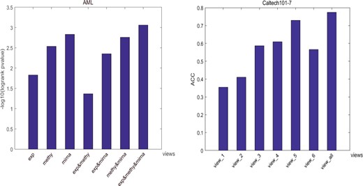
Clustering performances of CGGA using data from specific views instead of all views

Effects of the number of layers in GAEs. We also tested the influences of the number of layers stacked in GAEs on the clustering performance. Figure 3 illustrated the performance variations on the four cancer datasets as well as Caltech101-7 with respect to the number of layers. We can see that the performance on AML and Caltech101-7 is relatively stable as the number of layers increases, while on Breast, GBM and Liver datasets, the performance reduces sharply when the number of layers increases to 7 or 8. This might be due to the difficulties to train a more complex network architecture and higher risks of information loss. In summary, we only use two layers in our model as it is enough to obtain satisfactory results.

Fig. 3.

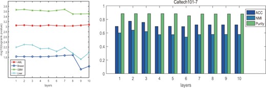
Effects of the number of layers on the clustering performance

Parameter analysis. There are two hyper-parameters λ and β in our objective function, where β can be adaptively determined by the number of neighbors k. Therefore, we investigated their impacts on the clustering performance of the proposed method on two datasets, AML and Caltech101-7 (Fig. 4). The analysis results on other datasets were provided in Supplementary Figure S1–S6. It can be observed that, the proposed method is relatively stable with respect to the two parameters on the generic machine learning datasets. For cancer datasets, the optimal values for the two parameters are dependent on the specific dataset. In general, λ can be set in the range [0.01, 10] while k can be selected from {7, 9}.

Fig. 4.

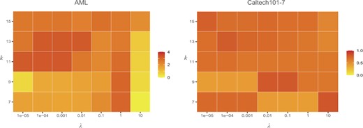
Impacts of λ and k on the clustering performance of CGGA on AML and Caltech101-7 datasets

Convergence analysis. Since our method mainly consists of two components, we first investigated the convergence of each sub-optimization problem separately. Specifically, in the first step, we can obtain the closed-form optimal solution for W according to Equation (5). In the second step, the optimization for A^v is guaranteed to converge to an optimal solution as the Hessian matrix of the Lagrange function of Equation (9) is positive definite. Similarly, we can derive the same conclusion for the optimization of S. Therefore, our algorithm can converge to an optimal solution at each iteration. Unfortunately, since the input similarity matrix A^v varies at each iteration, it is difficult to theoretically prove the overall convergence of the proposed algorithm. However, in practice, we find that our algorithm can quickly reach a stable state in practice in most cases (Fig. 5, Supplementary Figs S7–S12), which ensures the utility of our method.

Fig. 5.

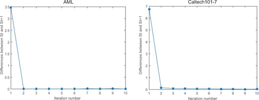
Convergence analysis of CGGA on Caltech101-7 and AML datasets. The vertical axis represents the differences between the consensus matrices S_t and S_t+1, where t is the number of overall iterations

3.4 Comparison of clusters to established subtypes

In this subsection, we investigated the connections between the clustering results identified by our method with previously established subtypes for GBM dataset. Specifically, Brennan et al. identified four major subtypes, i.e. Classical, Mesenchymal, Neural, Proneural, based on the gene expression profiles, where they further divided the Proneural subtype into proneural G-CIMP and proneural-non-G-CIMP subtypes in terms of the DNA methylation profiles(Brennan et al., 2013). We therefore reported the overall number of samples of Proneural subtype by taking the G-CIMP into account. After filtering, we retained 271 common samples with reported subtype information and the comparison results were listed in Table 6. We can observe that Subtype 1 is enriched for the Classical subtype while Subtype 2 is mainly dominated by the Proneural subtype. Subtype 3 contains samples belonging to the Mesenchymal subtype and the Neural subtype. Similar conclusions were also drawn from a smaller sample collection (Verhaak et al., 2010) (Supplementary File S1, Supplementary Table S5). Our findings indicated that patients of the Neural subtype have similar molecular traits with Mesenchymal and Classical subtypes and might be clustered together for better treatment.

Table 6.

Comparison of GBM subtypes identified by CGGA to gene expression subtypes reported by Brennan et al.

	Classical	Mesenchymal	Neural	Proneural
No of Subtype1	56	11	15	3
No of Subtype2	2	3	6	62
No of Subtype3	12	69	25	7

3.5 Clinical implications of the identified clusters

With the identified subtypes for cancer samples, we can carry out further analysis to discover the underlying differences between cancer subtypes and thus facilitate clinical therapeutics. To this end, we examined the responses of patients from different GBM subtypes to the same treatment. Specifically, the drug treatment information for GBM patients were downloaded from TCGA. After filtering, there were in total 272 samples with matched treatment data. Among these, 87 were treated with Temozolomide, an anti-cancer chemotherapy drug that is frequently used to treat brain tumors (Table 7). We then tested for each identified subgroupthe survival time of patients treated versus those not treated with the drug by using R package survminer and reported the P-vlaue of the logrank test (Fig. 6). Notably, among the three subtype groups, only patients from subtype 1 had positive responses to the drug treatment with significantly increased survival time, while for the other groups there were no significant differences detected in survival time. These results indicated that different subtypes may respond differently to certain pharmacotherapies.

Fig. 6.

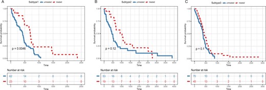
Kaplan-Meier survival analysis within each identified subtype group for GBM. Red line and blue line represent treated and untreated patients with the drug Temozolomide, respectively

Table 7.

The number of samples with drug treatment in each subtype

No. of samples	Subtype 1	Subtype 2	Subtype 3	Total
Treated	23	19	45	87
Untreated	62	53	70	185

To gain further insights into the characteristics of each subtype, we identified a set of differentially expressed genes (adjusted P-value < 0.01) associated with each subgroup using R package limma(Ritchie et al., 2015). The identified genes were then divided into down-regulated and up-regulated genes according to their fold changes and were used for the subsequent functional enrichment analysis using R package clusterProfiler(Yu et al., 2012). Figure 7 demonstrated the over-representation analysis for both GO terms and KEGG pathways. Interestingly, we found that although the enriched GO categories as well as the KEGG pathways with respect to subtype 2 and subtype 3 were similar, their associated genes exhibited opposite expression profiles. This might explain why samples of subtype 2 and subtype 3 had different responses with the same treatment.

Fig. 7.

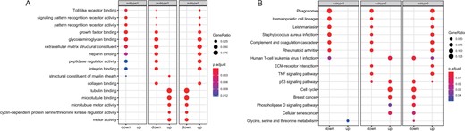
Enrichment analysis of the differentially expressed genes identified between subtypes: (A) GO functional enrichment analysis. (B) KEGG pathways over-representation analysis. Genes are divided into down-/up-regulated groups according to their fold change between different subtypes

4 Conclusions

To accurately identify cancer subtypes and facilitate precision cancer diagnosis, it is imperative to take an integrative approach that combines multi-omics data to uncover the consensus information hidden in these data. In this article, we proposed a consensus guided graph autoencoder to cluster cancer patients into biologically meaningful groups. Our method effectively learns a latent representation for each omic by graph autoencoders and then obtained a consensus similarity matrix based on the new features. Moreover, an omic-specific similarity matrix was also learned together with the consensus matrix and was further used to conduct the training process of graph autoencoders. As a result, the latent representation learning and consensus matrix learning could be enhanced with each other in an iterative manner. Extensive experimental results on both machine learning datasets and cancer datasets confirmed the superiority of our method over existing baselines. We also analyzed the clinical implications of the obtained subgroups for GBM. Specifically, the GO and KEGG enrichment analysis on the differentially expressed genes associated with each subtype exhibited distinct expression profiles, which further confirmed the importance of cancer subtype identification in cancer treatment. Taken together, we provided a new avenue to identify cancer subtypes via consensus guided graph autoencoders.

The superior performance of our method can be attributed to the following two reasons. First, we utilized GAEs to obtain robust latent representations for each omic, where both the feature information and graph structure information of samples were incorporated into a unified learning framework. Second, we proposed an effective two-step strategy to share the consistency among multiple omics and enhance the representation learning by iteratively updating the input similarity matrices for GAEs. Although effective, there also exist some limitations in our model that need further investigation. For example, two parameters are involved in our objective function and should be carefully tuned during the experiments to reach optimal solutions. Besides, the incorporation of multi-omics datasets does not necessarily lead to better clustering results in certain occasions and thus it remains challenging to uncover both the consistent and complementary information hidden in each type of multi-omics data.

Acknowledgements

The authors thank anonymous reviewers for their valuable suggestions.

Funding

This work was supported by the National Natural Science Foundation of China [61873089, 61772313, U1836216] and the Major Fundamental Research Project of Shandong Province [ZR2019ZD03].

Conflict of Interest: none declared.