Bipartite tight spectral clustering (BiTSC) algorithm for identifying conserved gene co-clusters in two species

Abstract

Motivation

Gene clustering is a widely used technique that has enabled computational prediction of unknown gene functions within a species. However, it remains a challenge to refine gene function prediction by leveraging evolutionarily conserved genes in another species. This challenge calls for a new computational algorithm to identify gene co-clusters in two species, so that genes in each co-cluster exhibit similar expression levels in each species and strong conservation between the species.

Results

Here, we develop the bipartite tight spectral clustering (BiTSC) algorithm, which identifies gene co-clusters in two species based on gene orthology information and gene expression data. BiTSC novelly implements a formulation that encodes gene orthology as a bipartite network and gene expression data as node covariates. This formulation allows BiTSC to adopt and combine the advantages of multiple unsupervised learning techniques: kernel enhancement, bipartite spectral clustering, consensus clustering, tight clustering and hierarchical clustering. As a result, BiTSC is a flexible and robust algorithm capable of identifying informative gene co-clusters without forcing all genes into co-clusters. Another advantage of BiTSC is that it does not rely on any distributional assumptions. Beyond cross-species gene co-clustering, BiTSC also has wide applications as a general algorithm for identifying tight node co-clusters in any bipartite network with node covariates. We demonstrate the accuracy and robustness of BiTSC through comprehensive simulation studies. In a real data example, we use BiTSC to identify conserved gene co-clusters of Drosophila melanogaster and Caenorhabditis elegans, and we perform a series of downstream analysis to both validate BiTSC and verify the biological significance of the identified co-clusters.

Availability and implementation

The Python package BiTSC is open-access and available at https://github.com/edensunyidan/BiTSC.

Supplementary information

Supplementary data are available at Bioinformatics online.

1 Introduction

In computational biology, a long-standing problem is how to predict functions of the majority of genes that have not been well understood. This prediction task requires borrowing functional information from other genes with similar expression patterns in the same species or orthologous genes in other species. Within a species, how to identify genes with similar expression patterns across multiple conditions is a clustering problem, and researchers have successfully used clustering methods to infer unknown gene functions (Lee, 2004; Ruan et al., 2010). Specifically, functions of less well-understood genes are inferred from known functions of other genes in the same cluster. The rationale is that genes in one cluster are likely to encode proteins in the same complex or participate in a common metabolic pathway and thus share similar biological functions (Stuart et al., 2003). In the past two decades, gene clustering for functional prediction has been empowered by the availability of abundant microarray and RNA-seq data (Bergmann et al., 2003; Le et al., 2010; Mortazavi et al., 2008; Söllner et al., 2017; Wang et al., 2009). Cross-species analysis is another approach to infer gene functions by borrowing functional information of orthologous genes in other species, under the assumption that orthologous genes are likely to share similar functions (Chen et al., 2016; Dede and Oğul, 2013; Fujibuchi et al., 2000; Kristiansson et al., 2013; Le et al., 2010; Sudmant et al., 2015). Although computational prediction of orthologous genes remains an ongoing challenge, gene orthology information with increasing accuracy is readily available in public databases such as TreeFam (Schreiber et al., 2014) and PANTHER (Mi et al., 2019). Hence, it is reasonable to combine gene expression data with gene orthology information to increase the accuracy of predicting unknown gene functions.

Given two species, the computational task is to identify conserved gene co-clusters containing genes from both species. The goal is to make each co-cluster enriched with orthologous gene pairs and ensure that its genes exhibit similar expression patterns in each species. Among existing methods for this task, the earlier methods (Snel et al., 2004; Teichmann and Babu, 2002; van Noort et al., 2003) took a two-step approach: in step 1, genes are clustered in each species based on gene expression data; in step 2, the gene clusters from the two species are paired into co-clusters based on gene orthology information. This two-step approach has a major drawback: there is no guarantee that gene clusters found in step 1 can be paired into meaningful co-clusters in step 2. The reason is that step 1 performs separate gene clustering in the two species without accounting for gene orthology, and as a result, any two gene clusters from different species may share few orthologs and should not be paired into a co-cluster. More recent methods abandoned this two-step approach. For example, SCSC (Cai et al., 2010) took a model-based approach, and MVBC (Sun et al., 2016) took a joint matrix factorization approach. Both SCSC and MVBC require that genes in two species are in one-to-one ortholog pairs. This notable limitation prevents SCSC and MVBC from considering the majority of genes that do not have known orthologs or have more than one ortholog in the other species. Furthermore, SCSC assumes that each orthologous gene pair has expression levels generated from a Gaussian mixture model and the gene expression levels are independent between the two species. This strong distributional assumption does not hold for gene expression data from RNA-seq experiments. MVBC is also limited by its required input of verified gene expression patterns, which are often unavailable for many gene expression datasets. OrthoClust (Yan et al., 2014) is a network-based gene co-clustering method that constructs a unipartite gene network with nodes as genes in two species. Edges are established based on gene co-expression relationships to connect genes of the same species, or gene orthology relationships to connect genes from different species. OrthoClust identifies gene clusters from this network using a modularity maximization approach, which cannot guarantee that each identified cluster contains genes from both species. There are also two open questions regarding the use of OrthoClust in practice: (i) how to define within-species edges based on gene co-expression and (ii) how to balance the relative weights of within-species edges and between-species edges in clustering. Another class of methods is biological network alignment (Neyshabur et al., 2013; Saraph and Milenković, 2014; Singh et al., 2008; Sun et al., 2015), whose aim is to find conserved node and edge mapping between networks of different species. These methods have been mostly applied to protein–protein interaction networks. If applied to gene co-clustering, they would have the same requirement as OrthoClust has for pre-computed within-species gene networks, whose construction from gene expression data, however, has no gold standards.

Here, we propose bipartite tight spectral clustering (BiTSC), a novel cross-species gene co-clustering algorithm, to overcome the above-mentioned disadvantages of the existing methods. BiTSC for the first time implements a bipartite-network formulation to tackle the computational task: it encodes gene orthology as a bipartite network and gene expression data as node covariates. This formulation was first mentioned by Razaee et al. (2019) but not implemented. BiTSC implements this formulation to simultaneously leverage gene orthology and gene expression data to identify tight gene co-clusters, each of which contains similar gene expression patterns in each species and rich gene ortholog pairs between species. Existing bipartite network clustering methods, which were developed for general bipartite networks, are not well suited for this task. Some of them cannot account for node covariate information (Dhillon, 2001; Larremore et al., 2014; Nie et al., 2017), while others have strong distributional assumptions that do not hold for gene orthology networks and gene expression data measured by RNA-seq (Razaee et al., 2019; Whang et al., 2013). In contrast, BiTSC adopts and combines the advantages of multiple unsupervised learning techniques, including kernel enhancement (Razaee, 2017), bipartite spectral clustering (Dhillon, 2001), consensus clustering (Monti et al., 2003), tight clustering (Tseng and Wong, 2005) and hierarchical clustering (Johnson, 1967). As a result, BiTSC has three main advantages. First, BiTSC is the first gene co-clustering method that does not force every gene into a co-cluster; in other words, it only identifies tight gene co-clusters and allows for unclustered genes. This is advantageous because some genes have individualized functions (Koonin, 2005; Ohno, 1970; Tatusov, 1997) and thus should not be assigned into any co-cluster. BiTSC is also flexible in allowing users to adjust the tightness of its identified gene co-clusters. Second, BiTSC is able to consider all the genes in two species, including those genes that do not have orthologs in the other species. Third, BiTSC takes an algorithmic approach that does not rely on any distributional assumptions, making it a robust method. Moreover, we want to emphasize that BiTSC is not only a bioinformatics method but also a general algorithm for network analysis. It can be used to identify tight node co-clusters in a bipartite network with node covariates.

2 Materials and methods

2.1 Bipartite network formulation of gene co-clustering

BiTSC formulates the cross-species gene co-clustering problem as a community detection problem in a bipartite network with node covariates. A bipartite network contains two sides of nodes, and edges only exist between nodes on different sides, not between nodes on the same side. Each node is associated with a covariate vector, also known as node attributes. In bipartite network analysis, the community detection task is to divide nodes into co-clusters based on edges and node covariates, so that nodes in one co-cluster have dense edge connections and similar node covariates on each side (Razaee et al., 2019). In its formulation, BiTSC encodes genes of two species as nodes of two sides in a bipartite network, where an edge indicates that the two genes it connects are orthologous; BiTSC encodes each gene’s expression levels as its node covariates, with the requirement that all genes in one species have expression measurements in the same set of biological samples. For the rest of the Section 2, the terms ‘nodes’ and ‘genes’ are used interchangeably, so are ‘sides’ and ‘species,’ as well as ‘node covariates’ and ‘gene expression levels.’

In mathematical notations, there are m and n nodes on sides 1 and 2, respectively. Edges are represented by a binary bi-adjacency matrix $\mathbf{A}={(a_{ij})}_{m\times n}$⁠, where a_ij = 1 indicates that there is an edge between node i on side 1 and node j on side 2, i.e. gene i from species 1 and gene j from species 2 are orthologous. Note that A is allowed to be a weighted bi-adjacency matrix with $a_{ij}\in [0,1]$ when weighted orthologous relationships are considered. Node covariates are encoded in two matrices, ${\mathbf{X}}_1$ and ${\mathbf{X}}_2$⁠, which have dimensions $m\times p_1$ and $n\times p_2$⁠, respectively, i.e. species 1 and 2 have gene expression levels measured in p₁ and p₂ biological samples, respectively. The ith row of ${\mathbf{X}}_1$ is denoted as ${\mathbf{x}}_{1i}^T$⁠, and similarly for ${\mathbf{X}}_2$⁠. Note that all vectors are column vectors unless otherwise stated.

2.2 The BiTSC algorithm

BiTSC is a general algorithm that identifies tight node clusters from a bipartite network with node covariates. Table 1 summarizes the input data, input parameters and output of BiTSC. Figure 1 illustrates the idea of BiTSC, and Supplementary Figure S4 shows the detailed workflow. In the context of cross-species gene co-clustering, BiTSC inputs $\mathbf{A}$⁠, which contains gene orthology information, and ${\mathbf{X}}_1$ and ${\mathbf{X}}_2$⁠, which denote gene expression data in species 1 and 2. BiTSC outputs tight gene co-clusters such that genes within each co-cluster are rich in orthologs and share similar gene expression levels across multiple biological samples in each species. A unique advantage of BiTSC is that it does not force all genes into co-clusters and allows certain genes with few orthologs or outlying gene expression levels to stay unclustered.

Table 1.

Input and output of BiTSC

Input data: bipartite network with node covariates   • A: m × n bi-adjacency matrix • X1: m × p1 covariate matrix for side 1 • X2: m × p2 covariate matrix for side 2   Input parameters:   • H: number of subsampling runs • $\rho \in (0,1)$⁠: proportion of nodes to subsample in each run • τ: tuning parameter for constructing the enhanced bi-adjacency matrix • K0: number of node co-clusters to identify in each run • $\alpha \in (0,1)$⁠: tightness parameter   Output:   • Tight node co-clusters that are mutually exclusive subsets of the $(m+n)$ nodes

Fig. 1.

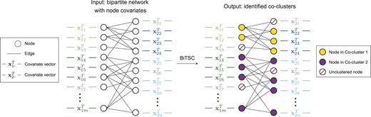
Diagram illustrating the input and output of BiTSC. The identified tight node co-clusters satisfy that, within any co-cluster, nodes on the same side share similar covariates, and nodes from different sides are densely connected. In the context of gene co-clustering, within any co-cluster, genes from the same species share similar gene expression levels across multiple conditions, and genes from different species are rich in orthologs

As an overview, BiTSC is an ensemble algorithm that takes multiple parallel runs. In each run, BiTSC first identifies initial node co-clusters in a randomly subsampled bipartite subnetwork; next, it assigns the unsampled nodes to these initial co-clusters based on node covariates. Then BiTSC aggregates the sets of node co-clusters resulted from these multiple runs into a consensus matrix, from which it identifies tight node co-clusters by hierarchical clustering. This subsampling-and-aggregation idea was inspired by consensus clustering (Monti et al., 2003) and tight clustering (Tseng and Wong, 2005).

BiTSC has five input parameters (Table 1): H, the number of subsampling runs; $\rho \in (0,1)$⁠, the proportion of nodes to subsample in each run; τ, the tuning parameter for constructing the enhanced bi-adjacency matrix; K₀, the number of node co-clusters in each run; $\alpha \in (0,1)$⁠, the tightness parameter used to find tight node co-clusters in the last step. In the hth run, $h=1,\dots ,H$⁠, BiTSC has the following four steps.

1. Subsampling. BiTSC randomly samples without replacement $\tilde{m}=\lfloor \rho m\rfloor$ nodes on side 1 and $\tilde{n}=\lfloor \rho n\rfloor$ nodes on side 2, where the floor function $\lfloor x\rfloor$ gives the largest integer less than or equal to x. We denote the subsampled bi-adjacency matrix as $\tilde{\mathbf{A}}$⁠, whose dimensions are $\tilde{m}\times \tilde{n}$⁠, and the two subsampled covariate matrices as ${\tilde{\mathbf{X}}}_1$ and ${\tilde{\mathbf{X}}}_2$⁠, whose dimensions are $\tilde{m}\times p_1$ and $\tilde{n}\times p_2$⁠, respectively.

2. Kernel enhancement. To find initial node co-clusters from this bipartite subnetwork $\tilde{\mathbf{A}}$ with node covariates ${\tilde{\mathbf{X}}}_1$ and ${\tilde{\mathbf{X}}}_2$⁠, a technical issue is that this subnetwork may have sparse edges and disconnected nodes. To address this issue, BiTSC uses the kernel enhancement technique proposed by Razaee (2017) to complement network edges by integrating node covariates. This kernel enhancement step will essentially reweight edges by incorporating pairwise node similarities on both sides. Technically, BiTSC defines two kernel matrices ${\tilde{\mathbf{K}}}_1$ and ${\tilde{\mathbf{K}}}_2$⁠, which are symmetric and have dimensions $\tilde{m}\times \tilde{m}$ and $\tilde{n}\times \tilde{n}$⁠, for nodes on sides 1 and 2, respectively. In ${\tilde{\mathbf{K}}}_r$⁠, r = 1, 2, the (i, j)th entry is $k_r({\tilde{\mathbf{x}}}_{ri},{\tilde{\mathbf{x}}}_{rj})=\text{exp}\hspace{0.17em}(-||{\tilde{\mathbf{x}}}_{ri}-{\tilde{\mathbf{x}}}_{rj}|{|}^2/p_r)$⁠, where $\left|\right|{\tilde{\mathbf{x}}}_{ri}-{\tilde{\mathbf{x}}}_{rj}\left|\right|$ is the Euclidean distance between nodes i and j on side r in this subnetwork. Then BiTSC constructs an enhanced bi-adjacency matrix $\tilde{\mathbf{B}}=({\tilde{\mathbf{K}}}_1+{\tau }_1{\mathbf{I}}_{\tilde{m}})\tilde{\mathbf{A}}({\tilde{\mathbf{K}}}_2+{\tau }_2{\mathbf{I}}_{\tilde{n}})$⁠, whose dimensions are $\tilde{m}\times \tilde{n}$⁠, where ${\mathbf{I}}_{\tilde{m}}$ and ${\mathbf{I}}_{\tilde{n}}$ are the $\tilde{m}$- and $\tilde{n}$-dimensional identity matrices, and $\tau =({\tau }_1,{\tau }_2)\in {[0,\infty )}^2$ is a tuning parameter that balances the information from the subsampled bi-adjacency matrix and the two kernel matrices. Since $\tilde{\mathbf{B}}$ can be rewritten as ${\tilde{\mathbf{K}}}_1\tilde{\mathbf{A}}{\tilde{\mathbf{K}}}_2+{\tau }_1\tilde{\mathbf{A}}{\tilde{\mathbf{K}}}_2+{\tau }_2{\tilde{\mathbf{K}}}_1\tilde{\mathbf{A}}+{\tau }_1{\tau }_2\tilde{\mathbf{A}}$⁠, when τ₁ and τ₂ are large, ${\tau }_1{\tau }_2\tilde{\mathbf{A}}$ dominates and covariate information has little to no impact on $\tilde{\mathbf{B}}$⁠; when τ₁ and τ₂ are both close to 0, ${\tilde{\mathbf{K}}}_1\tilde{\mathbf{A}}{\tilde{\mathbf{K}}}_2$ dominates and covariate information contributes more to the enhanced bi-adjacency matrix.

3. Bipartite spectral clustering. BiTSC identifies initial node co-clusters from $\tilde{\mathbf{B}}$⁠, the enhanced bi-adjacency matrix of the bipartite subnetwork, by borrowing the idea from Dhillon (2001). Technically, BiTSC first constructs

   $$\tilde{\mathbf{W}}={\left({\tilde{w}}_{ij}\right)}_{(\tilde{m}+\tilde{n})\times (\tilde{m}+\tilde{n})}=\left[\begin{array}{cc}{\mathbf{0}}_{\tilde{m}\times \tilde{m}}& {\tilde{\mathbf{B}}}_{\tilde{m}\times \tilde{n}}\\ {\tilde{\mathbf{B}}}_{\tilde{n}\times \tilde{m}}^T& {\mathbf{0}}_{\tilde{n}\times \tilde{n}}\end{array}\right]\hspace{0.17em},$$

   (1)

which may be viewed as the adjacency matrix of a unipartite network with $(\tilde{m}+\tilde{n})$ nodes. Then BiTSC identifies K₀ mutually exclusive and collectively exhaustive clusters from $\tilde{\mathbf{W}}$ via normalized spectral clustering (Ng et al., 2001) as follows:

• BiTSC computes a degree matrix $\tilde{\mathbf{D}}$⁠, an $(\tilde{m}+\tilde{n})$-dimensional diagonal matrix whose diagonal entries are the row sums of $\tilde{\mathbf{W}}$⁠.

• BiTSC computes the normalized Laplacian of $\tilde{\mathbf{W}}$ as $\tilde{\mathbf{L}}={\mathbf{I}}_{\tilde{m}+\tilde{n}}-{\tilde{\mathbf{D}}}^{-\frac{1}{2}}\tilde{\mathbf{W}}{\tilde{\mathbf{D}}}^{-\frac{1}{2}}$⁠. Note that $\tilde{\mathbf{L}}$ is a positive semi-definite $(\tilde{m}+\tilde{n})\times (\tilde{m}+\tilde{n})$ matrix with $(\tilde{m}+\tilde{n})$ non-negative real-valued eigenvalues: $0={\lambda }_1\le \cdots \le {\lambda }_{\tilde{m}+\tilde{n}}$⁠.

• BiTSC finds the first K₀ eigenvectors of $\tilde{\mathbf{L}}$ that correspond to ${\lambda }_1,\dots ,{\lambda }_{K_0}$⁠. Each eigenvector has length $(\tilde{m}+\tilde{n})$⁠. Then BiTSC collects these K₀ eigenvectors column-wise into a matrix $\tilde{\mathbf{U}}$⁠, whose dimensions are $(\tilde{m}+\tilde{n})\times K_0$⁠.

• BiTSC normalizes each row of $\tilde{\mathbf{U}}$ to have a unit ${\ell }_2$ norm and denotes the normalized matrix as $\tilde{\mathbf{V}}$⁠. Specifically, $\tilde{\mathbf{V}}$ also has dimensions $(\tilde{m}+\tilde{n})\times K_0$⁠, and its ith row ${\tilde{\mathbf{v}}}_i^T={\tilde{\mathbf{u}}}_i^T/\left|\right|\tilde{\mathbf{u}}i\left|\right|$⁠, where ${\tilde{\mathbf{u}}}_i^T$ is the ith row of $\tilde{\mathbf{U}}$ and $\left|\right|·\left|\right|$ denotes the ${\ell }_2$ norm.

• BiTSC applies K-means clustering to divide the $(\tilde{m}+\tilde{n})$ rows of $\tilde{\mathbf{V}}$ into K₀ clusters. In detail, Euclidean distance is used to measure the distance between each row and each cluster center.

The resulting K₀ clusters of $(\tilde{m}+\tilde{n})$ nodes are regarded as the initial K₀ node co-clusters.

• 4. Assignment of unsampled nodes. BiTSC assigns the unsampled nodes, which are not subsampled in step 1, into the initial K₀ node co-clusters. Specifically, there are $(m-\tilde{m})$ and $(n-\tilde{n})$ unsampled nodes on sides 1 and 2, respectively. For each initial node co-cluster, BiTSC first calculates a mean covariate vector on each side. For example, if a co-cluster contains nodes i and j on side 1 of the bipartite subnetwork, its mean covariate vector on side 1 would be computed as $({\tilde{\mathbf{x}}}_{1i}+{\tilde{\mathbf{x}}}_{1j})/2$⁠. BiTSC next assigns each unsampled node to the co-cluster whose mean covariate vector (on the same side as the unsampled node) has the smallest Euclidean distance to the node’s covariate vector.

With the above four steps, in the hth run, $h=1,\dots ,H$⁠, BiTSC obtains K₀ node co-clusters, which are mutually exclusive and collectively containing all the m nodes on side 1 and n nodes on side 2. To aggregate the H sets of K₀ node co-clusters, BiTSC first constructs a node co-membership matrix for each run. Specifically, ${\mathbf{M}}^{(h)}={(m_{ij}^{(h)})}_{(m+n)\times (m+n)}$ denotes a node co-membership matrix resulted from the hth run. ${\mathbf{M}}^{(h)}$ is a binary and symmetric matrix indicating the pairwise cluster co-membership of the $(m+n)$ nodes. That is, an entry in ${\mathbf{M}}^{(h)}$ is 1 if the two nodes corresponding to its row and column are assigned to the same co-cluster; otherwise, it is 0. Then BiTSC constructs a consensus matrix $\overline{\mathbf{M}}={({\overline{m}}_{ij})}_{(m+n)\times (m+n)}$ by averaging ${\mathbf{M}}^{(1)},\dots ,{\mathbf{M}}^{(H)}$⁠, i.e. ${\overline{m}}_{ij}=\sum _{h=1}^H{m}_{ij}^{(h)}/H\in [0,1]$⁠. An entry of $\overline{\mathbf{M}}$ indicates the frequency that the two nodes corresponding to its row and column are assigned to the same co-cluster, among the H runs.

Finally, BiTSC identifies tight node co-clusters from $\overline{\mathbf{M}}$ such that within every co-cluster, all pairs of nodes have been previously clustered together at a frequency of at least α, the input tightness parameter. Specifically, BiTSC considers $(1-\overline{\mathbf{M}})$ as a pairwise distance matrix of $(m+n)$ nodes. Then BiTSC applies hierarchical clustering with complete linkage to $(1-\overline{\mathbf{M}})$⁠, and it subsequently cuts the resulting dendrogram at the distance threshold $(1-\alpha )$⁠. This guarantees that all the nodes within each resulting co-cluster have pairwise distances no greater than $(1-\alpha )$⁠, which is equivalent to being previously clustered together at a frequency of at least α. A larger α value will lead to finer co-clusters, i.e. a greater number of smaller clusters and unclustered nodes. BiTSC provides a visualization-based approach to help users choose α: for each candidate α value, BiTSC collects the nodes in the resulting tight co-clusters and plots a heatmap of the submatrix of $\overline{\mathbf{M}}$ that corresponds to these nodes; users are encouraged to pick an α value whose resulting number of tight co-clusters is close to the number of visible diagonal blocks in the heatmap. (Please see Supplementary Materials for a demonstration in the real data example in Section 3.2) Regarding the choice of K₀, i.e. the input number of co-clusters in each run, the entries of $\overline{\mathbf{M}}$ provide a good guidance. A reasonable K₀ should lead to many entries equal to 0 or 1 and few having fractional values in between (Monti et al., 2003). Following this reasoning, BiTSC implements a computationally efficient algorithm to automatically choose K₀ (Algorithm S1 in Supplementary Section S6) while also giving users the option to input their preferred K₀ value. In Supplementary Section S6, we demonstrate the use of Algorithm S1 for the real data application (Section 3.2).

To summarize, BiTSC leverages joint information from bipartite network edges and node covariates to identify tight node co-clusters that are robust to data perturbation, i.e. subsampling. In its application to gene co-clustering, BiTSC integrates gene orthology information with gene expression data to identify tight gene co-clusters, which are enriched with orthologs and contain genes of similar expression patterns in both species. In particular, within each subsampling run, the bipartite spectral clustering step identifies co-clusters enriched with orthologs; another two steps, the kernel enhancement and the assignment of unsampled nodes, ensure that genes with similar expression patterns in each species tend to be clustered together. Moreover, the subsampling-and-aggregation approach makes the output tight gene co-clusters robust to the existence of outlier genes, which may have few orthologs or exhibit outlying gene expression patterns. The pseudocode of BiTSC is in Algorithm 1.

Algorithm 1 Pseudocode of BiTSC

• For h = 1 to H:

  1. Subsample $\tilde{m}=\lfloor \rho m\rfloor$ nodes from side 1 and $\tilde{n}=\lfloor \rho n\rfloor$ nodes from side 2 to obtain a subsampled bi-adjacency matrix $\tilde{\mathbf{A}}$ and two subsampled node covariate matrices ${\tilde{\mathbf{X}}}_1$ and ${\tilde{\mathbf{X}}}_2$

  2. Use kernel enhancement to construct an enhanced bi-adjacency matrix $\tilde{\mathbf{B}}$ from $\tilde{\mathbf{A}},\hspace{0.17em}{\tilde{\mathbf{X}}}_1$ and ${\tilde{\mathbf{X}}}_2$

  3. Find K₀ initial node co-clusters from $\tilde{\mathbf{B}}$ by bipartite spectral clustering

  4. Obtain K₀ node co-clusters by assigning the unsampled nodes into the K₀ initial node co-clusters; encode the K₀ node co-clusters as a co-membership matrix ${\mathbf{M}}^{(h)}$

• Calculate the consensus matrix $\overline{\mathbf{M}}$ as the average of ${\mathbf{M}}^{(1)},\dots ,{\mathbf{M}}^{(H)}$

• Identify tight node co-clusters from $\overline{\mathbf{M}}$ with tightness parameter α

3 Results

3.1 Simulation validates the design, performance and robustness of BiTSC

We designed multiple simulation studies to justify the algorithm design of BiTSC by comparing it with the six possible variants listed in Supplementary Section S1: spectral-kernel, spectral, BiTSC-1, BiTSC-1-nokernel, BiTSC-1-NC and BiTSC-1-NC-nokernel.

We use the weighted Rand index (Thalamuthu et al., 2006), defined in Supplementary Section S3, as the evaluation measure of co-clustering results. The weighted Rand index compares two sets of node co-clusters: the co-clusters found by an algorithm and the true co-clusters used to generate data, and outputs a value between 0 and 1, with a value of 1 indicating perfect agreement between the two sets. The weighted Rand index is a proper measure for evaluating BiTSC and its variants because it accounts for noise nodes that do not belong to any co-clusters.

We compared BiTSC with its six possible variants in identifying node co-clusters from simulated networks with varying levels of noise nodes (i.e. θ in Supplementary Section S2) and varying average degrees of nodes. It is expected that the identification would become more difficult as the level of noise nodes increases or as the average degree decreases. Our results in Figure 2a are consistent with this expectation. Figure 2a also shows that BiTSC consistently outperforms its six variant algorithms at all noise node levels and average degrees greater than five. This phenomenon is reasonable because BiTSC performs subsampling on the network, and the subsampled network, if too sparse, would make the bipartite spectral clustering algorithm fail. In fact, the three algorithms that outperform BiTSC for sparse networks, i.e. spectral-kernel, BiTSC-1 and BiTSC-1-NC, only perform bipartite spectral clustering on the entire network, so they are more robust to network sparsity. In addition, we observe that the three variants that do not use kernel enhancement consistently have the worst performance. In summary, BiTSC has a clear advantage over its possible variants in the existence of noise nodes and when the network is not overly sparse. These results confirm the effectiveness of the subsampling-and-aggregation approach and the kernel enhancement step, and they also show that subsampling in the first step is beneficial if the network is not too sparse, thus justifying the design of BiTSC.

Fig. 2.

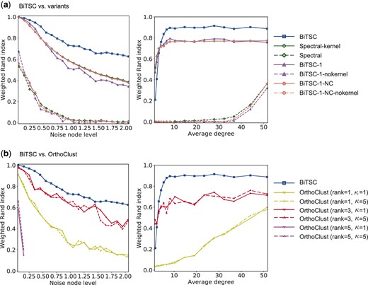
Performance of BiTSC versus (a) its six variant algorithms (Supplementary Section S1) and (b) OrthoClust. The weighted Rand index is plotted as a function of noise node level (first column) or average degree (second column). The datasets are simulated using the approach described in Supplementary Section S2. For both columns, we set K = 15, $n_1=50,\hspace{0.17em}{n}_2=70,\hspace{0.17em}{p}_1=p_2=2,\hspace{0.17em}{\sigma }_1={\sigma }_2=10$ and ${\omega }_1={\omega }_2=0.1$⁠. For the first column, we vary the noise node level θ from 0.05 to 2.05 and set p = 0.15 and q = 0.03. For the second column, we set $\theta =0.5$⁠, vary p from 0.005 to 0.175, set $q=p/5$⁠, and as a result vary the average degree from 1 to 51 (see Supplementary Section S2.1 for details about the average degree). For the input parameters of BiTSC and its variants, we choose $H=50,\rho =0.8,\tau =(1,1),K_0=K=15$ and $\alpha =0.7$ whenever applicable. We set $K_0=K$ following the convention that when the ground truth is known in simulation studies, one can select input parameters based on the truth (Karrer and Newman, 2011; Larremore et al., 2014; Razaee et al., 2019; Zhao et al., 2012). For OrthoClust, rank $=3$ means that in the construction of within-species gene co-expression networks, we connect each gene with its three closest genes in terms of Euclidean distance; similarly for rank $=1$ and rank $=5$⁠. In this figure, genes in identified co-clusters that only contain genes from one species are treated as noise genes, just like unclustered genes, in the calculation of the weighted Rand index. This is why in the second column of (b), we cannot see the curves for OrthoClust (rank $=5$⁠)—no co-clusters with genes from both species were identified. We show that BiTSC also outperforms OrthoClust when we only consider unclustered genes as noise genes in Supplementary Figure S1

In addition to validating the design of BiTSC, we also performed simulation studies to compare BiTSC with OrthoClust (Yan et al., 2014), a gene clustering method that also simultaneously uses gene expression and orthology information. We chose OrthoClust as the baseline method to compare BiTSC against because OrthoClust is the only recent method that does not (i) exclude genes not in one-to-one orthologs like SCSC (Cai et al., 2010) and MVBC (Sun et al., 2016) do or (ii) have strong distributional assumptions as SCSC does. Moreover, OrthoClust has a unipartite network formulation, so its comparison with BiTSC would inform the effectiveness of our bipartite network formulation. The OrthoClust software takes three input files: two within-species gene co-expression networks constructed by users and one between-species ortholog network. Following the recommendation in OrthoClust, we constructed the within-species gene co-expression networks by connecting each gene to its closest gene(s), whose number is specified by a tuning parameter rank, in terms of Euclidean distance. OrthoClust allows users to specify a κ value (in the between-species ortholog network input file), which balances the weights of within-species edges and between-species edges in the cost function. Our results in Figure 2b show that BiTSC consistently outperforms OrthoClust under various simulation settings.

Furthermore, we performed simulation studies to show the robustness of BiTSC to its input parameters: K₀ (the number of co-clusters to identify in each subsampling run), ρ (the proportion of nodes to subsample in each run) and $\tau =({\tau }_1,{\tau }_2)$ (the tuning parameters in the kernel enhancement step) (Supplementary Section S4). We find that BiTSC performs well when K₀ is set to be equal to or larger than K, the number of true co-clusters (Supplementary Fig. S6a). For ρ, we recommend a default value of 0.8 (Supplementary Fig. S6b). For τ, we recommend a default value of (1, 1) based on Supplementary Figures S6c and S7, which show that small τ values lead to better clustering results when the network is sparse, and that BiTSC becomes more robust to τ values when the network becomes denser. In general, small τ values put large weights on node covariates, whereas large τ values make BiTSC use more of the edge information to find node clusters. Users have the flexibility to set τ values based on their confidence or preference on node covariates and edges. For instance, if a user would like to find co-clusters such that between-species edges are dense but within-species gene expression might be dissimilar, he or she may opt for larger τ values provided that the kernel enhancement compensates the edge sparsity enough so that BiTSC can successfully run. Overall, BiTSC is robust to the specification of these tuning parameters.

3.2 BiTSC identifies gene co-clusters from Drosophila melanogaster and Caenorhabditis elegans timecourse gene expression data and predicts unknown gene functions

In this section, we demonstrate how BiTSC is capable of identifying conserved gene co-clusters of D.melanogaster (fly) and C.elegans (worm). We compared BiTSC with OrthoClust (Yan et al., 2014) and performed a series of downstream bioinformatics analysis to both validate BiTSC and verify the biological significance of its identified co-clusters. We compared BiTSC with OrthoClust and not SCSC or MVBC for the same reasons as described in Section 3.1.

3.2.1 BiTSC outperforms OrthoClust in identifying gene co-clusters with enriched ortholog pairs and similar expression levels

We applied BiTSC and OrthoClust to the D.melanogaster and C.elegans developmental-stage RNA-seq data generated by the modENCODE consortium (Gerstein et al., 2014; ,Li et al., 2014) and the gene orthology annotation from the TreeFam database (Li et al., 2006). For data processing, please see Supplementary Section S5. We ran BiTSC with input parameters H = 100, $\rho =0.8$⁠, $\tau =(1,1)$⁠, $K_0=30$ and $\alpha =0.9$⁠. For the choices of K₀ and α, please see Supplementary Section S6 and Supplementary Materials. We ran OrthoClust by following the instruction on its GitHub page (https://github.com/gersteinlab/OrthoClust accessed on November 12, 2019). Specifically, we constructed the within-species gene co-expression networks by connecting each gene with its closest five genes in terms of Pearson correlation and used κ = 1 (the default value). For details regarding the computational time of BiTSC and OrthoClust, please see Supplementary Section S8. To compare BiTSC and OrthoClust, we picked a similar number of large gene co-clusters identified by either method: 16 BiTSC co-clusters with at least 10 genes in each species (Table 2) versus 14 OrthoClust co-clusters with at least 2 genes in each species (Supplementary Table S1). Compared with OrthoClust, the co-clusters identified by BiTSC are more balanced in sizes between fly and worm. In contrast, OrthoClust co-clusters typically have many genes in one species but few genes in the other species; in particular, if we restricted the OrthoClust co-clusters to have at least 10 genes in each species, only two co-clusters would be left. We also ran OrthoClust again with κ = 3 (the value used in OrthoClust paper) instead of κ = 1, and the result is very similar (Supplementary Table S2). We evaluated both methods’ identified co-clusters in two aspects (using κ = 1 for OrthoClust): the enrichment of orthologous genes and the similarity of gene expression levels in each co-cluster. Figure 3 shows that the BiTSC co-clusters exhibit both stronger enrichment of orthologs and higher similarity of gene expression than the OrthoClust co-clusters do. Note that in general, the co-clusters identified by OrthoClust (Supplementary Table S1), with cluster sizes ranging between 184 and 1002, are larger than those identified by BiTSC (Table 2). Although the difference in cluster size does not invalidate our analysis, for further investigation, we adjusted the input parameters of BiTSC to obtain co-clusters that are closer to those identified by OrthoClust in size. With the new input parameter choices for BiTSC, we are able to further confirm the advantages of BiTSC in Supplementary Figure S11. Therefore, the gene co-clusters identified by BiTSC have better biological interpretations than their OrthoClust counterparts because of their more balanced gene numbers in two species, greater enrichment of orthologs and better grouping of genes with similar expressions.

Fig. 3.

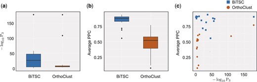
Comparison of BiTSC and OrthoClust in terms of their identified fly-worm gene co-clusters (Section 3.2.1). (a) Distributions of within-cluster enrichment of ortholog pairs. For BiTSC and OrthoClust, a boxplot is shown for the $-{\text{log}}_{10}{\mathrm{P}}_3$ values calculated by the ortholog pair enrichment test (Supplementary Section S7.3) on the identified gene co-clusters. Larger $-{\text{log}}_{10}{\mathrm{P}}_3$ values indicate stronger enrichment. (b) Distributions of within-cluster gene expression similarity. For BiTSC and OrthoClust, a boxplot is shown for the average pairwise Pearson correlation (PPC) between genes of the same species within each identified co-cluster. (c) Within-cluster gene expression similarity versus ortholog enrichment. Each point corresponds to one co-cluster identified by BiTSC or OrthoClust. The $-{\text{log}}_{10}{\mathrm{P}}_3$ and average PPC values are the same as those shown in (a) and (b)

Table 2.

Fly-worm gene co-clusters identified by BiTSC (Section 3.2)

Co-cluster	No. of fly genesa (without GOb)	No. of worm genes (without GO)	Examples BP GO terms highly enriched in both speciesc	${\mathrm{P}}_2$d	${\mathrm{P}}_3$e
1	106 (19)	83 (15)	Chemical synaptic transmission; synaptic signaling	1.35e-07	2.77e-53
2	46 (8)	119 (28)	Muscle cell development	1.70e-09	1.50e-17
3	75 (3)	83 (6)	Peptide and amide biosynthetic process	1.17e-08	6.23e-180
4	73 (4)	50 (13)	ATP metabolic process	2.72e-12	1.61e-58
5	57 (4)	62 (8)	Protein catabolic process; proteolysis	3.15e-09	3.15e-56
6	83 (4)	36 (8)	Mitochondrial translation; mitochondrial gene expression	2.60e-03	2.04e-32
7	89 (13)	25 (8)	Protein localization to endoplasmic reticulum	2.69e-10	7.72e-22
8	80 (16)	26 (11)	Ribosome biogenesis; RNA metabolic processing	2.05e-16	7.50e-37
9	29 (3)	76 (19)	Cilium and cell projection organization	2.03e-09	3.81e-05
10	32 (2)	24 (6)	DNA replication and metabolic process	2.98e-06	6.53e-02
11	25 (4)	19 (4)	DNA replication	2.46e-06	1.00e-00
12	28 (4)	15 (4)	G protein-coupled glutamate receptor signaling pathway	4.17e-14	1.81e-10
13	16 (7)	25 (12)	Glycoside catabolic process; transmembrane transport	1.52e-02	5.29e-46
14	15 (1)	24 (4)	DNA metabolic process; cell cycle process	1.83e-05	3.11e-02
15	24 (2)	11 (1)	Oxidation reduction process	1.41e-03	2.36e-31
16	14 (0)	15 (1)	Cilium organization; cell projection assembly	1.20e-07	1.83e-02

a

Number of fly genes in the co-cluster.

b

Number of fly genes without BP GO term annotations in the co-cluster.

c

Examples of BP GO terms that are highly enriched in both species in the co-cluster (Supplementary Section S7.1). These example BP GO terms are used as labels of the co-clusters in Figure 4.

d

P-value of the co-cluster based on the GO term overlap test (Supplementary Section S7.2).

e

P-value of the co-cluster based on the ortholog enrichment test (Supplementary Section S7.3).

3.2.2 Functional analysis verifies the biological significance of BiTSC gene co-clusters

We next analyzed the 16 gene co-clusters identified by BiTSC. First, we verified that genes in each co-cluster exhibit similar functions within fly and worm. We performed the GO term enrichment test (Supplementary Section S7.1) for each co-cluster in each species. The results are summarized in Supplementary Figure S2 and Supplementary Materials, which show that every co-cluster has strongly enriched GO terms with extremely small P-values, i.e. P₁ values. Hence, genes in every co-cluster indeed share similar biological functions within fly and worm. We also calculated the pairwise Pearson correlation coefficients between genes of the same species within each co-cluster (Supplementary Fig. S3). The overall high correlation values also confirm the within-cluster functional similarity in each species. Second, we show that within each co-cluster, genes share similar biological functions between fly and worm. We performed the GO term overlap test (Supplementary Section S7.2), which output small P-values, i.e. ${\mathrm{P}}_2$ values, suggesting that fly and worm genes in each co-cluster have a significant overlap in their GO terms. Supplementary Figure S2 also illustrates this functional similarity between fly and worm genes in the same co-cluster. In summary, the 16 gene co-clusters exhibit clear biological functions, some of which are conserved between fly and worm.

The above analysis results are summarized in Table 2. Specifically, for each co-cluster, Table 2 lists the numbers of fly and worm genes, the numbers of genes lacking BP GO term annotations, for example, GO terms enriched in both species by the GO term enrichment test, and P-values from the GO term overlap test and the ortholog enrichment test (Supplementary Section S7). Interestingly, we observe that when BiTSC identifies co-clusters, it simultaneously leverages gene expression similarity and gene orthology to complement each other. For example, co-clusters 10 and 11 do not have strong enrichment of orthologs but exhibit extremely high similarity of gene expression in both fly and worm; on the other hand, co-cluster 13 has relatively weak gene expression similarity but particularly strong enrichment of orthologs. This advantage of BiTSC would enable it to identify conserved gene co-clusters even based on incomplete orthology information.

We further visualized the 16 gene co-clusters using the concensus matrix $\overline{\mathbf{M}}$⁠. Figure 4 plots the fly and worm genes in these co-clusters, as well as 1000 randomly sampled unclustered genes as a background. Supplementary Figure S9 shows that the pattern of the 16 co-clusters is robust to the random sampling of unclustered genes. We observe that many co-clusters are well separated, suggesting that genes in these different co-clusters are rarely clustered together. We also see that some co-clusters are close to each other, including co-clusters 1 and 12, co-clusters 9 and 16 and co-clusters 10, 11 and 14. To investigate the reason behind this phenomenon, we inspected Table 2 and Supplementary Figure S2 to find that overlapping co-clusters share similar biological functions. This result again confirms that the identified gene co-clusters are biologically meaningful.

Fig. 4.

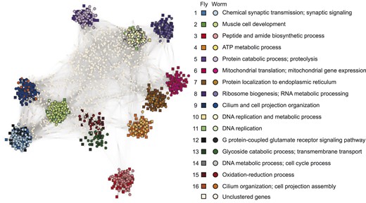
Visualization of the 16 gene co-clusters found by BiTSC from the fly-worm gene network (Section 3.2). The visualization is based on the consensus matrix $\overline{\mathbf{M}}$ using the R package igraph (Csardi and Nepusz, 2006) (https://igraph.org, the Fruchterman–Reingold layout algorithm). Genes in the 16 co-clusters are marked by distinct colors, with squares and circles representing fly and worm genes, respectively. For each co-cluster, representative BP GO terms are labeled (Table 2). 1000 randomly chosen unclustered genes are also displayed and marked in white. In this visualization, both the gene positions and the edges represent values in $\overline{\mathbf{M}}$⁠. The higher the consensus value between two genes, the closer they are positioned and the darker the edge is between them. If the consensus value is zero, then there is no edge

Moreover, we computationally validated BiTSC’s capacity to predict unknown gene functions. Many co-clusters contain genes that do not have BP GO terms. For each of these genes, we predicted its BP GO terms as its co-cluster’s top enriched BP GO terms. Then we compared the predicted BP GO terms with the gene’s other functional annotation, in particular, molecular function (MF) or cellular component (CC) GO terms. Our comparison results in Supplementary Figure S10 show that the predicted BP GO terms are highly compatible with the known MF or CC GO terms, suggesting the validity of our functional prediction based on the BiTSC co-clusters.

4 Discussion

BiTSC is a general bipartite network clustering algorithm. It is unique in identifying tight node co-clusters such that nodes in a co-cluster share similar covariates and are densely connected. In addition to cross-species gene co-clustering, BiTSC has a wide application potential in biomedical research. In general, BiTSC is applicable to computational tasks that can be formulated as a bipartite network clustering problem, where edges and node covariates jointly indicate a co-clustering structure. Here, we list three examples. The first example is the study of transcription factor (TF) co-regulation. In a TF-gene bipartite network, TFs and genes constitute nodes of two sides, an edge indicates that a TF regulates a gene, and node covariates are expression levels of TFs and genes. BiTSC can identify TF-gene co-clusters so that every co-cluster indicates a group of TFs co-regulating a set of genes. The second example is cross-species cell clustering. One may construct a biparite cell network, in which cells of one species form nodes of one side, by drawing an edge between cells of different species if the two cells are similar in some way, e.g. co-expression of orthologous genes. Node covariates may be gene expression levels and other cell characteristics. Then BiTSC can identify cell co-clusters as conserved cell types in two species. The third example is drug repurposing. One may construct a drug-target bipartite network by connecting drugs to their known targets (usually proteins) and including biochemical properties of drugs and targets as node covariates (Mei et al., 2013). BiTSC can then identify drug–target co-clusters to reveal new potential targets of drugs.

A natural generalization of BiTSC is to identify node co-clusters in a multipartite network, which has more than two types of nodes. An important application of multipartite network clustering is the identification of conserved gene co-clusters across multiple species. Here, we describe a possible way of generalizing BiTSC in this application context. Suppose that we want to identify conserved gene co-clusters across three species: Homo sapiens (human), Mus musculus (mouse) and Pan troglodytes (chimpanzee). We can encode the three-way gene orthology information in a tripartite network and include gene expression levels as node covariates. To generalize BiTSC, we may represent the tripartite network as three bi-adjacency matrices (one for human and mouse, one for human and chimpanzee, and one for mouse and chimpanzee) and three covariate matrices, one per species. A key step in this generalization is to stack three (subsampled and kernel-enhanced) bi-adjacency matrices into a unipartite adjacency matrix and apply spectral clustering. Other parts of BiTSC, such as the subsampling-and-aggregation approach, the assignment of unsampled nodes and the hierarchical clustering in the last step to identify tight co-clusters, will stay the same. We have implemented this functionality in the BiTSC software package. Compared to the existing method OrthoClust (Yan et al., 2014) that can also perform multispecies gene co-clustering, BiTSC is more transparent in its combination of gene orthology and expression information (because guidance is provided for the selection of each tuning parameter in BiTSC) and is more focused on identifying gene co-clusters rather than within-species gene clusters.

BiTSC is also generalizable to find tight node co-clusters in a bipartite network with node covariates on only one side or completely missing. In the former case, we will perform a one-sided kernel enhancement on the bi-adjacency matrix using available node covariates on one side. We also need to perform bipartite spectral clustering on the whole network to obtain an Euclidean embedding, i.e. the matrix $\mathbf{V}$ in BiTSC-1 (Supplementary Section S1), for the nodes without covariates. Then we can apply the same subsampling-and-aggregation approach as in BiTSC, except that in each subsampling run, we will assign the unsampled nodes without covariates into initial co-clusters based on Euclidean embedding instead of node covariates. In the latter case where all nodes have no covariates, we will skip the kernel enhancement step, and BiTSC-1-NC, a variant of BiTSC described in Supplementary Section S1, will be applicable.

Another extension of BiTSC is to output soft co-clusters instead of hard co-clusters. In soft clustering, a node may belong to multiple clusters in a probabilistic way, allowing users to detect nodes whose cluster assignment is ambiguous. Here, we describe two ideas of implementing soft clustering in BiTSC. The first idea is that after we obtain the consensus matrix (⁠$\overline{\mathbf{M}}$⁠), we replace the current hierarchical clustering by spectral clustering to find the final co-clusters; inside spectral clustering, we use fuzzy c-means clustering (Bezdek, 1981; Dunn, 1973) instead of the regular K-means to find soft co-clusters. The second idea is that after we obtain the distance matrix (⁠$1-\overline{\mathbf{M}}$⁠), we use multidimensional scaling to find a two-dimensional embedding of the nodes and then perform fuzzy c-means clustering to find soft co-clusters.

Finally, we comment that the relationship between community detection and link prediction is an open question in network research. We preliminarily explored the performance of BiTSC and OrthoClust in terms of link prediction in the fly-worm network (Section 3.2) and found that BiTSC achieves a reasonable and better performance than OrthoClust in this task (Supplementary Fig. S12). We leave further investigation regarding the relative advantages and disadvantages of using community detection methods versus existing supervised learning methods for link prediction to future research.

To summarize, BiTSC is a flexible algorithm that is generalizable for multipartite networks, bipartite networks with partial node covariates, and soft node co-clustering. This flexibility will make BiTSC a widely applicable clustering method in network analysis.

Acknowledgements

The authors acknowledge that the original idea of formulating the fly-worm co-clustering problem as bipartite network community detection is from Dr. Zahra Razaee’s previous work at UCLA (Razaee et al., 2019). Our BiTSC algorithm also incorporates the kernel enhancement technique from Dr. Razaee’s dissertation (Razaee, 2017). They are grateful to Dr. Wei Vivian Li (currently at Rutgers University), Wenbin Guo, Nan Xi and Leroy Bondhus at the University of California, Los Angeles for their insightful suggestions and help.

Funding

This work was supported by the following grants: National Science Foundation DMS-1613338 and DBI-1846216, National Institutes of Health/National Institute of General Medical Sciences R01GM120507, PhRMA Foundation Research Starter Grant in Informatics, Johnson and Johnson WiSTEM2D Award and Sloan Research Fellowship (to J.J.L.); National Science Foundation DGE-1829071 (to H.J.Z.).

Conflict of Interest: none declared.