Network principal component analysis: a versatile tool for the investigation of multigroup and multiblock datasets

Abstract

Motivation

Complex data structures composed of different groups of observations and blocks of variables are increasingly collected in many domains, including metabolomics. Analysing these high-dimensional data constitutes a challenge, and the objective of this article is to present an original multivariate method capable of explicitly taking into account links between data tables when they involve the same observations and/or variables. For that purpose, an extension of standard principal component analysis called NetPCA was developed.

Results

The proposed algorithm was illustrated as an efficient solution for addressing complex multigroup and multiblock datasets. A case study involving the analysis of metabolomic data with different annotation levels and originating from a chronic kidney disease (CKD) study was used to highlight the different aspects and the additional outputs of the method compared to standard PCA. On the one hand, the model parameters allowed an efficient evaluation of each group’s influence to be performed. On the other hand, the relative relevance of each block of variables to the model provided decisive information for an objective interpretation of the different metabolic annotation levels.

Availability and implementation

NetPCA is available as a Python package with NumPy dependencies.

Supplementary information

Supplementary data are available at Bioinformatics online.

1 Introduction

The collection of data organized in several subsets of both observations and variables has become a common practice in many scientific domains, including the life sciences and, more specifically, metabolomics (Boccard and Rudaz, 2014). Complex high-dimensional data structures result from these experimental setups, and new methods are needed to explore the mass of data produced and extract the most relevant biochemical information to characterize a phenomenon of interest. The simplest structure of multivariate data is the two-dimensional matrix, in which values from measurements conducted on a set of variables performed over a set of observations can be gathered. As soon as data become more complex, for instance, when different groups of observations or multiple data sources are combined, more sophisticated representations are needed. Different terms are used in the literature to describe data composed of several subsets of observations and/or variables. The terminology used in this work is as follows:

• Multiblock characterizes data composed of several blocks of variables,

• Multigroup designates a dataset involving known groups of observations and

• Repeated measures describe data including multiple measurements of the same variables to characterize the same objects.

The most studied scenarios are multigroup (Flury, 1984; Krzanowski, 1984; Niesing, 1997) and multiblock (Carroll, 1968; De Roover et al., 2012, 2013; Hanafi et al., 2011; Kettenring, 1971; Tenenhaus and Vinzi, 2005) data, where measurements from several experimental groups or different data blocks need to be understood both within the perspective of each individual data matrix and from a global point of view. The latter approach is particularly relevant for the integration of data obtained from different experimental sources (Hanafi et al., 2006). This includes (i) different biological layers in systems biology, e.g. transcripts, proteins and metabolites, (ii) different analytical techniques offering complementary information on samples, e.g. liquid chromatography-mass spectrometry (LC-MS) and nuclear magnetic resonance (NMR) and (iii) different levels of confidence within a given technique, e.g. annotation levels in metabolomics. Moreover, experimental setups often involve multiple groups of similar observations, e.g. samples from control, treated, exposed or diseased individuals. In this case, it can be very useful to consider explicitly this structure in the modelling process to explore the specific characteristics of each group. A natural extension of these situations is therefore to collect data from several groups of observations (multigroup) and several blocks of variables (multiblock), as described inFigure 1. In that context, the multigroup and multiblock approach constitutes a relevant modelling strategy, as each block or each group is considered as a unit of information with the same a priori influence on the global model. Additionally, it provides access to submodels, as well as an assessment of the contribution of the blocks and groups to the global structure.

Fig. 1.

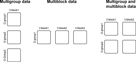
Basic multiblock structures. From left to right: different observation groups with the same variables; different variable blocks with the same observations; and both multiple observations and multiple variables

For example, the experimental setup could involve the collection of both urine and plasma samples (leading to two blocks of variables) from two groups of patients, i.e. Control, and Treated. Two repeats of the measurements before and after the treatment could offer valuable information on patient-specific effects, thus giving rise to two observations per treated patient. Moreover, additional information could be gained from the inclusion of another group of External controls, for which only the plasma sample is available. The structure of the whole dataset corresponds therefore to a 7-block arrangement as depicted in Figure 2, with the block-to-group mappings summarized in Table 1. The challenge is then to handle this type of complex data structure in a generic way. Most forms of multigroup and multiblock analysis methods can actually be considered as a combination of several single-group models evaluated either from different observations with an added constraint of sharing the same loadings over the variables, or from multiple variable blocks measured over the same set of observations. The fact that, algebraically, multigroup and multiblock analysis are the same problem is well known (Van Deun et al., 2009). The actual difference lies only at the level of data processing, i.e. how the different blocks should be centred and scaled. The components are then obtained by some low-rank approximate decomposition of the matrices, in an appropriate sense (typically the least squares of the residuals). As a consequence, these components define new directions in the data space grasping salient characteristics of multiple groups of observations and/or blocks of variables. From that point of view, the structural relations between the data matrices are equality constraints between the so-called loadings of the low-rank decompositions. Recent works have led to the development of new methods that constitute generalizations of multivariate methods to multigroup or multiblock cases (Eslami et al., 2013; Tenenhaus and Tenenhaus, 2014). The aim of the present work is to extend that rationale to arbitrary relations of shared loadings between data tables, whether between groups of observations or between blocks of variables. The proposed approach aims to model the data matrices by a set of linear models whose principal directions of covariations are shared. Depending on the multiblock or multigroup setting, this leads to a model that can be seen as a within-group analysis when the means of the variables in a given block are zeros, or unsupervised between-group analysis, when the means of variables across all connected groups are considered. Among the several different data configurations (groups or blocks), we can distinguish the most typical cases: (i) one block and one group boils down to standard PCA, (ii) multiple blocks describing a single group of observations is equivalent to CPCA (or SUM-PCA), (iii) multiple groups characterized by a single block leads to SCA-P (Van Deun et al., 2009). As the goal of the model is to provide a structured decomposition of the data network by extracting common information among groups of observations and blocks of variables, it does not attempt to explicitly disentangle common and individual sources of variability using loadings defining specific subspaces. To this aim, the reader can refer to several recently published methods potentially involving orthogonality constraints to separate joint covariations from distinct variations (Lock et al., 2013; Måge et al., 2012; Menichelli et al., 2014; Næs et al., 2013; Schouteden et al., 2013). Because NetPCA is not based on this common/distinctive information decomposition principle, the same number of components is used to summarize all the data matrices of the network. This feature can be seen as a limitation, as groups of observations and/or blocks of variables can have very different ranks, that can lead to discrepancies in the number of components needed to capture the dimensions underlying the different data matrices. However, it should be noted that NetPCA is able to grasp specific patterns of given groups of observations or blocks of variables.

Fig. 2.

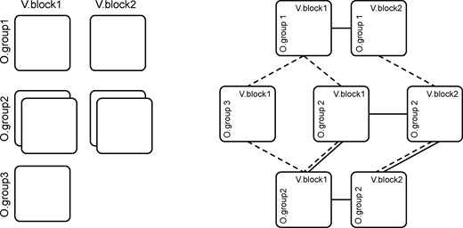
Complex data structure. Each square corresponds to a data matrix of given observations and variables. Left: dataset with two variables blocks and three observations groups, a missing block (O.group3 × V.block2) and an additional repeated measure of O.group2 for both V.block1 and V.block2. Right: corresponding network structure highlighting the links of shared loadings between variables (dotted lines) and observations (solid lines). Note that the sharing is transitive and that this structure cannot be correctly flattened into a concatenated matrix

Table 1.

Description of study exemplifying Figure 2

Data matrix b	Observables O(b)	Variables V(b)	Repeat
Control, urine	Control (O.group1)	Plasma (V.block1)	1
Control, plasma	Control (O.group1)	Urine (V.block2)	1
Treated (before), urine	Treated (O.group2)	Plasma (V.block1)	1
Treated (before), plasma	Treated (O.group2)	Urine (V.block2)	2
Treated (after), urine	Treated (O.group2)	Plasma (V.block1)	1
Treated (after), plasma	Treated (O.group2)	Urine (V.block2)	2
External, plasma	External (O.group3)	Plasma (V.block1)	1

As connection links between data matrices define the constraints of the model, other general structures of block-based data could be handled using a similar approach, such as in the case of missing blocks or tensor substructures, as shown in Figure 2. This illustrates the high versatility of the proposed approach, which makes it possible to take advantage of all available data by relying on the connections between matrices. Such a modelling strategy can therefore be applied to many situations without modification.

Missing data can arise from either the mishandling of data or, more likely, data sources that are not available for all the observation groups. This scenario is particularly common in clinical contexts and retrospective studies. Comparisons between diseased patients and healthy volunteers can be difficult because of the lack of biological information from laboratory tests that have not been performed on the entire cohort. For example, certain individuals may not be subject to particularly invasive techniques for external reasons that cannot be controlled. On the other hand, retrospective studies, by their very nature, do not make it possible to plan the experimental design that led to measurements carried out several years before. Typical solutions are either to discard all unavailable data for the whole experiment, which carries a large risk of missing important within-group structures, or to use data imputation strategies. However, this latter approach complicates the interpretation of the model scores and loadings between partially or fully available variables. Treating the whole dataset as a multiblock structure, with per-block models and connections enforced by the sharing of the loadings, overcomes these problems by allowing an interpretation of the loadings in the context of their relevant data matrices. With regard to tensor structures, longitudinal studies present another scenario where several blocks are measured for the same individuals and variables. Repeated measures on the same individual before and after some treatment or during a temporal follow-up naturally create tensorial structures. In the first case, the prevalent approach is to treat differences between individuals before and after, while considering repeated measures as statistically independent (flattening the structure), which is not strictly correct. Accounting appropriately for the links between slices of a tensor, i.e. repeats in that case, can be achieved using adapted constraints derived from the structure, as depicted in Figure 2. Due to the possibility of collecting multiple observations for the same individuals, the term observations (e.g. each particular set of measures for one individual) and observables (e.g. the individuals themselves for whom observations can be made) will be distinguished throughout this article. The low-rank decomposition of tensorial data has also been extensively studied (Bro, 1997; Carroll and Chang, 1970; De Lathauwer et al., 2000). However, the established methods, such as PARAFAC, focus on full three-way data that constitute complete cube of entries. This consideration makes sense when the structure involves a series of measurements in the third mode completely common to the variable and observation modes. While this framework is appropriate for the analysis of hyperspectral data, clinical studies and many other experimental setups will most often be similar to the case described in Figure 2. Given sets of observations/variables can indeed be associated with repeated measures, but these do not necessarily imply a logical relationship between the slices along the longitudinal axis, e.g. observations may have been made at t = 0 for groups A and B, and then follow-ups were carried out at different time points for each. For this reason, one of the main goals of this work was to develop a method able to handle completely generic relations between data matrices.

First, the notation used to describe the data network will be introduced. Then the aim and principles of the method will be explained in Section 2.1. Model outputs will be detailed with respect to interpretation, before a description of the software implementation. Finally, a case study involving multiple groups and blocks will be used to illustrate the ability of the proposed method to handle a complex data structure.

2 Materials and methods

A convenient way to describe structured data in the most general form is to define each data table b as a single matrix, $X_{ij}^b$⁠, where b denotes the matrix, while indices i and j correspond to the rows and columns of the data matrices, associated respectively with observations and variables. The loadings, in turn, will not correspond to a specific matrix but to the observable/variable subsets. These are determined by the relations between the matrices, creating two networks of links, i.e. one for observables and one for variables. The component connected to a given matrix b under each network will be its observable group O(b) or variable block V(b), respectively. A detailed description of the notation is available in Section S1.1 of Supplementary Material.

2.1 Theory

The proposed approach aims to model the ensemble of matrices $X_{ij}^b$ by a set of linear models whose principal directions are shared between data tables with matching observable or variable subsets. Each observable has its own mapping $U_i^{O(b)}$ in the subspace defined by the loadings, while $W_j^{V(b)}$ corresponds to the mapping of the variables. The approximation of each table $X_{ij}^b$ using N components is summarized by the following equation:

$$X_{ij}^b\sim \sum _{\alpha =1}^{N_{\text{comp}}}{}^{\alpha }{\sigma }^b{·}^{\alpha }{U}_i^{O(b)}{·}^{\alpha }{W}_j^{V(b)}.$$

(1)

where the similarity is to be understood up to residual terms to be minimized with respect to some goal function.

The values of ${}^{\alpha }{\sigma }^b$ hold what is essentially the (square root) variance associated to the matrix b on the αth component. ${}^{\alpha }{U}_i^{O(b)}$ and ${}^{\alpha }{W}_j^{V(b)}$ hold the loadings for the matrix’s observables O(b) and variables V(b), respectively. The key point is that the sharing of the loadings between data tables with the same groups and/or blocks is enforced by the fact that they are the same mathematical objects.

In this context, it is important to distinguish between the usual concept of scores for the observations (the projections of the data tables onto the variable loadings) and the set of loadings ${}^{\alpha }{U}_i^o$ for the observables. The main difference is that the observable loadings represent a principal direction in the observable space and are therefore shared by all blocks having the same observable group, while scores are computed per block. For instance, two data tables corresponding to the same variables measured for the same patients will both belong to the same observable groups and variable blocks (and therefore have the same set of loadings), but the scores resulting from the projection of each dat matrix onto the variable loadings will be different, because they are related to distinct subsets of observations.

The proposed goal function to estimate the model parameters involves finding a minimum of the total squared error between the data tables and the model, potentially weighing each matrix by a fit weight ω_b,

$$\sum _b{\omega }_b^2\sum _i\sum _j{\left({\sigma }^b{U}_i^{O(b)}{W}_j^{V(b)}-X_{ij}^b\right)}^2,$$

(2)

with the constraint that the loadings U and W must have unit Euclidean norm over each group of observables or variables. The minimization target is the same PCA would require matrix-by-matrix, with the additional constraint that the loadings are shared between them. A detailed description of these aspects is available in Section S1.2 of Supplementary Material. Finding the global minimum of this function with these restrictions is not algebraically trivial, as the same variables appear in multiple terms. However, considering the restriction to a function of only either the U or W loadings, this goal is a quadratic positive-definite form, and the minimization problem becomes a largest eigenvalue problem. Starting with an equal guess of the importance of each observation,

$$U_i^o=1/\sqrt{N(o)},$$

(3)

where N(o) is the number of observables in group o, an alternating least squares strategy is used to compute approximations to W and U by fixing one term to solve the other using a two-step iterative procedure. This procedure can be shown to converge, with more details provided in Section S1.3 of Supplementary Material. This alternating least squares minimum may not necessarily be a global minimum, but it still provides components explaining a large fraction of the variability in the data. Instead, the algorithm provides a deterministic solution for each dataset, without random initialization or computational steps.

The fit weights ω_b are introduced to adequately combine data coming from sets with very different cardinality. An example can be a set of a few variables originating from targeted analyses carried out on a limited subset of metabolites of biological interest, and another block of untargeted analyses with several orders of magnitude more data. In concatenated PCA, as the same a priori chance to contribute to the model is allocated to a variable from one block or the other, the targeted data loadings will most likely pick up only spurious correlations with the untargeted data or have close to zero loadings. Multiblock approaches in general already solve this problem to a large degree by allowing the small data to contribute with its own projection space, where it must find a principal direction of correlation with the rest of the data. However, without interblock normalization, the untargeted data of the example will determine its own principal direction with nearly no influence from the targeted. The choice of normalization depends on the scaling and type of data. For unit-variance scaled data, we recommend weighing the fit with

$${\omega }_b=\frac{1}{\sqrt{N(O(b))·N(V(b))}},$$

(4)

which gives each block the same amount of influence on the global fit. Details about this normalization, and alternatives such as Pareto scaling also frequently used in metabolomics, can be found in Section S1.6 of Supplementary Material.

As mentioned before, scores are projections of the data onto the loading subspace. In PCA, the orthogonality of the loadings between different components means that scores have a particularly simple form, as they are the principal directions in the observation space. However, two problems arise in the case of a network of interconnected data matrices. First, loadings will generally be close to but not completely orthogonal. Second, the principal directions given by the loadings are shared by all blocks having the same observables. Yet groups sharing observables but with different observations should have different scores. The simplest solution is to actually go back to the initial meaning of the scores ${}^{\alpha }{S}_i^b$⁠, and project the data onto the loadings:

$${}^{\alpha }{S}_i^b:=\sum _j{X}_{ij}^b{·}^{\alpha }{W}_j^{V(b)}.$$

(5)

This allows multiblock scores to be considered as representing the projection of a set of observables over multiple variable blocks, ${}^{\alpha }{S}_i^{\{b_1,\dots ,b_n\}}$⁠, as the average of the scores. More details about the estimation of the model parameters are presented in Section S1.4 of Supplementary Material. The described steps produce a set of parameters for a single component of the model. Further components can be computed by the usual approach of deflation. The latter is described in Section S1.5 of Supplementary Material. Figure 3 provides a summary of the algorithm, while a detailed description of the network model is provided as Supplementary Material, including the notation for all the objects used in the construction, the presentation of the building blocks of the model, the minimization problem and the iterative algorithm generating its solution, and its convergence.

Fig. 3.

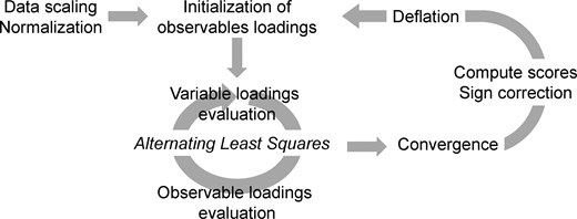
Algorithm summary, including initialization, alternating least squares procedure, score projection, sign fixing and deflation

2.2 Model interpretation

The interpretation of most multivariate linear models involves an evaluation of both the relevance of each variable (represented by their loadings) and the overall variability of each observation within the model (represented by their scores). It usually begins with finding some trend in the score plot by inspecting the distribution of the observations in the lower-dimensional component subspace, and observing meaningful groupings (e.g. separation of experimental groups). As introduced in Section 2.1, NetPCA scores should be computed by projecting the data over the direction in the variable space specified by the loadings. Variables that are relevant for this component are then highlighted from the loadings, assuming them to be pertinent to explain the effect. The main advantage of linear models is to provide a straightforward way to interpret the influence of each variable through the loadings. Our approach is based on the same principle, and each set of loadings ${}^{\alpha }{W}_j^v$ provides the usual interpretation of the relevance on the global model of the variable j belonging to the variable block v. Moreover, additional information can be extracted from the model, because groups of observations and/or blocks of variables are treated as natural units of information that may hold different direction and magnitude of variability. It is to be noted that sign ambiguity can lead to flipped axes, that constitute an issue when combining loadings from different groups. The sign is thus chosen so that a positive score would be associated with an observation where its variables on average are higher than the mean. The interested reader can refer to Section S2.3 of Supplementary Material for more details on this procedure. Moreover, it may be the case that multiple groups are separated at each side of a certain component but that the main variables affecting them are not the same. Explicitly taking into account the group structure of the observables makes it possible to assess the relevance of a given variable for a specific group. As a consequence, ordering variables by their influence on the groups of interest instead of their overall loadings constitutes an effective way to interpret the model. As several groups of observations need to be represented by the same observable loading, not all of them will be fitted by this loading to the same degree. This is the critical part of the between-group interpretation of the variable importance since it precisely captures the appropriateness of the given loading for a specific group. We define this variable influence on a group as the relative explained variability lost when setting its corresponding loading to zero in the given group and component. This notion of variable influence has a straightforward interpretation and naturally takes into account the possible effects of the lack of orthogonality of the loadings. By construction, it is also an additive quantity, and the total explained variance of the model is the sum of the importance of each of the variables. Due to the additivity, it is also possible to rank variables by their total influence over some specific subsets of groups. Comparing the influence of variables belonging to different variable blocks is also meaningful, as opposed to directly comparing their loadings. Details about the interpretation of block scores, as well as variable and block influences can be found in Sections S2.1 and S2.2 of Supplementary Material, respectively.

2.3 Software implementation

The algorithm has been implemented as a Python 3.0 package with dependencies on NumPy (Oliphant, 2006) for numerical computations and Plotly (Plotly Technologies Inc., 2019) for model visualization. The library includes modules to load data from CSV/XLSX files and configure the network relationships between the data matrices, to compute the model and to generate an interactive HTML report including the block structure, selectable score plots, variable loadings and influences, variable boxplots and the contributions of each variable to the model. Additionally, a Jupyter notebook example of use is provided. A short demonstration of the package with an illustrative screenshot of the summary offered by this report is available as Supplementary Material, and can be found at gitlab.unige.ch/Julien.Boccard/netpca.

3 Results

A real case study involving metabolomic data collected from a cohort of patients suffering from chronic kidney disease (CKD) was chosen to illustrate the qualities of the proposed algorithm (Gagnebin et al., 2018). The aim of this study was the untargeted investigation of metabolic alterations according to the progression of the disease, and the effect of hemodialysis. Blood samples were obtained from a set of 56 control patients, 69 in the intermediate CKD stage (levels 3b–4 according to the glomerular filtration rate criterion) and 35 in the advanced CKD stage (level 5, i.e. close to renal failure). These 35 advanced CKD patients were also studied after blood dialysis, to understand its impact and evaluate its ability to bring the metabolome closer to the healthy situation. The corresponding observable groups in our model were the Control (CTRL), Intermediate CKD (ICKD) and Advanced CKD before (ACKD-0) and after dialysis (ACKD-1).

The samples were analysed with four LC-MS techniques (reversed phase LC with ESI+/-, amide-based hydrophilic interaction LC with ESI+ and zwitterionic-based hydrophilic interaction LC with ESI-), providing a total of 33’459 analytical features after data preprocessing, filtering and normalization based on QC samples (Broadhurst et al., 2018; Pezzatti et al., 2020). Of these, 344 could be related to level 1 annotations based on mass and retention time matching the standards measured in-house. Notably, 4’286 additional features were found to have mass matching entries in the KEGG database (Aoki and Kanehisa, 2005). The block structure is summarized in Figure 4. A special focus is placed on the methodological aspects of the proposed model, particularly with regards to the connections between matrices, rather than a biological interpretation of the data, which was already considered in (Gagnebin et al., 2019).

Fig. 4.

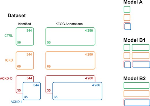
CKD application data structure, illustrating the complexity of modern multigroup and multiblock datasets. Different possible models for analysis are shown on the right. Colour code: green CTRL, orange ICKD, red ACKD-0, blue ACKD-1

3.1 Network models based on annotation levels

Several modelling strategies can be considered to handle this type of data structure and gain biological insights to describe a given phenomenon. The first model (Model A) is designed to focus only on well-characterized biochemical information based on level 1 metabolic annotations, i.e. formally identified metabolites. The second approach (Models B) consists in integrating the complementary information offered by the automatic annotation of a large number of potential metabolites. This second block of variables is obtained by comparing the analytical features with metabolic database entries (here KEGG). It should be noted that the structure of the blocks of variables is preserved in Model B1, while horizontal concatenation of all the available data is carried out in Model B2. The latter approach is often used because of its ease of implementation with existing multivariate approaches (e.g. PCA or SCA).

First, let consider a model using only the 344 level 1 annotations, corresponding to Model A in Figure 4. The score plot is shown in Figure 5 top. The first component clearly discriminates between the CTRL group and the affected patients, and follows the progression of the disease. Most of the variability is taken by advanced (ACKD-0) patients, which is not surprising, since renal dysfunction is associated with decreased glomerular filtration, leading to an increase of the concentration of many metabolites. Interestingly, dialysed (ACKD-1) patients return to the position of the intermediate (ICKD) group after dialysis along the first component, but another effect occurs along the second component, separating ACKD-1 from the other groups.

Fig. 5.

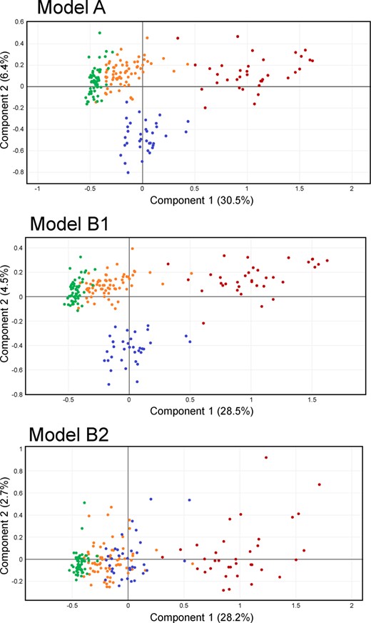
CKD Model A, B1 and B2 scores. Colour code: green CTRL, orange ICKD, red ACKD-0, blue ACKD-1

As mentioned in the introduction, one of the main reasons to run untargeted metabolomics analyses is to find potentially interesting features that are not included in the relatively limited database of standards available in a laboratory. A looser process of annotation (based only on mass matching against the KEGG database in this case) leads to considerably more annotated features than the more reliable level 1 annotation, and many of these new candidates may be either analytical noise, or otherwise biologically irrelevant. This becomes manifest when they are included in the model in the way described in Figure 4 as Model B2, i.e. by simply concatenating these additional variables with properly identified metabolites, as would be done in most metabolomic studies. Unsurprisingly, this has the effect of generating the score plot of Figure 5 bottom. Because there are many more variables originating from simple mass matches than from level 1 annotations, and because a large fraction of them are probably not relevant, the effect that separated ACKD-0 and ACKD-1 patients is lost in the noise. This issue is explicitly taken care of when performing an analysis following the full structure of Model B1 from Figure 4. The resulting score plot, depicted in Figure 5 middle, shows again the relevant separation between those two states of ACKD patients. At the same time, the underlying model offers a potent way to search among the putative metabolites from the KEGG block to find additional relevant signals that are related to the observed effects.

3.2 Variable influences

Accounting explicitly for the separation into blocks in the variable direction helps to maintain the interpretability of the model. Yet there is also interest in grouping along the observation direction. The relevance of variables in a per-group sense can be investigated using the variable influences. This parameter allows evaluating the contribution of each variable to describe the variability of a given group of observations in an objective manner. Although biological details are not the focus, these influence distributions offer information about metabolite patterns. For example, it is clear that most of the variability related to the first component is generated by ACKD-0 patients. However, for diagnosis purposes, one could be interested in the compounds affecting particularly the separation of the healthy (CTRL) and mild disease (ICKD) patients on the first component. The main variables explaining their variability are not necessarily the same as those for ACKD-0. This can be easily investigated by sorting the variable influences by their combined effect on these two specific groups.

Figure 6 top shows the influence distribution of level 1 annotations, sorted according to this criterion. Consistent with prior knowledge of CKD, more variables are increased than decreased in the direction linked to ACKD-0, since renal dysfunction affects glomerular filtration. On the other hand, the negative direction of metabolites that are more abundant in the CTRL and ICKD groups, is associated with a few clearly prominent variables (Gagnebin et al., 2019).

Fig. 6.

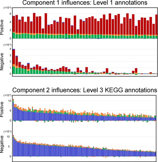
CKD Model B1. Component 1: distribution of the first 50 variable influences, separated by loading sign, sorted by CTRL (green) and ICKD (orange). Component 2: first 150 variable influences, separated by loading sign, sorted by ACKD-1 (blue)

Interestingly, sorting variables according to their relevance for CTRL and ICKD is noticeably not the same as sorting by global influence (the whole bar height) or by the absolute value of their loading. This result highlights the fact that the observation-wise data structure provides a more detailed understanding of the importance of each variable.

Figure 6 bottom shows the influences on the second component for the variables obtained from KEGG mass matches, sorted by the relevant block, i.e. ACKD-1 patients. Such an ordering could be used for instance to select the most influential variables to conduct further experiments (such as MS/MS spectrum matching). Additionally, the bar plots display a characteristic feature of the variable influences, namely that some of them are negative. This should not be confused with a positive or negative loading ${}^{\alpha }{W}_j^v$⁠, but rather reveals that the contribution of certain variables may actually increase the total residual error in a given data table. Indeed, a variable loading whose presence in the model slightly increases the error in one matrix is an acceptable trade-off for an important decrease in every other data matrices. It should also be noted that usual PCA inherently has these kinds of trade-offs, as it minimizes the total residual error between the data and its reconstruction. The difference lies in the fact that using a block structure offers a straightforward way to assess which blocks are affected, potentially in a negative way as far as the reconstruction is concerned, and by which variables. For instance, if the highest loading corresponds to a variable that has an important negative variable influence on one of the data tables, a warning is given indicating that additional attention needs to be paid to its interpretation.

Finally, Figure 7 shows the influences summed over all variables on each block for both components. Such heatmaps provide a quick way to see the relative contributions of each variable subset to the decomposition.

Fig. 7.

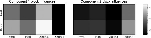
CKD Model B1 block influences. Left: first component. Right: second component

3.3 Interactive visualization

Complex multiblock structures can be inspected and understood from a wide variety of viewpoints and there is a plethora of combinations of relevant blocks, variables, components and metrics to consider. Traditional static visualization approaches are limited by their need to choose between all possible permutations of the parameters, or leaving out what is considered as less relevant information. To avoid this, the proposed implementation includes the automatic generation of an interactive HTML5 report, without any more requirements than a standard browser to open it and leaving all the interactivity to the user: selected blocks, components, filters, synchronized information and tooltips. A screenshot of this report, as generated for the CKD dataset, can be seen in Figure 8.

Fig. 8.

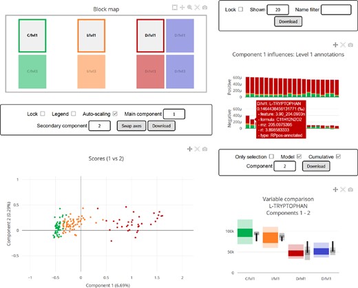
Screenshot of the interactive HTML report generated by the Python library

3.4 Concluding remarks

The proposed NetPCA method offers a versatile strategy to investigate complex multigroup and multiblock structures with linear models, motivated in particular by missing block or tensorial/longitudinal experimental designs. The proposed algorithm provides an adaptable data decomposition guaranteed to converge to a deterministic minimum of the summed residual square error, and introduces several useful metrics to assess the influence of variables and blocks on both the overall model and the particular data tables. As a case study, the model was applied to a real-world metabolomic dataset collected from patients enrolled in a CKD clinical study. Accounting for the multigroup and multiblock structure was shown to be crucial to appropriately investigate the data. On the one hand, model parameters provided relevant feedback on each group’s influence on the global model. On the other hand, the investigation of an additional block of variables with a lower degree of annotation confidence, a larger dataset size and higher noise, was made possible by assessing the influence of each variable on the different experimental groups.

Acknowledgements

The authors thank Belén Ponte, Julian Pezzatti and Pierre Lescuyer for providing the CKD dataset, and for useful discussions.

Funding

This work was supported by the Swiss National Science Foundation [31003A_166658].

Conflict of Interest: none declared.