


Abstract
3D neuron segmentation is a key step for the neuron digital reconstruction, which is essential for exploring brain circuits and understanding brain functions. However, the fine line-shaped nerve fibers of neuron could spread in a large region, which brings great computational cost to the neuron segmentation. Meanwhile, the strong noises and disconnected nerve fibers bring great challenges to the task.
In this article, we propose a 3D wavelet and deep learning-based 3D neuron segmentation method. The neuronal image is first partitioned into neuronal cubes to simplify the segmentation task. Then, we design 3D WaveUNet, the first 3D wavelet integrated encoder–decoder network, to segment the nerve fibers in the cubes; the wavelets could assist the deep networks in suppressing data noises and connecting the broken fibers. We also produce a Neuronal Cube Dataset (NeuCuDa) using the biggest available annotated neuronal image dataset, BigNeuron, to train 3D WaveUNet. Finally, the nerve fibers segmented in cubes are assembled to generate the complete neuron, which is digitally reconstructed using an available automatic tracing algorithm. The experimental results show that our neuron segmentation method could completely extract the target neuron in noisy neuronal images. The integrated 3D wavelets can efficiently improve the performance of 3D neuron segmentation and reconstruction.
The data and codes for this work are available at https://github.com/LiQiufu/3D-WaveUNet.
Supplementary data are available at Bioinformatics online.
1 Introduction
Neuron reconstruction aims to establish a digital model of the neuron morphology structure by tracing nerve fibers in neuronal image, which is of great significance to explore the brain microstructure and understand brain functions. 3D microscopic optical imaging technology, such as Micro-Optical Sectioning Tomography (MOST) (Li et al., 2010), has established a foundation for the brain neuron reconstruction. Tens of automatic or semi-automatic tracing algorithms (Liu et al., 2018b; Quan et al., 2016; Xiao and Peng, 2013) have been developed to reconstruct the neurons in optical images. However, the low signal-to-noise ratio and disconnected nerve fibers are usually big challenges to these algorithms, as Figure 1 shows.
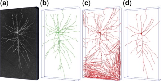
(a) A noisy neuronal image with size of (z-y-x), containing a complete neuron. (b) The manual reconstruction of the neuron. (c) An automatic reconstruction which incorrectly takes background noises as nerve fibers. (d) Another automatic reconstruction which overlooks the weak nerve fibers
A natural way to improve the performance of existing neuron tracing algorithms is to extract the complete neuron from the noisy image first and then automatically reconstruct it. Deep learning, which achieves excellent results in many fields, has also been applied into 3D neuron segmentation (Huang et al., 2020; Jiang et al., 2021; Klinghoffer et al., 2020; Li et al., 2017; Li and Shen, 2020). As nerve fibers can spread in a very large brain region, a large neuronal image has to be processed for segmenting the complete neuron, which leads to great computational cost for the deep networks-based 3D neuron segmentation. In addition, the recent researches (Li et al., 2020; Zhang, 2019; Zou et al., 2020) show that the sampling operations used in the deep networks result in aliasing effects, which lead to noise propagation and break the basic object structures. Due to the amount of noises available in the neuronal image and the neuron’s fine line-shaped structure, 3D neuron segmentation is more sensitive to these aliasing effects. Therefore, the current 3D deep network-based segmentation methods might not work well for the 3D neurons with fine line-shaped structure in the noisy neuronal images.
1.1 Related works
1.1.1 Neuron reconstruction
The recent brain imaging technologies, including Micro-Optical Sectioning Tomography (MOST) (Li et al., 2010), fluorescence MOST (fMOST) (Gong et al., 2013), CLARITY (Chung et al., 2013; Chung and Deisseroth, 2013), Magnified Analysis of the Proteome (MAP) (Ku et al., 2016) and Stabilization under Harsh conditions via Intramolecular Epoxide Linkages to prevent Degradation (SHIELD) (Park et al., 2019), etc., establish the foundation for neuron reconstruction of animal brain.
Various 3D data visualization software, such as Vaa3D (Peng et al., 2010b), NeuroBlocks (Ai-Awami et al., 2016), ManSegTool (Magliaro et al., 2017), TeraVR (Wang et al., 2019b), etc., have been developed to show the complex arborization fibers in neuronal images and assist the experienced technicians in tracing neurons. BigNeuron project (Peng et al., 2015), initiated by Peng et al., releases hundreds of optical neuronal images and their high precision reconstructions traced by experienced experts. More than digitally reconstructed neurons are released on NeuroMorpho.Org (Ascoli et al., 2007), while the corresponding neuronal images are not available.
It is impossible to manually reconstruct the millions of neurons in the whole brain image, so various automatic neuron tracing algorithms have been designed. The BigNeuron project (Peng et al., 2015) collects the tens of these algorithms, such as SnakeTracing (Wang et al., 2011), All-Path-Pruning (APP) (Peng et al., 2011), APP2 (Xiao and Peng, 2013), NeuroGPSTree (Quan et al., 2016), Rivulet (Liu et al., 2016), Rivulet2 (Liu et al., 2018b), etc., and integrates them into the Vaa3D software (Peng et al., 2010b). Generally, these algorithms mathematically model neuron morphology and trace nerve fibers based on graph theory. However, they would either classify background noise as nerve fibers or miss lots of nerve fibers, as Figure 1 shows. In other words, while the tracing algorithms are sensitive to image quality, the existing neuronal imaging technologies are usually associated with low signal-to-noise ratio.
1.1.2 Neuron segmentation
Segmenting the neuron before reconstruction is an effective approach to improve the performance of neuron tracing algorithms. Inspired by the superior performance in computer vision, pattern recognition and natural language processing, etc., deep learning has also been introduced into the 3D neuron segmentation (Huang et al., 2020; Jiang et al., 2021; Klinghoffer et al., 2020; Li et al., 2017; Li and Shen, 2020; Wang et al., 2019a). The first 3D residual deep network for neuron segmentation is proposed in (Li et al., 2017). The authors improve their method by applying multi-scale kernels and 3D U-Net (Wang et al., 2019a). Because they take as input the original neuronal image, these deep networks require high computational cost. Li and Shen (2020) designed 3D U-Net Plus to separate the target neuron from its surrounding nerve fibers. As 3D U-Net Plus is trained and evaluated on the neuronal images with size of , the small nerve fibers may disappear during the image down-sampling. The above deep network-based neuron segmentation methods are not suitable for neurons with long-distance fibers. Using ray-shooting model, Jiang et al. (2021) design dual channel Bidirectional Long Short-Term Memory (BLSTM) for 3D neuronal image segmentation. The authors extract nerve fibers from the 2D neuronal image slice-by-slice, which does not utilize the relevance between the nerve data in the neighboring 2D neuronal slices. To utilize the unlabeled 3D neuronal data, self-supervised and weakly supervised 3D neurons segmentation methods are studied (Huang et al., 2020; Klinghoffer et al., 2020). In all of these works, the BigNeuron (Peng et al., 2015) neuronal images are taken to test their methods.
1.1.3 The aliasing effects in deep networks
The recent studies (Li et al., 2020; Zhang, 2019; Zou et al., 2020) reveal the aliasing effects in the deep learning, which are introduced by the commonly used sampling operations in the deep networks. The aliasing effects result in noise accumulation and break the basic object structure in deep networks, which are very harmful to the 3D neuron segmentation in noisy images.
To suppress the aliasing among the low-frequency and high-frequency components of the data in deep networks, Richard (Zhang, 2019) designs Anti-aliased CNNs by applying low-pass filters before the down-sampling in common Convolutional Neural Networks (CNNs). Zou et al. (2020) propose an adaptive content-aware low-pass filtering layer to adapt the varying frequencies in different locations and feature channels. These works only consider the low-frequency component of input data, which cannot extract and utilize the data details represented by the high-frequency components. Li et al. (2020) integrated discrete wavelet transforms (DWT) into deep networks to separate the components of data in different frequency intervals. They illustrate the usefulness of wavelet transforms in assisting deep networks in extracting robust features, keeping basic object structure and recovering data details.
The above works suppress the aliasing effects in 2D deep networks, while they are not available to 3D deep networks for the 3D neuron segmentation. The 3D neuronal images contain a lot of noises and the neurons are line-shaped, which are more easily broken by the aliasing effecting in 3D deep networks. Inspired by Li et al. (2020), we try to introduce 3D wavelet transforms into deep learning to suppress the aliasing effects in 3D deep networks. In the previous works, such as Shi and Pun (2017); Yang et al. (2019), and so on, 3D wavelet have been developed as pre-processing or post-processing tools for deep networks. Shi and Pun (2017) apply 3D wavelet to decompose hyperspectral image into various components wavelet domain, and apply 3D CNNs on the components to extract features for the hyperspectral image classification. Yang et al. (2019), using 3D CNNs, predicted the coefficients of hyperspectral image in 3D wavelet domain, to reconstruct hyperspectral image with super-resolution. In these works, only Haar wavelet was applied to evaluate their methods. Because they do not integrate 3D wavelets into 3D deep networks, they cannot suppress the aliasing effects in 3D deep networks. In contrary, in this article, we rewrite 3D wavelet transform as network layers in PyTorch, which are applicable to various discrete wavelets (such as Haar, Cohen and Daubechies wavelets), and could be flexibly integrated into 3D deep networks to suppress the aliasing effects in networks.
In this article, we will rewrite 3D DWT/IDWT as general network layers, and design 3D wavelet integrated encoder–decoder networks, to improve the 3D neuron segmentation and reconstruction in noisy images.
1.2 Contributions
In this article, to completely segment the neuron and efficiently improve its reconstruction, we present a 3D wavelet and deep learning-based 3D neuron segmentation method. First, to simplify the task, we partition the neuronal image into small cubes. Then, we design a 3D wavelet integrated encoder–decoder network (3D WaveUNet) to segment the nerve fibers in the cubes. As far as we know, 3D WaveUNet is the first 3D wavelet integrated deep network. In 3D WaveUNet, 3D Discrete Wavelet Transform (3D DWT) and 3D Inverse DWT (3D IDWT) are applied to down-sample and up-sample 3D neuronal data. While 3D DWT help the encoders in maintaining the fine structure of neurons and suppressing the noise propagation, 3D IDWT could recover the neuron details in the decoders. In addition, based on the biggest available annotated neuronal image dataset, BigNeuron (Peng et al., 2015), we produce a Neuronal Cube Dataset (NeuCuDa) to train and evaluate the 3D WaveUNet. Finally, we assemble the nerve fibers segmented in cubes according to the cube locations to get the complete segmented neuron, and reconstruct it using the existing automatic tracing algorithms, such as All-Path Pruning 2.0 (APP2) (Xiao and Peng, 2013). In summary:
We propose a 3D wavelet and deep learning-based 3D neuron segmentation method, to segment neurons in large size 3D neuronal images.
We rewrite 3D DWT/IDWT as general network layers, and design 3D WaveUNet by applying 3D DWT and IDWT as the sampling operations in 3D encoder–decoder network, which is the first 3D wavelet integrated deep network.
We produce a neuronal cube dataset, NeuCuDa, to train and evaluate the 3D WaveUNet. Experimental results show that 3D WaveUNet efficiently improve the performance of 3D neuron segmentation and reconstruction in the noisy images.
2 Materials and methods
2.1 The method pipeline
The pipeline of our 3D neuron segmentation method is illustrated in Figure 2 and summarized as below:
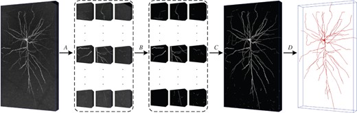
The pipeline of our 3D neuron segmentation method. A: Partition. B: Segmentation. C: Assembling. D: Reconstruction
Partition. The neurons with long-distance nerve fibers could spread in a large brain region, which result in high computational cost for the 3D neuron segmentation in the images with large size. Therefore, the neuronal image is partitioned into small cubes to simplify the segmentation task. We set the z–y–x-size (depth–height–width) of the cubes as (The typical voxel resolution is for brain imaging technologies, such as MOST.), which is a compromise between the connectivity of nerve fibers in the neuronal cubes and the computational complexity of the following segmentation.
Segmentation. Using the well-trained 3D WaveUNet, we segment the nerve fibers in the cubes. The 3D WaveUNet is an encoder–decoder network integrated with 3D wavelet, which are trained on the neuronal cube dataset, NeuCuDa. The network architecture and NeuCuDa are described in Sections 2.2 and 2.3, respectively.
Assembling. According to the cube locations in the neuronal image, we assemble the segmented nerve fibers to complete the 3D neuron segmentation.
Reconstruction. Based on segmented neuronal image, we reconstruct the neuron using APP2 (Xiao and Peng, 2013) algorithm. Considering its low computational complexity, we choose APP2 as the benchmark algorithm in this article.
2.2 3D WaveUNet
The aliasing effects could significantly affect the performance of deep network-based 3D neuron segmentation, due to the fine line-shaped structure of nerve fibers and interference of noises. To suppress the aliasing effects in the 3D deep networks, we design 3D wavelet integrated encoder–decoder network (3D WaveUNet), the first 3D wavelet integrated deep network, for 3D neuron segmentation.
In current, encoder–decoder networks, such as U-Net and 3D U-Net, are widely used in medical image segmentation (Li and Shen, 2020; Ronneberger et al., 2015). Although ResNets (He et al., 2016) and Transformer (Dosovitskiy et al., 2020; Touvron et al., 2020) are hot-spots in the image vision, they are hardly applied in medical image processing. Because ResNets and Transformer are pretrained using a large dataset (such as ImageNet) before they are taken as backbones in the deep networks for image segmentation, and, for 3D medical image processing, it is very hard to collect such large dataset. The proposed 3D DWT and IDWT layers are natural substitutes for the down-sampling and up-sampling operations in encoder and decoder of 3D U-Net. Therefore, we take 3D U-Net as the basic architecture, to evaluate the proposed 3D DWT/IDWT layers in 3D neuron segmentation.
2.2.1 3D DWT/IDWT layers
Wavelets (Daubechies, 1992) are powerful analysis tools used in the fields of data denoising (Donoho, 1995; Donoho and Johnstone, 1994), image compression (Bahce and Bayazit, 2020; Kim and Pearlman, 1997; Wu et al., 2009), etc., and 2D wavelets have been introduced into deep learning (Duan et al., 2017; Guan et al., 2019; Huang et al., 2017; Liu et al., 2018a, 2020a,b; Shi and Pun, 2017; Williams and Li, 2018; Yang et al., 2019; Yoo et al., 2019). Alike 2D wavelets in deep learning, 3D wavelets are applied as pre-processing or post-processing tools in deep networks. Shi and Pun (2017) applied 3D wavelet to decompose hyperspectral image into various components wavelet domain, and extract features from the components using 3D CNNs to classify the hyperspectral image. Yang et al. (2019) predicted the coefficients of hyperspectral image in 3D wavelet domain using 3D CNNs, to reconstruct hyperspectral image with super-resolution. These works do not apply 3D wavelets into the design of 3D deep networks, cannot exploit the efficiency of wavelets to process the internal 3D feature maps in deep networks.
Therefore, d, m, n are usually even numbers.
Equations (1) and (3) present the forward propagations of 3D DWT and IDWT, where the naive down-sampling and up-sampling operations are explained in Supplementary Material (Supplementary Section S.2). It is onerous to deduce the gradients for the backward propagations from these expressions. Fortunately, the modern deep learning framework PyTorch (Paszke et al., 2017) could automatically deduce the gradients for tensor arithmetics. We have rewritten 3D DWT and IDWT as general network layers in PyTorch, which will be publicly available for other researchers. One can flexibly design end-to-end 3D wavelet integrated deep networks using these layers.
For the noisy neuronal cube , the random noise mostly shows up in its high-frequency components, while the basic nerve fiber structure is presented by the low-frequency one. Therefore, 3D DWT and IDWT could be used to denoise the neuronal cube while maintaining the structure of nerve fiber at the same time. DWT halves the size of the neuronal data, and IDWT recovers it, which are good substitutes for the commonly used sampling operations in the 3D deep networks. They could be used to reduce the aliasing effects in the 3D deep networks, and improve the performance of 3D neuron segmentation and reconstruction. Figure 3 compares the results of 3D DWT/IDWT and max-pooling/max-unpooling on a neuronal cube.
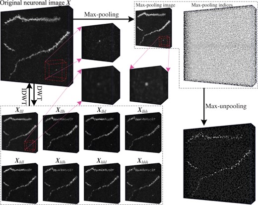
The comparison of 3D max-pooling/max-unpooling and 3D DWT/IDWT. Max-pooling would magnify the noise in the neuronal data, while noise in the low-frequency component is suppressed by 3D DWT, as the three enlarged regions show. When max-unpooling recovers the cube size, it normally breaks the nerve fibers. In contrast, IDWT could completely recover the neuronal data using the components of DWT decomposition
2.2.2 The architecture of 3D WaveUNets
In this section, we design 3D WaveUNet using 3D DWT and IDWT to increase neuron segmentation performance for better reconstruction.
As Figure 4 shows, the encoder–decoder architecture could be decomposed into several nested dual structures with a bottom block. The dual structure consists of forward process and reverse process connected via a branch path. While the forward process contains a serial of 3D convolutions followed by a down-sampling operation, the reverse process is an up-sampling operation followed by a number of 3D convolutions. The reverse process up-samples the feature maps, and exploits the data transmitted from the forward process via the branch path. The bottom block is variant in different encoder–decoder architectures. 3D U-Net (Ronneberger et al., 2015) takes a convolution block as the bottom block, while 3D U-Net Plus (Li and Shen, 2020) uses a 3D ASPP (Chen et al., 2018). We denote the all connected forward processes and reverse processes, together with the bottom block, as main path, and denote the data flowing through it as mainstream.
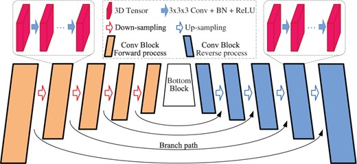
The encoder–decoder architecture
Figure 5 shows the 3D versions of dual structures used in previous encoder–decoder networks (Badrinarayanan et al., 2017; Chen et al., 2018; Çiçek et al., 2016; Li and Shen, 2020; Ronneberger et al., 2015). DS-PU, Dual Structure with max-Pooling and max-Unpooling, is a 3D version of dual structure used in SegNet (Badrinarayanan et al., 2017). As Figure 5a shows, DS-PU applies max-pooling in its forward process to reduce the feature map resolution and transmits the pooling indices to the reverse process for feature map up-sampling via max-unpooling. However, the max-pooling operation would accumulate the data noise, and the max-unpooling cannot restore the lost details, as Figure 3 shows. Figure 5b shows DS-PDc, Dual Structure with max-Pooling and Deconvolution, used in 3D U-Net (Çiçek et al., 2016) and 3D U-Net Plus (Li and Shen, 2020). While DS-PDc applies the max-pooling for the down-sampling in its forward process, it uses deconvolution for the up-sampling in the reverse process. DS-PDc copies the feature maps from its forward process to reverse process via the branch path, then concatenates it with the up-sampled feature map in reverse process to recover the low-level information in mainstream. DS-ScIn, shown in Figure 5c, has the same structure with DS-PDc, while it applies Strided-convolution and linear Interpolation for down-sampling and up-sampling, respectively. In DS-PDc and DS-ScIn, the data tensor injected from their forward processes to reverse processes contains redundant information including noises, which could interfere with 3D neuron segmentation.
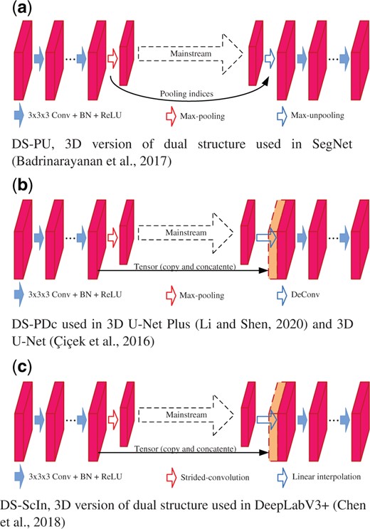
The 3D versions of the commonly used dual structures
We design four 3D Wavelet-based Dual Structure (WADS) by replacing the sampling operations with 3D DWT/IDWT, as Figure 6 shows. In comparison, WADS-DDc (Fig. 6a) and WADS-DIn (Fig. 6b) are designed by replacing the down-sampling operations in DS-PDc and DS-ScIn with 3D DWT, respectively. In their forward processes, while the feature map is decomposed by 3D DWT into eight components, only the low-frequency one is kept to extract the robust high-level features, and the seven high-frequency components are abandoned. WADS-DI (Fig. 6c) and WADS-DIDn (Fig. 6d) apply 3D DWT and 3D IDWT for down-sampling and up-sampling in their forward and reverse processes, respectively. In the forward process, while feature map is decomposed by 3D DWT, the low-frequency component is kept to extract the robust high-level features, and the seven high-frequency components are transmitted, via the branch path, to reverse process for feature map up-sampling in 3D IDWT. WADS-DIDn utilizes a denoising block to filter the high-frequency components; the denoising block is implemented using hard shrinkage, which is shown in Supplementary Material.
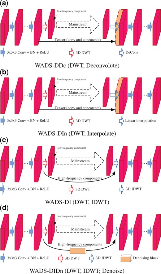
The 3D wavelet integrated dual structures (WADS)
Using the seven dual structures, we design seven 3D encoder–decoder networks, including four wavelet integrated ones (3D WaveUNets), for neuron segmentation. They are named as 3D U-Net(x), and 3D WaveUNet(y), , respectively. The detail configurations for these deep networks are shown in Supplementary Material (Supplementary Section S.3).
2.3 The neuronal cube dataset
As we partition the large neuron images into small cubes for neuron segmentation, it is crucial to collect an appropriate dataset to train and evaluate 3D WaveUNets. We here introduce the Neuronal Cube Dataset, NeuCuDa, generated from the BigNeuron images. The neuronal images in BigNeuron are captured from various specials, including silk moth, frog, mouse, etc., using different imaging equipments. The diversity of neuronal data helps to train robust deep networks. The procedure to produce NeuCuDa is shown in Figure 7 and summarized as below:
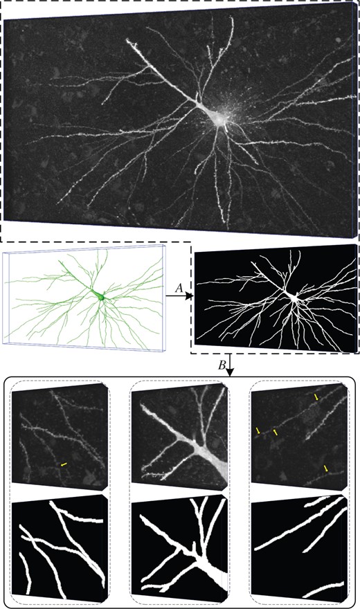
A neuronal image and three cubes cut from it. A: labeling, B: cutting. The cubes are corrupted by random noises; some weak nerve fibers in the cubes are disconnected, as marked by the yellow arrows. The 3D label matrices are shown below the cubes
Selection. In BigNeuron, some neuronal reconstructions do not provide full information (such as nerve fiber radius) of the neurons. For such neuronal images, we cannot correctly label the fibers for segmentation. Therefore, we exclude these neuronal images in designing NeuCuDa. From the remaining 89 neuronal images, we randomly choose 61 images to generate the neuronal cubes for the training of 3D deep networks, and 28 images to generate the testing cubes. The 28 testing images will also be used to evaluate the performance of reconstruction method proposed in Section 2.1.
Labeling. For each of the chosen 89 (61 + 28) neuronal images, we generate a 3D 0-1 label matrix according to its standard digital reconstruction. Every voxel in the images is assigned to 0 (background) or 1 (nerve fiber). An example neuronal image with its 3D label matrix is shown in Figure 7.
Cutting. Neuronal cubes with size of are randomly cut from the 3D image. Meanwhile, their label cubes are cut from the 3D label matrix. Figure 7 shows three example neuronal cubes.
NeuCuDa contains 19251 and 7132 neuronal cubes for the training and testing of 3D WaveUNet, respectively.
3 Results
We first train and evaluate the seven 3D deep networks on NeuCuDa. Then, using the well-trained networks, we segment and reconstruct the neurons in the 28 test neuronal images with the proposed method in Section 2.1.
3.1 3D neuronal cube segmentation
On the 19251 training cubes, we train the 3D U-Nets and 3D WaveUNets for 30 epochs, using stochastic gradient descent (SGD). The training is driven by cross-entropy loss with weights 1, 5 for ‘background’ and ‘nerve fiber’ voxels, to address the imbalances in the cubes. We initially take a learning rate of 0.1 and reduce it following a polynomial decay for each iteration. The batch size, momentum and weight decay are set as 32, 0.9 and 0.0001, respectively. The segmentation performances on the 7132 test cubes are shown in Table 1. We train 3D WaveUNets when various wavelets are used, and for each network architecture, the results of three wavelets are shown in Table 1. In the table, ‘haar’ stands for the Haar wavelet, while ‘dbp’ and ‘ch’ stand for Daubechies with approximation order p and Cohen wavelet with orders , respectively. The filters of these wavelets are shown in Supplementary Material (Supplementary Section S.1).
Segmentation and reconstruction results
| Architecture | Dual | Encoder | Decoder | Wavelet | Segmentation (IoU) | Reconstruction | Parameters | GFLOPs | |||||||||
|---|---|---|---|---|---|---|---|---|---|---|---|---|---|---|---|---|---|
| Structure | Pool | Str-conv | DWT | Unpool | Deconv | Interpolate | IDWT | bga | ner_fib | Mean | ESA | DSA | PDS | ||||
| Baseline (APP2) | – | – | – | – | – | – | – | – | – | – | – | – | 9.3942 | 14.3641 | 0.3573 | – | – |
| 3D U-Net | DS-PU | None | 99.04 | 45.55 | 72.30 | 2.5444 | 7.3450 | 0.2200 | 0.17 | 1.3771 | |||||||
| DS-PDc | None | 99.29 | 53.65 | 76.43 | 2.4046 | 7.1799 | 0.1950 | 0.20 | 1.8010 | ||||||||
| DS-ScIn | None | 99.21 | 52.96 | 76.09 | 2.3614 | 6.9439 | 0.1968 | 0.20 | 1.7990 | ||||||||
| 3D WaveUNet | WADS-DDc | haar | 99.32 | 54.80 | 77.06 | 2.3272 | 6.8841 | 0.1962 | 0.20 | 1.8022 | |||||||
| ch2.2 | 99.32 | 54.58 | 76.95 | 2.2495 | 6.5712 | 0.1956 | |||||||||||
| db3 | 90.27 | 54.76 | 77.02 | 2.3391 | 7.0144 | 0.1931 | |||||||||||
| WADS-DIn | haar | 99.20 | 52.59 | 75.90 | 2.5247 | 7.1783 | 0.2083 | 0.20 | 1.8022 | ||||||||
| ch2.2 | 99.27 | 52.89 | 76.08 | 2.0288 | 6.2569 | 0.1922 | |||||||||||
| db2 | 99.20 | 52.67 | 75.94 | 2.2197 | 6.6692 | 0.1947 | |||||||||||
| WADS-DI | haar | 99.30 | 54.31 | 76.81 | 2.0588 | 6.4043 | 0.1866 | 0.17 | 1.8532 | ||||||||
| ch4.4 | 99.28 | 54.46 | 76.87 | 2.1726 | 6.3609 | 0.1938 | |||||||||||
| db4 | 99.22 | 53.06 | 76.14 | 2.0676 | 6.2566 | 0.1857 | |||||||||||
| WADS-DIDnb | haar | 99.30 | 54.76 | 77.03 | 2.0336 | 6.0730 | 0.1868 | 0.17 | 1.8556 | ||||||||
| ch4.4 | 99.26 | 54.78 | 77.02 | 2.2067 | 6.6038 | 0.1914 | |||||||||||
| db4 | 99.24 | 53.22 | 76.23 | 1.9973 | 6.0173 | 0.1897 | |||||||||||
The bold numbers indicate the best result of various 3D deep networks. a‘bg’ and ‘ner_fib’ are short for ‘background’ and ‘nerve fiber’, respectively.
‘Dn’ stands for ‘Denoising block’.
3D U-Net(PU), applying max-pooling/max-unpooling, performs the worst on neuronal cube segmentation among the seven deep networks. This result suggests that the pair of sampling operations is not suitable for neuron segmentation, which matches our analysis. Comparing the segmentation results of 3D U-Net(PDc) and 3D WaveUNet(DDc), one can find that DWT performs better than max-pooling, when deconvolution is taken as up-sampling operation; 3D WaveUNet(DDc) achieves the best segmentation performance (mIoU, 77.06%).
Among the seven networks, the segmentation performances of 3D U-Net(ScIn) and 3D WaveUNet(DIn) are only better than that of 3D U-Net(PU), which indicates that the linear interpolation used in their decoder is not a good up-sampling operation for 3D neuron segmentation.
3D WaveUNet(DI) and 3D WaveUNet(DIDn), which apply 3D DWT and IDWT for neuron data down-sampling and up-sampling, perform also well for neuronal cube segmentation. Comparing their results, we conclude that denoising on high-frequency components could slightly improve the performance of neuronal cube segmentation. The segmentation performance of 3D WaveUNet(DIDn) is close to that of 3D WaveUNet(DDc), although the convolutions in decoder of 3D WaveUNet(DDc) uses more parameters. In summary, the 3D wavelets improve the performance of neuron segmentation in 3D noisy images.
In Table 1, the last column lists the No. of multiply-add operations required by various 3D deep networks, for processing a neuronal cube with size of . 3D U-Net(PU) applies the simple down-sampling and up-sampling operations, i.e. Max-pooling and Max-unpooling, which takes the least No. of multiply-add operations (1.3771 G). 3D U-Net(PDc) and 3D U-Net(ScIn) apply strided-convolution and DeConv for their down-sampling and up-sampling, which require 1.8010 G and 1.7990 G multiply-add operations, respectively. In 3D WaveUNets, the No. of operations required by wavelet transforms are less than 3% of that of 3D U-Net(PDc) and 3D U-Net(ScIn), while the segmentation and reconstruction performances of 3D WaveUNets are superior.
For segmentation of the 28 test neuronal images, Table 2 shows the average processing time of various 3D deep networks, on an Nvidia V100 GPU. In average, our method needs about two seconds to segment a 3D neuronal image.
Average processing times of various 3D deep networks for segmentation of the 28 test neuronal images
| Architecture | 3D U-Net | 3D WaveUNet | |||||
|---|---|---|---|---|---|---|---|
| Dual structure | PU | PDc | ScIn | DDc | DIn | DI | DIDn |
| Times (s) | 1.4810 | 1.4657 | 1.4703 | 1.7276 | 1.7751 | 2.0980 | 2.1678 |
| Architecture | 3D U-Net | 3D WaveUNet | |||||
|---|---|---|---|---|---|---|---|
| Dual structure | PU | PDc | ScIn | DDc | DIn | DI | DIDn |
| Times (s) | 1.4810 | 1.4657 | 1.4703 | 1.7276 | 1.7751 | 2.0980 | 2.1678 |
The bold numbers indicate the best result of various 3D deep networks.
3.2 3D neuron reconstruction
After segmenting the nerve fibers in the partitioned cubes, we assemble 3D neurons in the 28 test neuronal images, and reconstruct them using APP2, as described in Section 2.1. We evaluate the accuracy of automatic reconstructions by comparing them with the manual one, using three metrics (lower is better), i.e. ‘entire structure average (ESA)’, ‘different structure average (DSA)’ and ‘percentage of different structures (PDS)’, proposed in the study by Peng et al. (2010a). Table 1 shows the three mean metric values of the 28 neurons reconstructed using APP2 on the segmentation results of 3D U-Nets and 3D WaveUNets.
The three mean metric values (9.3942, 14.3641 and 0.3573) of APP2 on the 28 original noisy images are taken as baseline. From Table 1, one can find that the reconstruction performance on the segmented images of the seven deep networks is clearly superior to the baseline, which indicates that our method significantly improves the 3D neuron reconstruction. Generally, with the application of 3D DWT and IDWT in the encoder and decoder of the deep networks, the reconstruction performance is getting better and better, and 3D WaveUNet(DIDn) with wavelet ‘db4’ achieves the best reconstruction performance (1.9973, 6.0173 and 0.1897). In summary, our 3D wavelet and deep network-based method efficiently improve the automatic reconstruction performance for 3D neurons in the noisy images.
Comparing the segmentation and reconstruction results shown in Table 1, we find that the deep network with better segmentation performance may not lead to the better neuron reconstruction, mainly due to the label noises in the dataset NeuCuda. According to the manual reconstructions of neurons in BigNeuron, we design an automatic software to label the neuronal cubes of NeuCuDa. However, during the implementation, some label noises are introduced into the dataset. As Figure 7 shows, some background voxels surrounding the nerve fibers are incorrectly labeled as neuronal voxels. These label noises result in the inconsistency between the neuron segmentation and its final reconstruction.
In Supplementary Material (Supplementary Section S.4), to better illustrate the effectiveness of 3D wavelet integrated deep networks on 3D neuron segmentation and reconstruction, we apply various automatic tracing algorithms to reconstruct the test images segmented by the different 3D deep networks integrated with or without 3D wavelets.
Figure 8 visually shows the reconstructions of an example noisy neuronal image. In Figure 8, the original size of the image is (z-y-x), while the previous deep network-based 3D neuron segmentation methods (Li et al., 2017; Li and Shen, 2020; Wang et al., 2019a) cannot process the neuronal images with such a large size. Figure 8a shows the manual reconstruction of the neuron, which perfectly reflect the neuron morphology. Figure 8b and c shows the reconstructions of APP2 with different parameters on the original neuronal image. The following three subfigures show the reconstructions of APP2 on the neurons segmented by the three 3D U-Nets, and the last four subfigures show that of the four 3D WaveUNets. While the segmentation process takes the three 3D U-Nets about 4.2 s, it takes the four 3D WaveUNets about and 6.4 s, respectively.
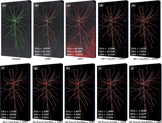
The reconstructions of various methods. (a) The reconstruction manually traced by experts. (b, c) Two reconstructions of APP2 on the original neuronal image, with different parameters. (d–f) The reconstructions of APP2 on the images segmented by the three 3D U-Nets. (g–j) The reconstructions of APP2 on the images segmented by the four 3D WaveUNets. In the reconstructing experiments, we tune two parameters of APP2, i.e. background threshold and length threshold. For the neuron reconstructions shown in (b), we set the two parameters as 10 and 5, respectively, which are the default values in APP2. For the one shown in (c), we set both two parameters as 1. For all the neuron reconstructions traced on the images segmented by 3D deep networks, we set both of the APP2 parameters as 1
On the original noisy image, the automatic tracing algorithm APP2 either stop tracing weak nerve fibers (Fig. 8b) or over-reconstruct strong noises as nerve fibers (Fig. 8c). From Figure 8, one can find that the reconstructions of APP2 on the segmented image are superior to that on the original image, which illustrates the efficiency of our 3D neuron reconstruction method. The 3D U-Nets either classify ‘background’ voxels as ‘nerve fiber’ voxels or do not extract complete nerve fibers. Therefore, their segmented neuronal images contain much background noise (Fig. 8d and e), or the reconstructions are not complete (Fig. 8d and f), as marked by the yellow arrows. The 3D WaveUNets obtain cleaner segmentation and more complete reconstruction, which justifies the effectiveness of 3D wavelets in suppressing noise and keeping nerve fiber structure. Comprehensively, the 3D WaveUNet(DIDn), which utilizes DWT, IDWT and denoising block, achieves the best segmentation and reconstruction results.
We compare our method with three more recent deep networks (Jiang et al., 2021; Li et al., 2017; Li and Shen, 2020). Table 3 lists the results. For ‘3D Residual Net’, we compute the three mean metric values (3.2892, 5.8900 and 0.3367) of APP2 performance on 17 BigNeuron images published in (Li et al., 2017). For ‘3D U-Net Plus’, we reconstruct the neurons in 28 test neuronal images using the well-trained 3D U-Net Plus and reconstruction method, and the reconstruction performance is 33.5020, 40.3151 and 0.5539. On the 28 test neuronal images, the three metrics of ‘Bidirectional Long Short-Term Memory (BLSTM)’ are 6.7582, 13.0149 and 0.3646. While the DSA value (5.8900) of 3D Residual Net is slightly better than that of our method, the network uses significantly more parameters (11.41 M) than our 3D WaveUNets (0.17 M). The performance of 3D U-Net Plus is even inferior to the baseline (shown in Table 1). As the method resizes the neuronal image into before segmentation, it cannot completely segment the neurons in large size neuronal images. BLSTM segment every 2D neuronal slice to denoise the 3D image, which performs badly for disconnected nerve fibers. Comprehensively, among these four methods, our 3D WaveUNets perform best in terms of both metrics and network complexity.
Reconstruction performance of different 3D deep networks
| Network | Reconstruction | Parameters | ||
|---|---|---|---|---|
| ESA | DSA | PDS | ||
| 3D WaveUNet (Ours) | 1.9973 | 6.0173 | 0.1897 | 0.17 |
| 3D residual net (Li et al., 2017) | 3.2892 | 5.8900 | 0.3367 | 11.41 |
| 3D U-Net Plus (Li and Shen, 2020) | 33.5020 | 40.3151 | 0.5539 | 3.60 |
| BLSTM (Jiang et al., 2021) | 6.7582 | 13.0149 | 0.3646 | 0.60 |
The bold numbers indicate the best result of various 3D deep networks.
4 Conclusion
We propose a 3D wavelet and deep learning-based neuron segmentation method, which could improve the reconstruction performance for 3D neurons with large size. We rewrite 3D DWT/IDWT as general network layers, and design the first 3D wavelet integrated encoder–decoder network, 3D WaveUNet, for 3D neuron segmentation. The 3D wavelet transforms could suppress the noise propagation and keep nerve fiber structure during the deep network inference, thus improve the performance of 3D neuron segmentation and reconstruction in noisy neuronal images.
In future, we will study the 3D neuron instance segmentation for images containing multiple neurons and extend the 3D wavelet integrated deep networks to more 3D medical image applications.
Funding
This work was supported by the National Natural Science Foundation of China [62006156, 91959108]; the Science and Technology Project of Guangdong Province [2018A050501014]; and the Science Foundation of Shenzhen [JSGG20180508152022006].
Conflict of Interest: none declared.

