MetaCherchant: analyzing genomic context of antibiotic resistance genes in gut microbiota

Abstract

Motivation

Antibiotic resistance is an important global public health problem. Human gut microbiota is an accumulator of resistance genes potentially providing them to pathogens. It is important to develop tools for identifying the mechanisms of how resistance is transmitted between gut microbial species and pathogens.

Results

We developed MetaCherchant—an algorithm for extracting the genomic environment of antibiotic resistance genes from metagenomic data in the form of a graph. The algorithm was validated on a number of simulated and published datasets, as well as applied to new ‘shotgun’ metagenomes of gut microbiota from patients with Helicobacter pylori who underwent antibiotic therapy. Genomic context was reconstructed for several major resistance genes. Taxonomic annotation of the context suggests that within a single metagenome, the resistance genes can be contained in genomes of multiple species. MetaCherchant allows reconstruction of mobile elements with resistance genes within the genomes of bacteria using metagenomic data. Application of MetaCherchant in differential mode produced specific graph structures suggesting the evidence of possible resistance gene transmission within a mobile element that occurred as a result of the antibiotic therapy. MetaCherchant is a promising tool giving researchers an opportunity to get an insight into dynamics of resistance transmission in vivo basing on metagenomic data.

Availability and implementation

Source code and binaries are freely available for download at https://github.com/ctlab/metacherchant. The code is written in Java and is platform-independent.

Supplementary information

Supplementary data are available at Bioinformatics online.

1 Introduction

The spread of microbes’ resistance to antimicrobial drugs (antibiotic resistance, AR) is a global healthcare problem. Pathogenic microbes with multidrug resistance pose especially high hazard. According to the report of AMR (O’Neill, 2016), the burden of AR-related deaths is predicted to increase to 10 million lives annually by 2050 and the global economic burden—to 100 trillion US dollars. The major factors contributing to the resistance spread are extensive medical and agricultural use of antibiotics (Rolain, 2013).

Human gut microbiota is a reservoir of AR (Sommer et al., 2009).During antibiotic therapy, composition of microbiota and resistome can change drastically (Shashkova et al., 2016; Wright, 2007). Specific genes might increase in abundance because they give their carrier microbe advantage via resistance to the antibiotic. In part, they can be transmitted to other bacterial species through horizontal transfer. In cases when they do not confer resistance to the consumed substance themselves, the dissemination can happen because of the colocalization on the same mobile element with such genes. At the same time, presence of other genes might deplete because of the decreased fraction of their carriers due to the drug action.

Due to active horizontal gene transfer (HGT) within gut microbiota, the increase in resistome, amplified by the number of subjects in world population consuming antibiotics strongly increases the chance for pathogenic microbes to obtain genetic resistance determinants from resistant commensal microbes inhabiting human body. Therefore, identification of resistome dynamics during and after antibiotic intake as well as of the mechanisms of AR transmission within human gut is of utmost actuality.

Metagenomic analysis of gut resistome in populations of the world showed that national specifics of healthcare related to antibiotic usage and socioeconomic factors are reflected in the resistome composition as well as in the extent of its replenishment from the environment (Forslund et al., 2013; Pehrsson et al., 2016). Interestingly, significant levels of AR determinants were also detected in gut metagenomes of isolated populations having no access to antibiotics (Rampelli et al., 2015) thus suggesting the global nature of AR transmission in microbial world.

Isolation and sequencing of individual bacterial genomes allows examining genetic AR determinants at strain level (Dai et al., 2016)—particularly, examining the genomic features surrounding the gene in order to assess the AR transmission history and potential. However, only a small fraction of microbes can be cultivated using state-of-the-art methods, particularly, among gut-dwelling species. On the other hand, each ‘shotgun’ human gut metagenome potentially contains information about all major species present in the community—thus making it possible to predict the data available from sequencing of an isolated strain. It can be performed at the general level of comparing relative abundance of AR genes (Yarygin et al., 2017a,b), as well as at a more detailed level—by exploring the genomic context (environment) of an individual AR gene or operon. Common approaches to this task include metagenomic de novo assembly and subsequent analysis of contigs. The AR genes are identified in the contigs and their genomic context is analyzed to identify the location of the gene within a genome, the composition of the mobile element surrounding the gene and the environment of this element.

Such scenario works well in the case when the gene is present in a single species within a metagenome and occurs exactly once in a genome. However, besides the fact that the genome can contain several AR gene copies, gut microbiota is known to exhibit significant subspecies-level diversity, i.e. multiple subspecies of a single species with diverse genomes (Greenblum et al., 2015). Moreover, within a gut microbiota of a single subject, a gene can be present in several species simultaneously—a phenomenon which is likely to activate under the impact of antibiotics (Crémet et al., 2012; Goren et al., 2010). The mentioned conditions suggest that during ordinary metagenomic assembly the linear contigs are likely to end at the location corresponding to genomic repeats and will provide only an oversimplified consensus image of the real genomic context of AR gene. Such simplified representation does not allow assessing the environment correctly thus impeding the identification of the species—the donor of AR gene and the respective acceptor. A more precise reconstruction of the AR evolution in vivo would improve the efficiency of personalized resistance profiling for a patient and selection of optimal antibiotic therapy scheme. From the perspective of global healthcare, it would facilitate the tracking of significant trends in resistome spread as well as its control.

Here we present MetaCherchant—a method for exploratory analysis of genomic context of genes conferring AR directly from the metagenomic data based on local de Bruijn graph (dBg) assembly. Unlike traditional assembly, MetaCherchant preserves the original unflattened structure of this context thus providing a more accurate description of resistome dynamics in human microbiota. The method was validated using simulated datasets. Its application to gut metagenomes from patients before and after antibiotic therapy revealed evidence of potential horizontal transfer of AR genes between different species.

2 Materials and methods

2.1 Workflow of the algorithm

2.1.1 Partial metagenomic assembly algorithm using a starting point

We developed a novel algorithm that performs classic steps of metagenomic assembly up to the point of construction of dBg using the metagenomic reads. As the result, it builds a subgraph of that graph around a target nucleotide sequence—the AR gene of interest. The algorithm allows analyzing dBg paths that contain the selected sequence thus making it possible to extract more information about the environment of the AR gene in the genome of one or multiple species within the microbiota. The algorithm was implemented basing on previously developed MetaFast software (Ulyantsev et al., 2016) using Java programming language and can be run in parallel mode. The source code is available on GitHub: https://github.com/ctlab/metacherchant.

The first step of the algorithm is decomposing the input metagenomic reads and target sequence into k-mers (nucleotide sequences of length k). The k-mers are stored in a hash table along with their coverage (the total number of times a particular k-mer has appeared in the reads). All the k-mers that are detected with frequency below a fixed threshold are discarded as erroneous.

Due to the specificity of the problem the algorithm aims to solve, it is possible to overcome the k  ≤ 31 restriction and, for larger values of k, only store the hash value instead of the actual k-mer. As the sequence of the target gene is known, it is only necessary to check if some specific k-mer is present in the reads without actually storing all the k-mers. This feature allows increasing memory efficiency of the algorithm and using higher values of k thus providing high-detailed analysis of the graph structure with only a slight loss in performance. Although this solution might produce undesirable hash collisions (because multiple k-mers can be mapped to the same hash value), the frequency of the latter is low compared with sequencing errors. These collisions affect the resulting graph in just a few k-mers that can be easily identified and removed. A trimming function described below automatically processes such collisions.

Then a dBg is constructed using the k-mers obtained from metagenomic data. Vertices in the graph correspond to k-mers, and edges correspond to to (k + 1)-mers. Two vertices in the graph are connected with an edge if the nucleotide sequence on that edge is obtained by joining the vertices’ sequences overlapped by k−1. Genomic environment of a target gene is defined as some subgraph of the dBg containing the gene.

To identify the subgraph, we apply a modification of the standard breadth-first search (BFS) algorithm. In this algorithm, all visited vertices in the dBg are stored in a queue and processed in the order of extraction. Thus, all vertices are added to the subgraph in increasing order of distance from the target gene. Therefore, the target environment subgraph is a set of k-mers closest to the target gene, and the sequences that are close to the target gene are likely to be close to the target gene in the metagenome itself. Two stopping conditions are possible: either the maximum amount of vertices in the subgraph is reached or the maximum distance from the target gene is reached (the user can choose which one to use).

For comprehensive visualization, each long non-branching path in a subgraph is displayed as one long sequence (also known as a unitig). This visualization is achieved by the following algorithm: as long as a pair of vertices can be merged, they are merged. Two vertices are merged when they are connected by an edge and have no other ingoing/outgoing edges. No edge in the graph is processed/examined twice, so the complexity is linear to the size of the graph. The resulting graph is saved in one of several formats including GFA (Graphical Fragment Assembly) and Velvet LastGraph. The graphs can be visualized with any program supporting these formats, including Bandage (Wick et al., 2015).

In single-metagenome mode (default), the algorithm processes a single metagenome to yield a single graph. Differential mode allows comparing genomic environments of the same target gene between two different metagenomes by constructing the combined graph from both datasets. When applied to paired datasets, this functionality allows the user to identify the changes in the environment—e.g. differences in the environment of an AR gene in gut metagenome of a patient before and after antibiotic treatment (such changes indicate possible horizontal transfer event). The algorithm allows finding common and different parts of two subgraphs, detecting overlapping subgraphs for different bacteria and postulating hypotheses about AR gene presence and transfer mechanisms.

As input, MetaCherchant accepts metagenomic reads, single or multiple target gene sequence(s) and configuration parameters. The output of MetaCherchant comprises a dBg in GFA format, a k-mer frequency distribution and a FASTA file with unitigs from the constructed subgraph. Documentation and examples are available at https://github.com/ctlab/metacherchant and in Supplementary Note S1. The workflow of the algorithm is presented in Figure 1. The pseudocode of the algorithm is shown below.

Algorithm 1

Single-mode algorithm workflow

1: Read metagenomic data from files specified in—reads parameter

2: All k-mers are stored in hash map: k-mer → its coverage

3: if$k\le 31$ and –force-hashsing option is not set then

4:  Use k-mer’s 2k-bit representation as key for hash map

5: else

6:  Use hash(k-mer) as key for hash map

7: Read all DNA sequences from file in—seq parameter

8: Create a thread pool

9: for all input sequences in input.fasta file do

10:  run OneSequenceCalculator for this sequence using thread pool

Algorithm 2

Multi-mode algorithm workflow

1: loadInput()

2: Create a thread pool

3: for all input sequences in input.fasta file do

4:  run OneSequenceCalculator for this sequence using thread pool

Algorithm 3

OneSequenceCalculator main routine

1: if—both-dirs option is set then

2:  runBFS({forward, backward})

3: else

4:  runBFS({forward})

5:  runBFS({backward})

6: Save found k-mers as env.txt

7: Merge non-branching k-mers into unitigs

8: Output all unitigs longer than—unitig-length parameter to seqs.fasta

9: Build, color (if applicable) and print graph as graph.gfa

Algorithm 4

runBFS routine

Accepts a subset of {forward, backward} as input.

Outputs a genomic envinronment: a set of k-mers reachable from the starting sequence.

1: Initialize data structures:

• queue—a queue storing all k-mers in order of increasing distance from starting k-mers

• dist—map from k-mer to its distance

• lastKmers—set of k-mers that are a” boundary” of the graph

2: Add all k-mers of the starting sequence to queue with dist equal to 0.

• If none are found, report an error.

3: while the queue is not empty do

4:  Dequeue a k-mer, call it x

5:  for all x’s neighbors in input direction that are present in input reads do

6:   If the max-kmers and max-radius constraints are not violated, add it to queue and dist.

7:   Otherwise, add it to lastKmers set.

8: if–trim-paths option is enabled then

9:  Run the same BFS, but with starting k-mers as lastKmers and input directions reversed

10:  Remove all k-mers that are not visited during this BFS run

11: return All k-mers visited and not removed

Fig. 1.

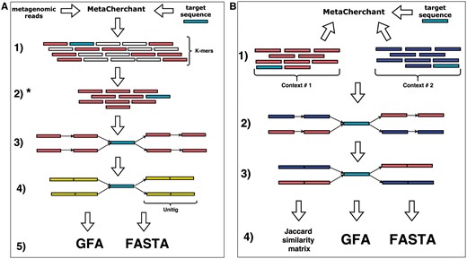
MetaCherchant workflow. (A) Single-metagenome mode (environment-finder function). 1. Read metagenomic data and decompose it into k-mers. 2. Find all k-mers included into the target gene sequence. 3. BFS on the dBg starting from k-mers of target gene. 4. Compress non-branching paths of dBg into unitigs. 5. Save the graph to file in one of supported formats. (B) Differential multi-metagenome mode (environment-finder-multi function). 1. Download k-mers distributions (>2), which were obtained on single-mode. 2. BFS on the dBg starting from k-mers of target gene. 3. Compress non-branching paths of dBg into unitigs. 4. Save the graph to file in one of supported formats. *k-mer frequencies can be used to combine contexts and calculate distances between different contexts

2.1.2 Trimming of genomic environment graph

To correct the effects of sequencing errors and hash collision, a trimming feature was implemented. The feature aims to improve the quality of dBg by removing nodes that are likely to be the result of either an error in the input data or a hash collision when using k > 31. The process of trimming is as follows: when doing BFS, mark all the nodes that could be but were not prolonged because of the termination condition. After that, run a BFS in reverse direction, starting from the marked nodes and only passing through nodes that were visited during the first BFS. This procedure removes all nodes that do not have a path to the ‘border’ of the graph; as a result, all erroneous nodes are removed. However, in case of insufficient coverage, there is a chance that a valid node that was not prolonged is removed.

2.1.3 Choosing k-mer length and coverage threshold

The k-mer length depends on the read length and is user-defined. However, in order to allow the use of environment-finder-multi function, it is required to construct graphs with a fixed value of k because the algorithm uses k-mer frequency distributions to construct the differential graph.

Some k-mers have low coverage because they represent sequencing errors: a sequencing error in one read position can create up to k erroneous k-mers. Filtering of erroneous k-mers improves the resulting graph, makes it more accurate and simplifies the subsequent analysis. The k-mer filtering happens before the construction of dBg. Only those k-mers which occur in input data more often than a specified value of coverage parameter (set by coverage parameter of MetaCherchant) are used by the algorithm. This parameter is set to 5 by default, but the user can select a different value.

2.1.4 Analytical comparison of multiple graphs

We compare two graphs using abundance of k-mers in these graphs. Each k-mer has abundance, which is the number of times it appears in the data. For each k-mer and each graph we calculate this abundance and denote this number as $a{b}_{\text{graph}}(k-mer)$⁠. After that we compute ‘distances’ between every two graphs using following ‘measures’.

$$\begin{array}{c}{J}_{\text{sym}}=1-\frac{|A\cap B|}{|A\cup B|}\\ J_{\text{alt}}=1-\frac{|A\cap B|}{\left|A\right|}\end{array}$$

So these measures belong to [0, 1]. Values around 0 mean that graphs are similar but values around 1 mean difference. In our case these are:

$$\begin{array}{c}{J}_{\text{sym}}(A,B)=1-\frac{\sum \min (a{b}_A\kappa ,a{b}_B\kappa )}{\sum \max (a{b}_A\kappa ,a{b}_B\kappa )}\\ J_{\text{alt}}(A,B)=1-\frac{\sum \min (a{b}_A\kappa ,a{b}_B\kappa )}{\sum a{b}_A\kappa }\end{array}$$

where sums run over $\kappa \in k$-mers.

The distance J_sym is better for graphs which are similar in size. Otherwise, the J_alt is better.

For example, in case when we have $J_{\text{alt}}(A,B)\approx 0$ and $J_{\text{alt}}(B,A)\approx 1$⁠, we can see that $A\supset B$ and A is much greater than B.

2.2 Datasets

MetaCherchant was tested on several simulated and real metagenomic datasets listed in Table 2.

Table 1.

Metagenomic datasets used for testing MetaCherchant algorithm

Dataset	No. metagenomes	No. reads per metagenome (mean ± SD), mln	Sequencing platform (read length, bp)
Simulated metagenomic dataset 1	5	4	N/A (150)
Simulated metagenomic dataset 2	10	5.3 ± 3.0	N/A (250)
Glushchenko_2017	10	17 ± 9	Illumina HiSeq (250)
Korpela_2016	80	14 ± 5	Illumina HiSeq (100)
PRJEB6092 (from EBI)	24	58 ± 14	Illumina HiSeq (100)
Rose_2017	14	19 ± 4	Illumina MiSeq (300)
Willmann_2015	12	68 ± 11	Illumina HiSeq (100)

2.2.1 Simulated data

To validate the algorithm, simulated Illumina pair-end reads were randomly generated from selected microbial genomes using ART (Huang et al., 2011). Single-genome (‘genomic’) simulation was performed using Klebsiella pneumoniae HS11286 genome (Liu et al., 2012). Multi-genome (metagenomic) simulation was performed by randomly mixing the reads simulated from that and other four genomes: Enterococcus faecium EFE10021, Escherichia coli K12, Bifidobacterium longum BG7 and Bacteroides vulgatus ATCC_8482 downloaded from NCBI GenBank database. In each of the simulations, targeted coverage for each of the genomes was 20×. For the insertion simulations, the sequence of AR gene (or a mobile element including the gene) was inserted at a random location of a microbial genome. For the simulation of HGT event that occurred between the first and the second time points (corresponding to two metagenomes), the sequence of K.pneumoniae transposon Tn1331 was inserted into the genome of K.pneumoniae as well as of E.coli. The first metagenome was simulated from the transposon-carrying K.pneumoniae and transposon-free E.coli, and the second—from transposon-carrying K.pneumoniae and transposon-carrying E.coli.

To examine the occurrence of false positive detections (i.e. when a gene is present in a genome but is not displayed in the constructed subgraph due to low coverage), we performed experiments with simulated metagenomes generated from multiple gut microbial genomes including AR genes. Ten sets of metagenomic reads were generated from 10 bacterial genomes, and proportion of reads from each genome was randomly obtained with/by means of exponential distribution using BEAR (Better Emulation for Artificial Reads) (Johnson et al., 2014) software (see Supplementary Tables S1 and S2).

2.2.2 Real sequencing data

The algorithm was applied to ‘shotgun’ metagenomes of stool samples collected from the patients with Helicobacter pylori before and after the H.pylori eradication therapy that included antibiotics intake (Glushchenko et al., 2017). The respective time points were denoted ‘time point 1’ (before the therapy), ‘time point 2’ (immediately after the therapy) and ‘time point 3’ (1 month after the end of the therapy). Datasets from four publicly available sources were used for additional testing of the algorithm (Korpela et al., 2016; Rose et al., 2017; Willmann et al., 2015) (http://www.ebi.ac.uk/metagenomics/projects/ERP005558).

2.3 Data analysis and visualization

Taxonomic profiling of metagenomes was performed using MetaPhlAn2 (Truong et al., 2015). AR genes were identified in the metagenomes by mapping the metagenomic reads to MEGARes database (Lakin et al., 2017) using Bowtie2 (Langmead and Salzberg, 2012). Relative abundance of AR genes was calculated using ResistomeAnalyzer (Lakin et al., 2017). The genomic context of AR genes was obtained by running MetaCherchant in the parallel mode in 10 threads. Taxonomic annotation of sequences corresponding to graph nodes was performed using Kraken (Wood and Salzberg, 2014) and BLAST. Graphs were visualized in Bandage (Wick et al., 2015). Statistical data processing and visualization were conducted in RCoreTeam (2014). Workflow of the data analysis described in the study is shown in Supplementary Figure S1.

2.4 Comparison of SPAdes and MetaCherchant

Genomic context of the target gene was reconstructed with MetaCherchant using preprocessed metagenomic reads and contigs assembled in SPAdes (Bankevich et al., 2012) (parameter: meta). Using the environment-finder-multi function of MetaCherchant, SPAdes contigs were fragmented into k-mers and converted into a graph that was then combined with MetaCherchant graph to identify common and unique segments.

The output of MetaCherchant, MetaPhlAn2 and other analysis results as well as scripts are available at http://download.ripcm.com/Olekhnovich_et_al_2017_MetaCherchant_files/.

3 Results

3.1 Validation of the algorithm on simulated data

In order to check that the algorithm produces correct graph topology around the starting AR gene, we conducted a series of tests on simulated data of increasing complexity (see Supplementary Fig. S2). During the first simulation, we reconstructed the genomic context of a CTX-M (extended-spectrum beta-lactamase) gene naturally included in the genome of K.pneumoniae using simulated reads of this single genome. As expected, the produced graph was linear and the nodes flanking the target gene were annotated correctly. Secondly, in order to assess how the algorithm processes multiple occurrences of a gene in multiple species, the algorithm was applied to reads simulated from two genomes (K.pneumoniae and E.coli) with CTX-M gene sequence introduced into each of them. The obtained graph had a branching structure (Supplementary Fig. S2A); taxonomic annotation of nodes indicates two unique ways of crossing the graph to assemble the fragments of the genomes containing the target gene. The results show that the algorithm correctly reconstructs the gene environment topology in the case when the gene is located in chromosomes of different species.

In the third simulation, we ran the algorithm in differential mode to visualize a simulated HGT of a mobile element containing AR gene from one bacterial species (K.pneumoniae) to another (E.coli) within gut microbiota (see ‘Materials and methods’ Section). The graph visualize the dynamics of genomic environment by combining the subgraphs from two time points—before and after the HGT event—and highlighting the differences between them (Supplementary Fig. 2B). Black color shows the sequences present in each of the metagenomes (all belonging to K.pneumoniae), while the blue color—the sequences that were only present in the second metagenome (all belonging to E.coli), green—K.pneumoniae transposon Tn1331. Thus, our algorithm allows visualizing the transmission of a mobile genomic element between the species. During further simulations, the algorithm correctly reproduced gene environment for CTX-M gene for metagenomes generated from up to five bacterial genomes. The graph complexity increased with the number of genomes, and the values of k and minimum k-mer coverage were adjusted to achieve the most clear result (Supplementary Fig. S2C).

Although the algorithm allows correct detection of genomic context for sufficiently covered AR genes, real metagenomes contain bacterial taxa with widely varying relative abundance. As mentioned, MetaCherchant filters potentially erroneous k-mers basing on the coverage, and in cases of low-abundant microbes or exceeding coverage threshold, certain information about the context of a resistance gene might get lost. To calculate the relation between the coverage depth and abundance of microbes detected in the context, we performed experiments with different simulated coverage on artificial metagenomes containing various proportions of defined microbial species (see Supplementary Fig. S3). As a result, coverage threshold value for a metagenome was estimated to be 1.0 × 10⁹–1.5 × 10⁹ bp to provide optimal detection of AR gene environment. These observations can be used by researchers as guidelines at the phase of metagenomic experiment design to calculate the minimum required coverage of metagenomes. Recommendations for the input metagenomes properties are provided in Supplementary Note S2.

3.2 Analytical comparison of multiple graphs

MetaCherchant constructs metagenomic context graphs that can be visualized in Bandage to gain insights about AR gene environment. However, this method does not produce comprehensive results for multiple graphs. Accordingly, we implemented a function for calculating the Jaccard distance between k-mer distributions during merging contexts (environment-finder-multi tool) that allows comparing AR gene contexts across multiple samples and display such cases as a table. An example of applying this function to simulated data is shown in Supplementary Figure S4.

3.3 Real gut metagenomes: analysis of taxonomic composition and resistome

Real datasets from (Glushchenko et al., 2017) were used to test the algorithm. Before analyzing the genomic environment of AR genes, we assessed the complexity of the gut metagenomes from the patients. As the result of taxonomic analysis, we detected 71 ± 18 species per metagenome in the analyzed gut metagenomes, signifying that the complexity of community structures is similar to the one observed in human gut microbiota studies performed using similar approaches (Tyakht et al., 2013). Within each metagenome, 53 ± 31 AR gene groups were detected. The abundance profiles of AR genes are shown in Figure 2. Presence of multiple AR genes with sufficient coverage suggests that the data is suitable for testing the algorithm.

Fig. 2.

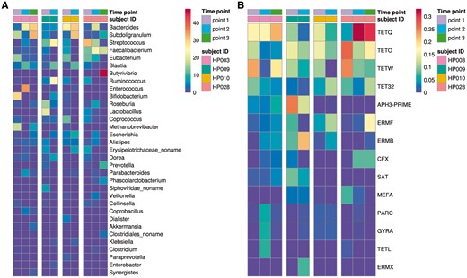
Relative abundance of the major bacterial species and AR gene groups in gut metagenomes (time points and subject IDs are shown in the right-side legend bars as different colors). (A) Relative abundance of major different bacteria species (percent). (B) Relative abundance of major different group AR-genes (mass weight) (Color version of this figure is available at Bioinformatics online.)

3.4 Real gut metagenomes: analysis of AR genes context

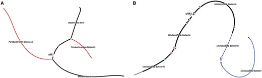
MetaCherchant was applied to explore the context of the major AR genes detected in the metagenomic datasets. For each metagenome, the graph was constructed for the major detected AR gene groups mentioned earlier—specifically, for the most abundant gene of each group (14 ± 8 genes per metagenome, totally 43 genes). The analysis was performed over a range of control parameters (k = 71, minimum allowedk-mer coverage—10×). According to the results of graph reconstruction, some of the AR genes (or highly homologous genes) were detected in a genomic environment of a single bacterial species. An example is adeC gene (multidrug resistance efflux pump) surrounded by sequences classified as E.faecium (Fig. 3A). We identified a structure homologous to transposon of Streptococcus spp. within the genome of S.parasanguinis that contained mel and msrD genes (macrolide resistance efflux pumps) (Fig. 3B). Some of the other genes were surrounded by environments from multiple species: cfxA3 gene (Class A beta-lactamase) together with short additional sequences was surrounded by two related but distinct species—Bacteroides dorei and Parabacteroides distasonis (see Fig. 4, red and black parts of graph). Genomic reconstructions of six other genes (including msrC, cblA and others) showing linear or branching topology of the environment are displayed in Supplementary Figure S5.

Fig. 3.

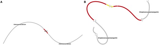
Genomic environment of AR genes reconstructed directly from real gut metagenomes. (A) adeC gene (subject HP_003, time point 2) in genome context E.faecium. Target AR gene is shown in red. (B) A structure homologous to transposon of Streptococcus spp. within the genome of S.parasanguinis that contained mel and msrD genes (macrolide resistance efflux pumps). Target AR genes are shown in yellow; Streptococcus spp. transposon-like structure—in red (Color version of this figure is available at Bioinformatics online.)

Fig. 4.

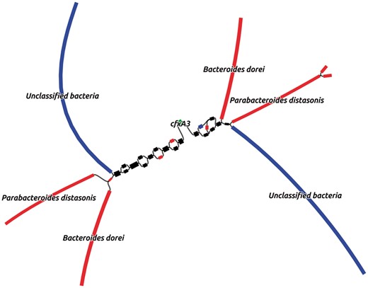
Combined graph of AR gene context produced from two metagenomes of the same subject by running MetaCherchant in differential mode (patient HP_003, cfxA3 gene, time points 2 and 3). Red color denotes the part of the graph present only at the time point 2, blue color—only at the point 3, black—at both points; green color denotes the graph nodes corresponding to the target AR gene (Color version of this figure is available at Bioinformatics online.)

If an AR gene is a part of a large mobile element (>70 Kbp), other mobile elements present in the microbiota are likely to contain sequences with high homology to that element. In such cases, the topology of the obtained graph becomes complex (in part due to presence of multiple adjacent resistance genes) and might include chimeric sequences. Future implementations of the algorithm will allow resolving the distribution of such genes among individual microbial species. Currently, MetaCherchant already allows assessing the mobile genetic elements associated with AR from metagenomic data in an ‘unflattened’ way (without simplifying the graph into contigs). Particularly, it is possible to discover potential associations of an AR gene with a specific taxon or mobile element from the graph. More detailed results are presented in additional materials. An example—graph showing links of ermT and OXA genes to B.dorei genome—is shown in Supplementary Figure S6A.

Due to highly variable abundance of microbial species within microbiota, there are many low-abundant species for which the genomes are incompletely covered by the metagenomic reads. In such cases, when the genomic environment includes uncovered regions, only fragments of the graph can be reconstructed. However, sometimes it is possible to assemble a large part of it, and, when the total length of the fragments is sufficient, to identify the taxonomic annotation of the gene—provided that it is localized on the chromosome; an example of such case is shown for cfxA3 gene in Supplementary Figure S7.

As mentioned above, detection of a microbial genome in the context depends on the coverage and the choice of the coverage threshold. The problem of losing a part of the graph with the increase of coverage threshold is demonstrated in Supplementary Note S3 and Supplementary Figure S8. In order to address this problem, a ‘graph trimming’ function was implemented that allows reducing the noise level while preserving a higher fraction of ‘correct’ k-mers (see Materials and methods).

3.5 Differential mode of MetaCherchant allows identification of possible events of AR gene transmission

Besides the above-described single-metagenome mode, it is possible to run MetaCherchant in differential mode allowing to overlay genomic environments of the same AR gene from several metagenomes. We applied differential mode to paired gut metagenomes obtained from the same subjects before and after antibiotic treatment to identify potential evidence of AR gene transmission—for three subjects in total (HP_003, HP_009 and HP_028, 14 ± 8 genes per metagenome). For some of the genes, it was possible to combine the environments across multiple time points.

An example of such case is displayed in Figure 4: the analysis of the gut metagenomes collected at two time points from a patient potentially shows a transition of cfxA3 gene resistance from one genomic environment to another (red to blue, as shown in the figure)—i.e. appearing to be a HGT event. Taking into account the fact that the two analyzed time points correspond to the samples collected immediately after the H.pylori eradication course and 1 month afterwards, we speculate that the shown graph reflects the specifics of ‘relaxation’ of the gut resistome following the end of antibiotic impact on gut microbiota.

For a single time point, the lack of certain microbial species in AR gene environment can reflect two different effects—when species is absent/low-abundant in microbiota or this gene is not present in the genome of that species. To bring distinction in the case shown in Figure 4, we analyzed read coverage of the context (see Supplementary Fig. S9 and Supplementary Table S5). Although the fragments annotated as ‘Unclassified bacteria’ were included by MetaCherchant only for the time point 3, significant coverage of these sequences by metagenomic reads showed that this microbe is present at all three time points 1–3. Similarly, the species B.dorei and P.distasonis were also present at all time points—however, only at time point 2 they are sufficiently abundant to identify them in the context of this gene (13.80 and 5.95% of total relative abundance, respectively, according to MetaPhlAn2 results). One of the possibilities is that the transposon structure (based on the BLAST results) shown in the graph was present in all these microbes at three time points and the algorithm showed its presence only as the coverage became sufficiently high. To summarize, while the described case of cfxA3 gene does not necessarily reflect a potential HGT event, our method allows generation of hypotheses for further testing using alternative experimental techniques like PCR.

3.6 Comparison with the results of de novo assembly

To assess the efficiency of our tool compared with a related approach—a de novo assembly coupled with a visualization program—we assembled 2 metagenomes from the patient HP_003 using SPAdes and visualized the results in Bandage. We identified the parts of the graph corresponding to cfxA3 gene and compared them to the respective results of MetaCherchant (Fig. 5).

Fig. 5.

Merging of graph environments obtained using SPAdes and MetaCherchant allows comparing the two methods. The environment of cfxA3 gene in metagenomes of subject HP_003 was analyzed. Black color denotes the fragments common for SPAdes and MetaCherchant graphs, red—only the fragments present in MetaCherchant graph, blue—only the fragments present in SPAdes graph. (A) Time point 2. (B) Time-point 3 (Color version of this figure is available at Bioinformatics online.)

The output of SPAdes (Supplementary Fig. S10) corresponded that in the metagenome of subject HP_003 at time point 2 we observe branching in the region of the target gene. However, it is difficult to suggest its possible localization in a mobile element in different bacterial genomes. In the metagenome of the same subject at time point 3, we observe an ambiguous result. The target gene cfxA3 is associated with the unclassified Bacteroides spp.

During formation of contigs, SPAdes algorithm looks for a path in the assembly graph that maximizes the length of the assembly. Here the algorithm selected the only path and the AR gene was placed only into the contig from B.dorei, while no contig(s) of P.distasonis that contained cfxA3 gene were found in the assembly.

The union of the results from MetaCherchant and SPAdes using environment-finder-multi function of MetaCherchant confirmed our hypothesis that SPAdes assembler did not recover the information about genomic environment completely: association of target gene with the genome P.istasonis was lost in this ‘flattened’ representation.

Another disadvantage of assembly using SPAdes is that it is a computationally expensive process. On the other hand, reconstruction of a subgraph around the target gene requires substantially lower computing resources.

3.7 Real gut metagenomes: comparison of multiple datasets

MetaCherchant allows the user to explore the AR gene contexts within multiple sets of metagenomic data. This is useful in the exploration/summary analysis, because it is quite difficult to assess the topology of each single graph visually. In this section, we describe the techniques that allowed us to discover interesting cases and further visualize them.

MetaCherchant was tested on various metagenomic datasets (see Table 2; running options coverage = 5 and k = 41). The summary information on the assemblies is presented in Table 2. The results of an analysis of the distributions of taxa and resistome are presented in Supplementary materials (Supplementary Figs S11 and S12; Supplementary Tables S3 and S4).

Table 2.

Statistics of MetaCherchant assemblies using different datasets (k = 41, coverage = 5)

Dataset	No. unitigs number (mean ± SD)	unitigs length (mean ± SD), kbp, mln	assembly length (mean ± SD), kbp
Glushchenko_2017	1252 ± 1061	0.22 ± 0.34	153 ± 110
Korpela_2017	531 ± 904	0.23 ± 0.10	124 ± 116
PRJEB6092	1747 ± 1106	0.10 ± 0.16	178 ± 97
Rose_2017	253 ± 378	0.31 ± 1.50	79 ± 88
Willmann_2015	681 ± 676	0.18 ± 0.45	124 ± 111

We obtained a set of graphs for the presented AR-genes for each dataset during processing by MetaChechant. With a relatively low read length (100 bp), it is not always possible to assemble an adequate topology of the graph, due to the fact that it is necessary to select low k values. The data from Korpela_2016 dataset had low coverage and it was not always possible to assemble unfragmented context in this case. The most clear results were obtained using Rose_2017 and Glushchenko_2017 datasets—in particular, due to long reads (and subsequent higher k) and sufficient coverage. It is recommended to use data with read length of 250–300 bp and coverage > 2.0 × 10⁹–2.5 × 10⁹ bp for obtaining optimal results. Graphs constructed from the listed datasets are presented in the additional materials at http://download.ripcm.com/Olekhnovich_et_al_2017_MetaCherchant_files/.

3.7.1 Comparison of multiple metagenomes using k-mer frequency distribution

MetaCherchant function environment-finder-multi allows comparing gene environments via dissimilarity of their k-mer frequency spectra (see ‘Materials and methods’ Section), a typical approach for pairwise comparison of metagenomic sequences (reference-free methods) (Benoit, 2016; Dubinkina, 2016). It provides a convenient way for explore the dynamics of the gene context across multiple (>2) samples. As an example of this analysis, distances between multiple metagenomic datasets were computed for two genes—CFX and APH3-Prime (as annotated by MEGAres; see Fig. 6).

Fig. 6.

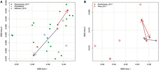
Dissimilarity of k-mer frequency spectra between multiple metagenomic datasets calculated for two genes—CFX (A) and APH3-Prime (B) (Jaccard metric, non-metric MDS). (A) CFX gene. Red arrow shows dynamics for subject HP_003 (transition from time points 2 and 3), blue arrow—similar transition for subject HP_028. (B) APH3-Prime gene. Red and blue arrows show transitions for subject HP_003 (time points 1–3) and subject HP_009 (time points 1–2) (Color version of this figure is available at Bioinformatics online.)

Data shown in Figure 6A suggest that while CFX gene had similar environments in microbiota of subjects HP_003 and HP_028 at time point 2, they became distinct at time point 3, as reflected by the k-mer spectra of the respective graphs. This change is indicated by red (HP_003) and blue (HP_028) arrows. Comparison of k-mer frequency distributions allows performing a comparison even if the topology of respective differential graphs is not obvious (as shown in Supplementary Fig. S13A1 and A2). For example, Supplementary Figure S13A1 and C shows graphs based on the same data (subject HP_003, time points 2 and 3) and the same parameter coverage = 5, but with different values of k. Supplementary Figure S13A1 constructed with k = 41 shows that there is no clear orientation of the unitigs (visual confirmation of potential presence of a gene in several bacterial species). Another clear graph is shown in Supplementary Figure S13C (constructed with k = 83). Rose_2017 dataset containing gut metagenomes of premature infants did not contain the genes of the CFX group, probably due to the absence of Bacteroides genus typically carrying these genes.

We were able to assemble genomic context for APH3-Prime gene for 3 time points for the patient HP_003 (Fig. 6B). The results show a strong context change at the second time point (immediately after taking antibiotics). However, the context becomes again similar to the state before therapy at the third time point. For subject HP_009, we observe a change towards the first time point of subject HP_003. Differential graphs for several time points are shown in Supplementary Figure S13B1–B4. Noteworthy, the samples from Rose_2017 dataset reflect the context for this gene as Staphylococcus aureus, whereas the respective context for Glushchenko_2017 dataset includes E.faecium and other taxa.

Coverage of metagenomes from Korpela_2016 dataset was not sufficient to get adequate reconstruction of the context of CFX and APH3-Prime genes. In most cases, fragmented graphs were obtained for this data set; when comparing by k-mer frequencies, they formed ‘outliers’ distinct from the general cluster.

3.8 Performance

Analysis of metagenomic data was performed on a computational cluster at FRCC PCM on a single 24-core node with 64 Gb RAM; operating system Centos 6.0, Sun Grid Engine scheduler. MetaCherchant was allocated 10 cores.

According to the described experiments, the total time for reconstructing a genomic environment of a single AR gene in a single metagenome (10 threads) was about 11–20 min including data download time (3–5 min), graph reconstruction (<1 min) and taxonomic annotation with Kraken (3–10 min). The relation between the value of k and RAM usage is shown in Supplementary Figure S14.

4 Discussion and conclusions

Gut resistome of healthy humans is distributed among commensal bacteria and does not pose a threat by itself. However, in case of infection with antibiotic-sensitive pathogenic microbes, the AR genes could be transferred from normal microbiota, even from members of a distantly related genus, to the infectious agent. This phenomenon was observed in patients after antibiotic therapy (Crémet et al., 2012; Karami et al., 2007) and demonstrated experimentally on animals and healthy donors (Lester et al., 2004, 2006). Cases of disseminated infections with organisms that acquired resistance genes from the gut microbiota were reported (Crémet et al., 2012; Goren et al., 2010). Thereby, gut microbiota represents an important reservoir of AR genes open to infectious agents of socially significant diseases.

At the moment, two major families of methods for processing metagenomic data are those based on assembly and mapping to reference sequences. Algorithms that include mapping such as MetaPhlAn2 (Truong et al., 2015), MEGAN (Huson et al., 2007), MIDAS (Mielczarek et al., 2013) allowing assessment of relative abundance of microorganisms in environmental samples. By mapping metagenomic reads using algorithms like Bowtie2 (Langmead and Salzberg, 2012), BLAST, DIAMOND (Buchfink et al., 2014), bwa (Li and Durbin, 2009) to reference databases of AR genes [CARD (Jia et al., 2017), MEGARes (Lakin et al., 2017) and other], it is possible to obtain the abundance of the AR genes in the metagenomes. With all the inherent advantages of these approaches, such methods do not allow solving the problems of exploring the localization of genes in the microbial genomes in a reference-independent manner. PanPhlAn (Scholz et al., 2016) and HUMAnN2 (Abubucker et al., 2012) can be used to study bacterial pangenomes. However, these methods have limitations because they work with existing data and some new findings (e.g. HGT events) may not be detected.

Other methods of data analysis implement ‘whole’ assembly of metagenomic reads to contigs based on paradigm of overlap-layout-consensus and dBg. For example, metagenomic assemblers based on dBg are metaSpades (Nurk et al., 2017), Ray Meta (Boisvert et al., 2012), SOAPdenovo2 (Luo et al., 2012), MetaVelvet (Namiki et al., 2012), MEGAhit (Li et al., 2015). However, they possess significant limitations for researchers. For the complete assembly of metagenomes, sufficiently high computational resources are required and the process is very time-consuming. High rate of accumulation of metagenomic information increase this problem. The ‘whole’ assembly is useful when a researcher needs to study the metagenome entirely, carries out de novo assembly of genomes of unknown bacteria and for others similar tasks. This approach is not always relevant, when researcher is performing the task of quickly extracting information from the metagenomes. Thus, there is a need to create algorithms allowing to process large datasets quickly.

An alternative approach that is computationally efficient is to analyze k-mer frequencies from metagenomic data and work with this distribution. In MetaCherchant, k-mers distribution is used to construct a dBg and unify unbranching paths into unitigs. Subsequent taxonomic annotation of unitigs can be performed using a wide range of software. The proposed algorithm allows exploring the connections between AR genes and genomes of taxa present in microbiota using a graph representation. Unlike existing methods, MetaCherchant provides a richer representation of genomic context of AR gene, thus showing the resistance potential of species in gut microbiota in an unbiased way, as well as providing means for examining potential ways of resistance transmission. When compared with an alternative method providing similar results (combination of SPAdes and Bandage), the presented pipeline is simpler and less computationally demanding. It does not require global assembly of the whole graph and its graphic rendering. Moreover, it can also provide more detailed information about the context of the target gene.

Sequencing errors in metagenomic reads hinder reconstruction of gene environment. Filtration of rare k-mers removes noise, but is also associated with deterioration detection of low-abundant microbes. To address this problem, we implemented graph trimming function that simplifies the graph and at the same time filters erroneous k-mers. It provides clearer visualization of metagenomic data and improves accuracy of biological assumptions about potential HGT events and taxonomic annotation of ARGs.

Certain recommendations can be made for a researcher planning to compare metagenomic time series of subjects undergoing antibiotic treatment. At the stage of experiment design of metagenomic survey, in order to provide higher precision of HGT events detection, it is recommended to provide deeper coverage of the initial time point. The reason is that the AR-conferring gene sequences subject to HGT might be insufficiently covered, since they are localized in low-abundant species.

MetaCherchant has certain limitations related to the complexity of graph structures emerging when the AR gene is located within high-covered mobile genetic element. Plasmids and transposons can be present at higher copy number in microbiota than their bacterial hosts—so their coverage can be much higher than one of bacterial chromosomes. When filtering erroneous k-mers, it is required to increase the coverage threshold—but then the display of chromosomal regions becomes deteriorated. Under low coverage threshold, identification of chromosomal sites is possible but the mobile element part of the graph is perplexed by erroneous k-mers. In addition, plasmids and transposons of different taxa can contain highly homologous regions further complicating the graph. These limitations do not allow constructing comprehensive graphs. To overcome the problems of inaccuracy of taxonomic annotations and perception of ‘overcomplicated graphs’, it is logical to include the option of comparing the graphs analytically. We implemented the option of k-mer frequency distribution analysis allowing to compare a multiple datasets independently of the graph complexity. The smaller the reads’ length, the lower value of k can be used for assembly, the greater the proportion of false detections. This method was employed to process five metagenomic datasets obtained on various Illumina platforms (HiSeq, MiSeq) with different read length. The length of the reads at the level of 250–300 bp was sufficient for reconstructing context of target sequences properly. If read length is around 100 bp, the graph created by MetaCherchant is not always visually clear. This approach allowed us to identify differences in the environments of the AP genes, in part, to find interesting cases that can be further accurately visualized.

To summarize, MetaCherchant offers an original representation of genomic environment of AR genes of interest that goes beyond ‘flattened’ images of microbiota diversity provided by traditional methods. The method can be used in metagenomic analytics to compare gene contexts of arbitrary gene of interest. The full-cycle processing and visualization provided by MetaCherchant can be applied not just to gut metagenomes, but also to other environments—it is especially important in the light of discovered transmission of resistance to gut from urban environment (Pehrsson et al., 2016). MetaCherchant will contribute to the design of rational antibiotic therapy schemes for infectious diseases treatment [including the sequence of use of known drugs and introduction of new antimicrobial drugs (Imamovic and Sommer, 2013)]. This will provide both increase of success rate for individual patients and constrain the spread of new multidrug-resistant pathogens.

Acknowledgement

We thank Maria Atamanova (ITMO University) for technical assistance and Igor Buzhinsky, Daniil Chivilikhin and Boris Kovarsky for useful comments.

Funding

Algorithm development was financially supported by the Government of Russian Federation [grant 074-U01]. Algorithm testing and biological application were financially supported by the Russian Scientific Foundation [grant 15-14-00066].

Conflict of Interest: none declared.

Author notes

Evgenii I. Olekhnovich and Artem T. Vasilyev authors wish it to be known that, in their opinion, the first two authors should be regarded as Joint First Authors.