Bias-corrected score decomposition for generalized quantiles

Summary

Decompositions of the score of a forecast represent useful tools for assessing its performance. We consider local score decompositions permitting detailed forecast assessments across a spectrum of conditions of interest. We derive corrections to the bias of the decomposition components in the framework of point forecasts of quantile-type functionals, and illustrate their performance by simulation. Related bias corrections have thus far only been known for squared error criteria.

1. Introduction

The difficulty of making predictions about future data has led to a large literature on the assessment of forecasts. The squared distance between predicted and realized values provides a simple measure of the accuracy, and much existing work relies on quadratic error criteria. Our focus here is on point forecasts of some characteristic of the predictive distribution such as the mean or a quantile. Proper error quantification in this case depends on the concept of a loss type scoring function that is consistent for the given characteristic (Gneiting, 2011). Given such a consistent scoring function, forecaster |$X_1$| would be ranked better than forecaster |$X_2$| if the average score of |$X_1$| is less than that of |$X_2$|⁠. Additional criteria include skill scores (Murphy & Winkler, 1987), calibration and sharpness measures (DeGroot & Fienberg, 1983; Gneiting et al., 2007), as well as decompositions of the average score into three components commonly referred to as reliability, resolution and uncertainty (Murphy & Winkler, 1987; Bröcker, 2009, 2012; Weijs et al., 2010; Christensen, 2015). Comprehensive assessment of forecast schemes requires further information not provided by such summary statistics. Graphical tools such as verification rank histograms are particularly useful for checking the correct calibration of the predictions, but accuracy is also an issue (Gneiting et al., 2007).

We consider score decompositions permitting an assessment of both these aspects. To that end, the data are split into strata according to the values of a variable |$W$|⁠. Usually, only the special case |$W=X$|⁠, where |$X$| is the forecast, is considered. A. Tsyplakov, in the 2014 working paper ‘Theoretical guidelines for a partially informed forecast examiner’ posted at https://mpra.ub.uni-muenchen.de/67333/, points out that the information available to forecasters and assessors may differ, and assessments may be carried out on the basis of any relevant information, encoded here by |$W$|⁠. We specifically consider the case where |$X$| is |$W$|-measurable. Then |$W$| is best thought of as a pair |$W=(X,A)$| where |$A$| represents auxiliary information or indexes domains calling for a separate forecast evaluation, such as season and latitude in weather forecasts (Murphy, 1995). In any case, conditionally on |$W$| the score decomposes into components measuring calibration and entropy locally, in contrast with the common three-term decomposition which involves the intrinsically global resolution and uncertainty terms. Taking up previous findings of a potentially serious bias in estimators of these criteria (Bröcker, 2012; Bentzien & Friederichs, 2014), we derive corrections removing this bias to a first order of approximation. Related results have so far been obtained for mean-value-type functionals and squared error (Ferro & Fricker, 2012). The latter permits algebraic calculations that are not feasible with the scoring functions relevant to quantiles or expectiles. We instead build on a recently established mixture representation of such scoring functions (Ehm et al., 2016) and on the local behaviour of empirical distribution functions. Our bias corrections apply to a broad class of generalized quantiles and the associated consistent scoring functions, making it possible to treat quantiles and expectiles in a unified manner. Likewise, they yield immediate corrections to the bias of global score components such as the resolution.

2. Score decompositions

A characteristic such as a quantile or mean value corresponds to a functional |$F \mapsto T(F)$| on some class |$\mathcal{F}$| of right-continuous distribution functions on the real line, the predictive distributions (Gneiting, 2011). Given |$T$|⁠, a nonnegative scoring function |$S=S(x,y)$| of the point forecast |$x$| of |$T(F)$| and the future observation |$y$| is consistent for |$T$| if for every |$F \in \mathcal{F}$| the expression |$S(x,F) = E_{Y \sim F} S(x,Y)$| is minimized when |$x = T(F)$|⁠; it is strictly consistent if |$x=T(F)$| is the unique minimizer of |$S(x,F)$|⁠. For example, the piecewise linear score |$S(x,y) = |\mathrm{1}_{x<y} - \alpha|\, |x-y|$| is strictly consistent for the lower |$\alpha$|-quantile, |$T(F) = \inf \{t:\, F(t) \ge \alpha\}$|⁠, and the asymmetric quadratic score |$S(x,y) = |\mathrm{1}_{x<y} - \alpha|\, (x-y)^2$| is strictly consistent for the |$\alpha$|-expectile, the solution |$t \equiv T(F)$| of the equation |$(1-\alpha)\int_{-\infty}^t (t-y){\rm d}F(y) = \alpha \int_t^{\infty} (y-{t}){\rm d}F(y)$| (Newey & Powell, 1987). Here |$\mathrm{1}_A$| denotes the indicator function of the event |$A$|⁠, and the respective moments are supposed to be finite for |$F \in \mathcal{F}$|⁠. The case |$\alpha=1/2$| retrieves the median and the mean, which minimize the expected absolute and squared error, respectively.

Throughout the following, |$S$| stands for a fixed scoring function that is consistent for the given functional |$T$| on |$\mathcal{F}$|⁠. The minimum expected score, |$\inf\nolimits_x\, S(x,F) = S\{T(F),F\}$|⁠, is called the entropy of |$F$|⁠, and the overshoot |$d(x,F) = S(x,F) - S\{T(F),F\}$| is called the divergence between |$x$| and |$T(F)$|⁠. In the median and the mean value cases, the entropy reduces to one half times the mean absolute deviation and the variance, respectively, and quite generally it makes sense to think of the entropy as a generalized variance and the divergence as a bias term.

We now consider the point forecast |$x$|⁠, the verifying observation |$y$|⁠, and the third variable |$w$| as a triplet of random variables |$(X,Y,W)$| defined on some probability space |$(\Omega,\mathcal{B},Q)$|⁠. Let |$G$| denote the unconditional, and |$G_w$| the conditional, distribution of |$Y$| given |$W=w$|⁠. All these distributions are supposed to be members of |$\mathcal{F}$|⁠. The random variable |$S\{T(G_W),G_W\}$| quantifies the conditional uncertainty in |$Y$| given |$W$|⁠, to be called the local entropy, |$\small{\text{ENT}}_W$|⁠, and

$$\delta (X,Y\mid W)=E\{S(X,Y)\mid W\}-S\{T(G_W),G_W\}$$

(1)

measures the deviation of the forecast |$X$| from |$T(G_W)$| conditionally on |$W$|⁠, which we call its local miscalibration, |$\small{\text{MCB}}_W $|⁠. If |$X$| is |$W$|-measurable, then |$X$| is fixed whenever |$W$| is fixed, and |$\delta(X,Y\mid W)$| reduces to a divergence in the above sense, |$\delta(X,Y\mid W) = d(X,G_W)$|⁠, hence is nonnegative. In general |$\delta(X,Y\mid W)$| may assume negative values, which does not thwart the technical developments but makes interpretations difficult. Thus for simplicity, we assume that |$X$| is |$W$|-measurable. Rearranging (1) yields a conditional bias variance type decomposition essentially identical to those of Murphy (1995), Bröcker (2009), and Tsyplakov in the paper cited above, namely

$$\begin{gathered} E\{S(X,Y)\mid W\}=\delta (X,Y\mid W)+S\{T(G_W),G_W\} \\ \equiv {\text{MCB}}_W+{\mathrm{E}\mathrm{N}\mathrm{T}}_W\text{.} \end{gathered}$$

(2)

For comparison, the unconditional score decomposition derived in various guises by Brier (1950), Murphy & Winkler (1987), Bröcker (2009) and others, reads

$$\begin{gathered} E\{S(X,Y)\}=E\{\delta (X,Y\mid W)\}-E[d\{T(G),G_W\}]+S\{T(G),G\} \\ \equiv \text{MCB}-\text{RES}+\text{UNC.} \end{gathered}$$

(3)

This results from (2) on writing |$S\{T(G_W),G_W\} = S\{T(G),G_W\} - d\{T(G),G_W\}$| and taking expectations. The global entropy term |$S\{T(G),G\}$| traditionally is called uncertainty, the resolution |$E\, [d\{T(G),G_W\}]$| measures the average variability of |$T(G_W)$|⁠, and the global miscalibration |$\small{\text{MCB}}$| commonly is referred to as the reliability or conditional bias. We deviate from this terminology because we feel that miscalibration is more appropriate than reliability, and because in our setting the term conditional bias is needed for a different purpose.

We assume throughout that |$(x_i,y_i,w_i)\ (i=1,\ldots,n)$| is an independent sample of size |$n$| from |$(X,Y,W)$|⁠. For simplicity, |$W$| is supposed to be discrete, as is effectively the case when the range of |$W$| is partitioned into finitely many bins. The numerical values of the |$w_i$| do not matter in most of the following, and simply are labelled as |$k = 1,\ldots,m$|⁠. Accordingly, |$G_k$| denotes the conditional distribution of |$Y$| given |$W =k$|⁠. We estimate |$G_k$| by the empirical distribution |$\hat G_{n,k}$| of the |$y_i$| such that |$w_i=k$|⁠. Let |$n_k = \# \{i:\, w_i =k\}$| denote their number, and define the local empirical score, entropy, and calibration terms as

$${\overline{S}}_k=n_k^{-1}{\sum }_{w_i=k}S(x_i,y_i),{\widehat{\text{ENT}}}_k=S\{T({\hat{G}}_{n,k}),{\hat{G}}_{n,k}\},{\widehat{\text{MCB}}}_k={\overline{S}}_k-{\widehat{\text{ENT}}}_k\text{.}$$

The empirical analog of (2) then obtains as

$${\overline{S}}_k={\widehat{\text{MCB}}}_k+{\widehat{\text{ENT}}}_k(k=1,\dots ,m),$$

(4)

and the empirical counterparts of the uncertainty and resolution terms are

$$\widehat{\text{UNC}}=S\{T({\hat{G}}_n),{\hat{G}}_n\},\widehat{\text{RES}}=n^{-1}{\sum }_k{n}_k[S\{T({\hat{G}}_n),{\hat{G}}_{n,k}\}-S\{T({\hat{G}}_{n,k}),{\hat{G}}_{n,k}\}],$$

with |$\hat G_n$| the empirical distribution of all |$y_i$|⁠. Writing |$\bar S = n^{-1}\, \sum\nolimits_i S(x_i,y_i)$| for the average score, one obtains the empirical analog of (3),

$$\overline{S}=\widehat{\text{MCB}}-\widehat{\text{RES}}+\widehat{\text{UNC}},$$

(5)

by defining the empirical miscalibration so as to satisfy (5), i.e., as |$\hat {\small{\text{MCB}}} = \bar S + \hat {\small{\text{RES}}} - \hat {\text{UNC}}$|⁠. There is obviously an analogy with the theoretical decompositions: averaging (4) with weights |$n_k/n$| exactly reproduces the global empirical decomposition (5). As a specific feature of (4), all three terms depend only on the forecast-observation pairs |$(x_i,y_i)$| with |$w_i=k$|⁠, and so are strictly local in this sense. By contrast, the empirical resolution and uncertainty terms involve |$T(\hat G_n)$|⁠, and so are global in nature.

3. Correcting the bias of the decomposition components

If the empirical distributions |$\hat G_n$| and |$\hat G_{n,k}$| are close to |$G$| and |$G_k$|⁠, the empirical calibration, resolution, and uncertainty or entropy terms should give useful approximations to their theoretical counterparts. However, there could be a finite sample bias. To study conditional biases given the |$w_i$|⁠, it is convenient to introduce the |$\sigma$|-algebra |$\mathcal{W}$| generated by all indicator variables |$\mathrm{1}_{w_i = k} (i = 1,\ldots,n;\, k = 1,\ldots,m)$|⁠. Frequent use will be made of the following fact.

 

Lemma 1.

Conditionally on |$\mathcal{W}$| the random variables |$y_i$| with |$w_i = k$| are independent and identically distributed with distribution |$G_k$|⁠.

We now show that in order to obtain bias-corrected estimates of the single decomposition components, it suffices to correct for the conditional biases |$\beta_k$| of the local empirical entropies, conditionally on |$\mathcal{W}$|⁠. If |$E^\mathcal{W}$| denotes conditional expectation given |$\mathcal{W}$|⁠, those biases are given by

$${\beta }_k=E^{\mathcal{W}}({\hat{\mathrm{\Delta }}}_k),{\hat{\mathrm{\Delta }}}_k=S\{T({\hat{G}}_{n,k}),{\hat{G}}_{n,k}\}-S\{T(G_k),G_k\}(k=1,\dots ,m)\text{.}$$

(6)

Extensive simplifications result from the local average scores |$\bar S_k$| being unbiased estimates of the respective conditional expectations |$E^\mathcal{W} (\bar S_k) = E\{S(X,Y) \mid W = k\}$|⁠. For by (4), the conditional biases of |$\hat {\small{\text{ENT}}}_k$| and |$\hat {\small{\text{MCB}}}_k$| add to zero, so the bias of the latter term equals |$-\beta_k$|⁠. A similar argument applies to the global miscalibration term

$$\widehat{\text{MCB}}=n^{-1}{\sum }_k{n}_k[{\overline{S}}_k-S\{T({\hat{G}}_{n,k}),{\hat{G}}_{n,k}\}],$$

whose conditional bias is |$-\sum\nolimits_k\, (n_k/n)\, \beta_k$|⁠. Given |$\mathcal{W}$|⁠, the numbers |$n_k$| are known and can be considered as fixed. No such reduction is available for the conditional bias |$\beta = E^\mathcal{W} [S\{T(\hat G_n),\hat G_n\}] - S\{T(G),G\}$| of the empirical uncertainty |$\hat {\small{\text{UNC}}} = S\{T(\hat G_n),\hat G_n\}$|⁠. However, |$\beta$| is again the conditional bias of an empirical entropy, which allows us to determine this bias in complete analogy to that of |$\hat {\small{\text{ENT}}}_k$|⁠. Finally, writing |$\hat {\small{\text{RES}}} = \hat {\small{\text{UNC}}} - (\hat {\small{\text{UNC}}} - \hat {\small{\text{RES}}})$| and recalling |$\hat {\small{\text{UNC}}} - \hat {\small{\text{RES}}} = S\{T(\hat G_{n,k}),\hat G_{n,k}\}$| shows that the conditional bias of the empirical resolution, too, can be expressed in terms of the other biases.

To summarize, suppose that suitable estimates |$\hat \beta_k$| and |$\hat \beta$| of the local and global conditional biases |$\beta_k$| and |$\beta$| are available. Our bias-corrected estimates for the single terms in the decompositions (2), (3) then are constructed as

$$\begin{array}{c}\hfill {\widehat{\text{ENT}}}_k^{\ast }={\widehat{\text{ENT}}}_k-{\hat{\beta }}_k,{\widehat{\text{MCB}}}_k^{\ast }={\widehat{\text{MCB}}}_k+{\hat{\beta }}_k,\end{array}$$

(7)

$$\begin{array}{c}\hfill {\widehat{\text{UNC}}}^{\ast }=\widehat{\text{UNC}}-\hat{\beta },{\widehat{\text{MCB}}}^{\ast }=\widehat{\text{MCB}}+n^{-1}{\sum }_k{n}_k{\hat{\beta }}_k,{\widehat{\text{RES}}}^{\ast }=\widehat{\text{RES}}-\hat{\beta }+n^{-1}{\sum }_k{n}_k{\hat{\beta }}_k\text{.}\end{array}$$

(8)

Clearly, a correction for the conditional bias corrects for the unconditional bias.

 

Remark 1.

The sign of |$\beta_k$| is immediate from (6). Indeed, consistency of |$S$| implies that

$$\begin{array}{c}\hfill E^{\mathcal{W}}[S\{T({\hat{G}}_{n,k}),{\hat{G}}_{n,k}\}]\le E^{\mathcal{W}}\{S(x,{\hat{G}}_{n,k})\}=E^{\mathcal{W}}\{n_k^{-1}{\sum }_{w_i=k}S(x,y_i)\}=S(x,G_k)\end{array}$$

for every |$x$|⁠. Since we may set |$x = T(G_k)$|⁠, it follows that |$E^\mathcal{W} [S\{T(\hat G_{n,k}),\hat G_{n,k}\}] \le S\{T(G_k),G_k\}$|⁠, that is, |$\beta_k \le 0$|⁠. Analogously for the global conditional bias, |$\beta \le 0$|⁠. One notices the similarity with the fact that the empirical variance, with norming |$1/n$|⁠, is biased downwards.

Bias corrections for score decompositions have mainly been studied for mean values. Functionals such as quantiles or expectiles have recently received interest as well (Bentzien & Friederichs, 2014). Their consistent scoring functions share a common form allowing a unified treatment: every such scoring function admits a pointwise valid representation |$S(x,y) = \int S_\theta(x,y)\, {\rm d} M(\theta)$| where |$\{S_\theta, \theta \in R\}$| is a family of elementary scoring functions each of which is consistent for the given functional, and |$M$| is a nonnegative measure on |$R$| (Ehm et al., 2016). One common form of the elementary scoring functions is (Dawid, 2016; Ziegel, 2016)

$$S_{\theta }(x,y)=I_{\theta }(y)1_{\theta <x}+L_{\theta }(y)$$

(9)

where the function |$I_\theta(\,y)$| is nondecreasing in |$\theta$|⁠, and both |$I$| and |$L$| are right-continuous in |$\theta$| for every |$y$|⁠. Specifically, in the case of an |$\alpha$|-quantile the functions are |$I_\theta(\,y) = \mathrm{1}_{y \le \theta}-\alpha, \, L_\theta(\,y) = \alpha\, \mathrm{1}_{y> \theta}$|⁠, while for an |$\alpha$|-expectile |$I_\theta(\,y) = (1-\alpha)(\theta-y)_+ - \alpha (\,y - \theta)_+\, , L_\theta(\,y) = \alpha (\,y - \theta)_+$|⁠, with |$a_+ = a \vee 0,\, a_- = -(a\wedge 0)$| the positive respectively negative part of |$a \in R$|⁠. The |$I_\theta$| form a family of so-called identification functions. The name derives from the fact that they can be used to identify the value |$T(F)$| of the relevant functional at |$F$|⁠. Indeed, |$I_\theta(F) < 0 \Longleftrightarrow \theta < T(F)$|⁠, which follows from the respective definition of |$T(F)$| and the fact that |$\theta \mapsto I_\theta(\,y)$|⁠, hence |$\theta \mapsto I_\theta(F) \equiv \int I_\theta(\,y)\, {\rm dF(\,y)}$|⁠, is nondecreasing and right-continuous.

 

Proposition 1.

(Dawid, 2016). Suppose that |$\{S_\theta\}$| is a family of nonnegative scoring functions of the form (9) with functions |$I_\theta$| such that the mapping |$\theta \mapsto I_\theta(F)$| is well-defined, nondecreasing, and right-continuous for every |$F \in \mathcal{F}$|⁠. Let |$S(x,y) = \int S_\theta(x,y)\, {\rm d}M(\theta)$| where |$M$| is a nonnegative measure on |$R$| such that |$S(x,F) < \infty$| for |$F \in \mathcal{F},\, x \in R$|⁠. Then |$S$| and each |$S_\theta$| is a consistent scoring function for the functional |$T$| on |$\mathcal{F}$| defined as

$$\begin{array}{c}\hfill T(F)=sup\{t:I_t(F)<0\}=inf\{t:I_t(F)\ge 0\}\text{.}\end{array}$$

Henceforth we consider score decompositions and bias corrections within the setting of Proposition 1. Functionals |$T$| of the specified type will be referred to as generalized quantiles. For our main result we need to suppose the following.

 

Assumption 1.

The class |$\mathcal{F}$| contains each conditional distribution |$G_k$|⁠, and for any |$F \in \mathcal{F}$|⁠,

• (i) |$I_\theta^2(F) = \int I_\theta(\,y)^2\,{\rm d}F(y) < \infty$| for every |$\theta$|⁠;

• (ii) |$\theta \mapsto I_\theta(F)$| is continuously differentiable with derivative |$\dot I_\theta(F)> 0 $| at |$\theta = T(F)$|⁠;

• (iii) if |$F_n$| is the empirical distribution function of a sample of size |$n$| from |$F$|⁠, then as |$n \to \infty$| the process |$\theta \mapsto U_{\theta,n} = n^{1/2} \{I_\theta(F_n) - I_\theta(F)\}$|⁠, converges weakly in the Skorohod space |$D(-\infty,\infty)$| to a mean zero Gaussian process |$\{U_\theta\}$| with continuous sample paths (van der Vaart, 1998, Sect. 18.3).

The above assumptions are weak. For |$\alpha$|-quantiles, e.g., |$U_{\theta,n}$| converges weakly to the Brownian bridge process |$B\{F(\theta)\}$| (van der Vaart, 1998, p. 266), which has continuous sample paths since |$\theta \mapsto F(\theta) = I_\theta(F) + \alpha$| is continuous, by (ii).

 

Theorem 1.

Suppose that the mixture measure |$M$| has a continuous density |$m$|⁠. Then under Assumption 1, the random variable |$\hat \Delta_k$| from (6) admits a stochastic approximation by another random variable |$\Delta_k$| such that |$\hat \Delta_k = \Delta_k + o_p(n_k^{-1})$| as |$n_k \to \infty$| and

$$E^{\mathcal{W}}({\mathrm{\Delta }}_k)=-m(t_k)I_{t_k}^2(G_k)/\{2n_k{\dot{I}}_{t_k}(G_k)\},t_k=T(G_k)(k=1,\dots ,m)\text{.}$$

(10)

As in McCullagh (1987, p. 209) we take the expression (10) for |$E^\mathcal{W} (\Delta_k)$| as our approximation to |$\beta_k = E^\mathcal{W} (\hat\Delta_k)$|⁠. Estimates |$\hat \beta_k$| of the local conditional biases to be used with (7), (8) are obtained on substituting the unknown distributions |$G_k$| in (10) by their empirical counterparts |$\hat G_{n,k}$|⁠. The estimate |$\hat \beta$| of the global conditional bias is of the same form, only that |$G_k\, ,\hat G_{n,k}$| have to be replaced by |$G,\, \hat G_n$|⁠, and |$n_k$| by |$n$|⁠. We therefore focus on the local biases.

Most prominent among the mixture scores are those with a constant mixture density |$m$|⁠. For quantiles, |$m\equiv 1$| yields the piecewise linear score, |$S(x,y) = |\mathrm{1}_{x<y} - \alpha|\, |x-y|$|⁠, while for expectiles |$m\equiv 2$| yields the asymmetric quadratic score, |$S(x,y) = |\mathrm{1}_{x<y} - \alpha|\, (x-y)^2$|⁠. These standard choices are presupposed in the following. We first consider the quantile case. Since by condition (ii) every |$F\in \mathcal{F}$| has a continuous density |$f = F'$|⁠, we find that |$I_\theta^2(F) = (1-2\alpha) F(\theta) + \alpha^2,\ \dot I_\theta(F) = f(\theta)$|⁠. When evaluated at |$\theta=q_F$|⁠, |$q_F$| the |$\alpha$|-quantile of |$F$|⁠, this becomes |$I_{q_F}^2(F) = \alpha(1-\alpha),\ \dot I_{q_F}(F) = f(q_F)$|⁠, whence our bias correction assumes the form |$\hat \beta_k = -\alpha(1-\alpha)/\{2 n_k \hat g_k(\hat q_k)\}$| where |$\hat g_k$| and |$\hat q_k$| are estimates of the density |$g_k$| of |$G_k$| and of its |$\alpha$|-quantile, respectively. This is unfortunate in two respects: first, density estimates tend to be unstable; secondly, the crucial term appears in the denominator. Thus unless |$n_k$| is large enough for a kernel estimate to be useful, it appears wise to consider a bias correction only in connection with a parametric model, where |$\hat g_k$| can be estimated by plugging in the parameter estimates. The expectile case presents no such problems. One simply may replace |$G_k$| by |$\hat G_{n,k}$| and |$t_k$| by the empirical |$\alpha$|-expectile |$\hat \eta_k$| of |$\hat G_{n,k}$| in (10). The correction is fully nonparametric as well as local, as it depends only on the empirical distribution of the verifying observations in the respective bin. For |$\alpha=1/2$| the correction simplifies to |$\hat \beta_k = -s_k^2/(2n_k)$|⁠, with |$s_k^2$| the variance of |$\hat G_{n,k}$|⁠. Related results for this case were obtained by Bröcker (2012) and Ferro & Fricker (2012).

4. Simulations

To illustrate the finite sample performance of the bias correction we report a small simulation study. For simplicity, we took |$W=X$|⁠, and adopted a bivariate normal model,

$$X\sim \mathcal{N}(0,{\sigma }_x^2),Y\mid X=x\sim \mathcal{N}(x\gamma ,{\sigma }^2)\equiv G_x$$

(11)

for some |$\gamma > 0$|⁠. Then |$E\, (Y\mid X) = \gamma X$|⁠, so that in the case |$\alpha = 1/2$| of the mean value or the median, forecast |$X$| is perfectly calibrated if and only if |$\gamma=1$|⁠. However, for |$\alpha \neq 1/2$| the forecast is miscalibrated for |$\alpha$|-quantiles and |$\alpha$|-expectiles even if |$\gamma = 1$|⁠. Parameters used in the simulations were |$\sigma_x=2,\, \sigma=1$|⁠, and |$\alpha\in \{0.5,0.9\}$|⁠, |$\gamma\in \{0.8,1\}$|⁠. We generated 5000 random samples each of |$n=200$| data pairs |$(x_i,y_i)$| according to the model (11). The data were grouped into |$m=40$| bins |$B_k$| according to the order statistics of the |$x_i$|⁠, so that every bin contained |$n_k = 5$| data. In this context, |$w_i$| may be thought of as the mean value, denoted |$\bar x_k$|⁠, of the |$x_i$| belonging to |$B_k$|⁠. Accordingly, we approximated the theoretical conditional distribution of |$Y$| given |$X \in B_k$| by |$\mathcal{N}(\bar x_k\gamma,\sigma^2)$|⁠, which is adequate if the |$\bar x_k$|-values are sufficiently dense. The approximation is not applicable to the two boundary bins, which were ignored.

Figure 1 presents simulation results for a normalized miscalibration measure we call deviation, |$\hat {\small{\text{DEV}}}_k = (1 + \hat {\small{\text{MCB}}}_k/ \hat {\small{\text{ENT}}}_k)^{1/2} - 1$|⁠, and its bias-corrected analog |$\hat {\small{\text{DEV}}}_k^*$|⁠, compared against the theoretical quantities |${\small{\text{DEV}}}_k = (1 + {\small{\text{MCB}}}_k/ {\small{\text{ENT}}}_k)^{1/2} - 1$|⁠. Evidently, the local biases were quite large, and the bias reduction moderate to substantial. Similar results hold for the global biases. The bias of the simulated global miscalibration estimates |$\hat {\small{\text{MCB}}}$| normalized by their standard deviation ranged from |$2.4$| to 5 in the important special case |$\alpha = 0.5$|⁠. With bias correction, the corresponding values were between |$0.25$| and |$0.87$|⁠. They were never larger than one half times the uncorrected ones and often substantially smaller.

Fig. 1.

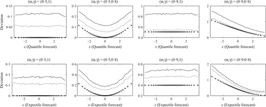
Deviation, i.e., normalized local miscalibration: empirical deviation |$\hat {\small{\text{DEV}}}_k$| averaged across simulations plotted versus likewise averaged forecast bin means |$\bar x_k$| (solid), for four choices of parameters |$\alpha, \gamma$|⁠; same for bias-corrected deviation |$\hat{\small{\text{DEV}}}_k^*$| (dashes) and truth |${\small{\text{DEV}}}_k$| (circles, dots).

5. Discussion

Average scores are widely used to assess forecasts. Conditioning on a third variable yields a decomposition of the average score into local calibration and entropy terms permitting refined assessments. For example, graphical displays of the local decomposition terms can serve as diagnostic tools. The components of the empirical decomposition suffer from a systematic, potentially serious bias. Interestingly, Bentzien & Friederichs (2014) found that these components depend less on the binning when corrected for bias. Our bias correction works binwise, but it can also be used to reduce the bias of the global decomposition terms, where the bias can considerably exceed the dispersion. Throughout the paper it was assumed that the data triplets |$(x_i,y_i,w_i)$| are independent and identically distributed. In fact, the proof of Theorem 1 only requires such an assumption conditionally given |$\mathcal{W}$|⁠, which is weaker.

Acknowledgement

This work was funded by the European Union Seventh Framework Programme. We thank the Klaus Tschira Foundation for infrastructural support at the Heidelberg Institute for Theoretical Studies, and Tilmann Gneiting, the referees, and the editors for their constructive comments.

Appendix

Proof of Theorem 1

Quite generally, |$S_\theta\{T(F),F\} - S_\theta(x,F) = I_\theta(F)\, \{\mathrm{1}_{\theta < T(F)} - \mathrm{1}_{\theta < x}\}$|⁠, by the special form (9) of |$S_\theta$|⁠. Thus by (6) and the mixture representation |$S = \int S_\theta\, {\rm d}M(\theta)$|

$$\begin{array}{c}\hfill {\hat{\mathrm{\Delta }}}_k=\int I_{\theta }({\hat{G}}_{n,k})\{1_{\theta <T({\hat{G}}_{n,k})}-1_{\theta <T(G_k)}\}\mathrm{d}M(\theta )+S\{T(G_k),{\hat{G}}_{n,k}\}-S\{T(G_k),G_k\}\text{.}\end{array}$$

(A1)

For ease of notation we intermediately write |$G_k \equiv F,\, \hat G_{n,k} \equiv \hat F,\, n_k \equiv \nu$|⁠, |$T(G_k) \equiv t, \, T(\hat G_{n,k})\equiv \hat t$|⁠, and |$E^\mathcal{W} \equiv E$|⁠. Since |$I_\theta$| is an identification function, |$\mathrm{1}_{\theta < \hat t} - \mathrm{1}_{\theta < t} = \mathrm{1}_{I_\theta(\hat F) < 0} - \mathrm{1}_{I_\theta(F) < 0} \equiv \chi$|⁠. Clearly |$\chi$| is nonzero only if |$t \wedge \hat t \le \theta < t \vee \hat t$|⁠, or equivalently, if |$I_\theta(\hat F) \wedge I_\theta(F) \le 0 < I_\theta(\hat F) \vee I_\theta(F)$|⁠. Since |$\chi = \pm 1$| according as |$ I_\theta(\hat F) < 0 \le I_\theta(F)$| or |$ I_\theta(F) < 0 \le I_\theta(\hat F) = I_\theta(F) + \nu^{-1/2}\, U_{\theta,\nu}$|⁠, respectively, where |$U_{\theta,\nu} = \nu^{1/2} \{I_\theta(\hat F) - I_\theta(F)\}$|⁠, the integral term in (A1) becomes

$$\int I_{\theta }(\hat{F})(1_{\theta <\hat{t}}-1_{\theta <t})\mathrm{d}M(\theta )=-{\int }_{t\wedge \hat{t}}^{t\vee \hat{t}}|I_{\theta }(F)+{\nu }^{-1/2}{U}_{\theta ,\nu }|\mathrm{d}M(\theta )\text{.}$$

(A2)

Moreover, |$|I_\theta(F) | \le \nu^{-1/2}\, |U_{\theta,\nu}|$| for |$t \wedge \hat t \le \theta < t \vee \hat t$|⁠. Invoking our assumptions we conclude that with arbitrarily high probability |$I_\theta(F) = \dot I_t(F)(\theta-t) + o(\theta-t) = O(\nu^{-1/2})$| for |$\theta$| within this range, which is possible only if |$\hat t - t = O_p(\nu^{-1/2})$|⁠. Note here and for the following that by Lemma 1, |$\hat F$| is the empirical distribution function of a sample of size |$\nu$| from |$F$|⁠. A standard argument as in van der Vaart (1998, § 5.6) then shows that in fact |$\hat t - t \doteq - \nu^{-1/2}\{U_{t,\nu}/\dot I_t(F) + o_p(1)\}$|⁠. Thus by continuity of the density |$m$| of |$M$| we obtain the following approximations, in which |$\doteq$| denotes equality up to terms of order |$o_p(\nu^{-1})$|⁠:

$$\begin{array}{cc}& \hspace{0.17em}{\int }_{t\wedge \hat{t}}^{t\vee \hat{t}}|I_{\theta }(F)+{\nu }^{-1/2}{U}_{\theta ,\nu }|\mathrm{d}M(\theta )\doteq {\int }_{t\wedge \hat{t}}^{t\vee \hat{t}}|{\dot{I}}_t(F)(\theta -t)+{\nu }^{-1/2}{U}_{t,\nu }|m(\theta )\mathrm{d}\theta \hfill \\ & \hspace{0.17em}\doteq {\dot{I}}_t(F)m(t){\int }_{t\wedge \hat{t}}^{t\vee \hat{t}}|\theta -t+{\nu }^{-1/2}{U}_{t,\nu }/{\dot{I}}_t(F)|\mathrm{d}\theta \doteq {\dot{I}}_t(F)m(t){\int }_{t\wedge \hat{t}}^{t\vee \hat{t}}|\theta -\hat{t}|\mathrm{d}\theta \hfill \\ & \hspace{0.17em}={\dot{I}}_t(F)m(t)(t-\hat{t}{)}^2/2\doteq m(t)U_{t,\nu }^2/\{2\nu {\dot{I}}_t(F)\}\text{.}\hfill \end{array}$$

(A3)

In our original notation, the last expression reads |$\, m(t_k) V_{n,k}^2/ \{2n_k \, \dot I_{t_k}(G_k)\} \equiv D_k$| where |$t_k = T(G_k)$|⁠, |$V_{n,k} = n_k^{1/2}\{I_{t_k}(\hat G_{n,k}) - I_{t_k}(G_k)\}$|⁠. Now, let |$\Delta_k = -D_k + S\{T(G_k),\hat G_{n,k}\} - S\{T(G_k),G_k\}$|⁠. Then |$\hat\Delta_k = \Delta_k + o_p(n_k^{-1})$| by (A1) to (A3), and since |$E^\mathcal{W} (\Delta_k) = -E^\mathcal{W} (D_k)$| and |$E^\mathcal{W} (V_{n,k}^2) = I_{t_k}^2(G_k)$|⁠, the theorem follows.