Robust reduced-rank regression

Summary

In high-dimensional multivariate regression problems, enforcing low rank in the coefficient matrix offers effective dimension reduction, which greatly facilitates parameter estimation and model interpretation. However, commonly used reduced-rank methods are sensitive to data corruption, as the low-rank dependence structure between response variables and predictors is easily distorted by outliers. We propose a robust reduced-rank regression approach for joint modelling and outlier detection. The problem is formulated as a regularized multivariate regression with a sparse mean-shift parameterization, which generalizes and unifies some popular robust multivariate methods. An efficient thresholding-based iterative procedure is developed for optimization. We show that the algorithm is guaranteed to converge and that the coordinatewise minimum point produced is statistically accurate under regularity conditions. Our theoretical investigations focus on non-asymptotic robust analysis, demonstrating that joint rank reduction and outlier detection leads to improved prediction accuracy. In particular, we show that redescending $\psi$-functions can essentially attain the minimax optimal error rate, and in some less challenging problems convex regularization guarantees the same low error rate. The performance of the proposed method is examined through simulation studies and real-data examples.

1. Introduction

Given $n$ observations of $m$ response variables and $p$ predictors, denoted by $y_i\in {ℝ}^m$ and $x_i\in {ℝ}^p$ for $i=1,\dots ,n$⁠, we consider the multivariate regression model

$$Y=X{B}^{\ast }+\mathcal{E},$$

where $Y={(y_1,\dots ,y_n)}^{\mathrm{T}}$⁠, $X={(x_1,\dots ,x_n)}^{\mathrm{T}}$⁠, $B^{*}\in {ℝ}^{p\times m}$ is an unknown coefficient matrix, and $\mathcal{E}={(e_1,\dots ,e_n)}^{\mathrm{T}}\in {ℝ}^{n\times m}$ is a random error matrix. Such a high-dimensional multivariate problem, in which both $p$ and $m$ may be comparable to or even exceed the sample size $n$⁠, has drawn increasing attention in both applied and theoretical statistics.

Conventional least-squares linear regression ignores the multivariate nature of the problem and may fail when $p$ is large relative to $n$⁠. Dimension reduction holds the key to characterizing the dependence between responses and predictors in a parsimonious way. Reduced-rank regression (Anderson, 1951; Izenman, 1975) achieves this by restricting the rank of the coefficient matrix, i.e., by solving the problem

$$\begin{array}{c}\hfill \underset{B\in {\mathbb{R}}^{p\times m}}{min}\mathrm{t}\mathrm{r}\{(Y-XB)\mathrm{\Gamma }(Y-XB{)}^{\mathrm{T}}\}\text{subject to\hspace{0.5em}}r(B)\le r,\end{array}$$

(1)

where $tr(\cdot )$ and $r(\cdot )$ denote trace and rank, and $\mathrm{\Gamma }$ is a prespecified positive-definite weighting matrix (Reinsel & Velu, 1998). The ranks are typically much smaller than $m$ and $p$⁠. A global solution to (1) can be obtained explicitly. See Reinsel & Velu (1998) for a comprehensive account of reduced-rank regression under the classical large-$n$ asymptotic regime. Finite-sample theories on rank selection and estimation accuracy of the penalized form of reduced-rank regression were developed by Bunea et al. (2011). The nuclear norm and Schatten $p$-norms can also be used to promote sparsity of the singular values of $B$ or $XB$⁠; see Yuan et al. (2007), Koltchinskii et al. (2011), Rohde & Tsybakov (2011), Agarwal et al. (2012), Foygel et al. (2012) and Chen et al. (2013), among others. Reduced-rank regression is closely connected with principal component analysis, canonical correlation analysis, partial least squares, matrix completion, and many other multivariate methods (Izenman, 2008).

Although reduced-rank regression can substantially reduce the number of free parameters in multivariate problems, it is extremely sensitive to outliers, which are bound to occur; so in real-world data analysis, the low-rank structure could easily be masked or distorted. This is even more serious in high-dimensional or big-data applications. For example, in cancer genetics, multivariate regression is commonly used to explore the associations between genotypical and phenotypical characteristics (Vounou et al., 2010), where employing rank regularization can help to reveal latent regulatory pathways linking the two sets of variables; but pathway recovery should not be distorted by abnormal samples or subjects. As another example, financial time series, even after stationarity transformation, often contain anomalies or have heavier tails than those of a normal distribution, which may jeopardize the recovery of common market behaviours and asset return forecasting; see § 3 in the Supplementary Material.

In this work, we deem explicit outlier detection to be as important as robust low-rank estimation. Indeed, the reduced-rank component may not be of direct interest in some applications, as it often represents common background information shared across the response variables, while capturing unusual changes or jumps is helpful. The robustification of low-rank matrix estimation is nontrivial. A straightforward idea might be to use a robust loss function $\rho$ in place of the squared error loss in (1), leading to

$$\begin{array}{c}\hfill \underset{B}{min}\sum _{i=1}^n\rho \{\Vert {\mathrm{\Gamma }}^{1/2}(y_i-B^{\mathrm{T}}{x}_i){\Vert }_2\}\text{subject to\hspace{0.5em}}r(B)\le r,\end{array}$$

(2)

but such an estimator may be difficult to compute. To the best of our knowledge, even when $\rho$ is Huber’s loss function (Huber, 1981) there is no algorithm for solving (2), let alone when it involves nonconvex losses, which are known to be more effective in dealing with multiple gross outliers with possibly high leverage values. Another motivation is that non-asymptotic theory on the topic is limited. Classical robust analysis, ignoring the low-rank constraint, deals with either deterministic worst-case studies or large-$n$ asymptotics with $p$ and $m$ held fixed, which may not meet modern needs.

We propose a novel robust reduced-rank regression method for concurrent robust modelling and outlier identification. We explicitly introduce a sparse mean-shift outlier component and formulate a shrinkage multivariate regression in place of (2), where $p$ and/or $m$ can be much larger than $n$⁠. The proposed robust reduced-rank regression provides a general framework and includes M-estimation and principal component pursuit (Huber, 1981; Hampel et al., 2005; Zhou et al., 2010; Candès et al., 2011). All the techniques developed in this work apply to high-dimensional sparse regression with a single response. In § 2 we show that low-rank estimation can be ruined by a single rogue point, and propose a robust reduced-rank estimation framework. A universal connection between the proposed robustification and conventional M-estimation is established, regardless of the size of $p$⁠, $m$ or $n$⁠. In § 3 we conduct finite-sample theoretical studies of the proposed robust estimators, with the aim of extending classical robust analysis to multivariate data with possibly large $p$ and/or $m$⁠. A computational algorithm developed in § 4 is easy to implement and leads to a coordinatewise minimum point with theoretical guarantees. Applications to real data are demonstrated in § 5. All the proofs and results of simulation studies, as well as a financial example, are given in the Supplementary Material.

The following notation will be used throughout the paper. We denote by $\mathbb{N}$ the set of natural numbers. We use $a\wedge b$ to denote $\min (a,b)$ and $e$ to denote the Euler constant. Let $\left[n\right]=\{1,\dots ,n\}$⁠. Given any matrix $A$⁠, ${\mathcal{P}}_A$ denotes the orthogonal projection matrix onto the range of $A$⁠, i.e., $A{\left(A^{\mathrm{T}}A\right)}^{\mathrm{-}}{A}^{\mathrm{T}}$⁠, where ${\hspace{0.17em}}^{\mathrm{-}}$ stands for the Moore–Penrose pseudo-inverse. When there is no ambiguity, we also use ${\mathcal{P}}_A$ to denote the column space of $A$⁠. Let $\Vert A{\Vert }_{\mathrm{F}}$ denote the Frobenius norm and $\Vert A{\Vert }_2$ the spectral norm, and let $\Vert A{\Vert }_0=\Vert vec\left(A\right){\Vert }_0=\left|\{(i,j):A(i,j)\ne 0\}\right|$ with $|\cdot |$ denoting the cardinality of the enclosed set. For $A={(a_1\dots a_n)}^{\mathrm{T}}\in {ℝ}^{n\times m}$⁠, $\Vert A{\Vert }_{\mathrm{2,1}}={\displaystyle \sum _{i=1}^n}\Vert a_i{\Vert }_2$ and $\Vert A{\Vert }_{\mathrm{2,0}}={\displaystyle \sum _{i=1}^n}{1}_{\Vert {\alpha }_i\Vert \ne 0}$⁠, which gives the number of nonzero rows of $A$⁠. Given $\mathcal{J}\subset \left[n\right]$⁠, we often denote ${\displaystyle \sum _{i\in \mathcal{J}}}\Vert a_i{\Vert }_2$ by $\Vert A_{\mathcal{J}}{\Vert }_{\mathrm{2,1}}$⁠. Threshold functions are defined as follows.

 

Definition 1

(Threshold function). A threshold function is a real-valued function $\mathrm{\Theta }(t;\lambda )$ defined for $-\infty <t<\infty$ and $0\le \lambda <\infty$ such that (i) $\mathrm{\Theta }(-t;\lambda )=-\mathrm{\Theta }(t;\lambda )$⁠; (ii) $\mathrm{\Theta }(t;\lambda )\le \mathrm{\Theta }(t\prime ;\lambda )$for$t\le t\prime$⁠; (iii) $\underset{t\to \mathrm{\infty }}{lim}\mathrm{\Theta }(t;\lambda )=\mathrm{\infty }$; and (iv) $0\le \mathrm{\Theta }(t;\lambda )\le t$for$0\le t<\infty$⁠.

 

Definition 2

(Multivariate threshold function). Given any $\mathrm{\Theta }$⁠, $\stackrel{\rightharpoonup }{\mathrm{\Theta }}$ is defined for any vector $a\in {\mathbb{R}}^m$ by $\overrightarrow{\mathrm{\Theta }}(a;\lambda )=a\mathrm{\Theta }(\Vert a{\Vert }_2;\lambda )/\Vert a{\Vert }_2$ for $a\ne 0$ and $0$ otherwise. For any matrix $A={(a_1\dots a_n)}^{\text{T}}\in {ℝ}^{n\times m}$⁠, $\overrightarrow{\mathrm{\Theta }}(A;\lambda )=\{\overrightarrow{\mathrm{\Theta }}(a_1;\lambda )\dots \overrightarrow{\mathrm{\Theta }}(a_n;\lambda ){\}}^{\mathrm{T}}$.

2. Robust reduced-rank regression

2.1 Motivation

Although reduced-rank regression is associated with a highly nonconvex problem (1), a global minimizer $\widehat{B}$ can be obtained in explicit form. Given any $r$ such that $1\le r\le \min (m,q)$ with $q=r\left(X\right)$⁠,

$$\begin{array}{c}\hfill \hat{B}(r)=\mathcal{R}(X,Y,\mathrm{\Gamma },r)=(X^{\mathrm{T}}X{)}^{-}{X}^{\mathrm{T}}Y{\mathrm{\Gamma }}^{1/2}{\mathcal{P}}_{V(X,Y,\mathrm{\Gamma },r)}{\mathrm{\Gamma }}^{-1/2},\end{array}$$

(3)

where $V(X,Y,\mathrm{\Gamma },r)$ is formed by the leading $r$ eigenvectors of ${\mathrm{\Gamma }}^{1/2}{Y}^{\mathrm{T}}{\mathcal{P}}_{X}Y{\mathrm{\Gamma }}^{1/2}$⁠; see, e.g., Reinsel & Velu (1998) for a detailed justification. When $\mathrm{\Gamma }=I$⁠, we abbreviate $\mathcal{R}(X,Y,I,r)$ to $\mathcal{R}(X,Y,r)$⁠. The reduced-rank regression estimator is denoted by $\widehat{B}\left(r\right)$ to emphasize its dependence on the regularization parameter.

Outliers are unavoidable in real data. We define the finite-sample breakdown point for an arbitrary estimator $\widehat{B}$ in the spirit of Donoho & Huber (1983): given finite data $(X,Y,\mathrm{\Gamma })$ and an estimator $\widehat{B}(X,Y,\mathrm{\Gamma })$⁠, its breakdown point is

$$\begin{array}{c}\hfill {ϵ}^{\ast }(\hat{B})=\frac{1}{n}min\left\{k\in \mathbb{N}\cup \{0\}:\underset{\tilde{Y}\in {\mathbb{R}}^{n\times m}:\Vert \tilde{Y}-Y{\Vert }_0\le k}{sup}\Vert X\hat{B}(X,\tilde{Y},\mathrm{\Gamma }){\Vert }_{\mathrm{F}}=+\mathrm{\infty }\right\}\text{.}\end{array}$$

In addition to the reduced-rank regression estimator $\widehat{B}\left(r\right)$⁠, we take into account a general low-rank estimator obtained by imposing a singular value penalty

$$\begin{array}{c}\hfill \hat{B}(\lambda )\in \underset{B}{\arg min}\frac{1}{\mathrm{2}}\mathrm{t}\mathrm{r}\{(Y-XB)\mathrm{\Gamma }(Y-XB{)}^{\mathrm{T}}\}+\sum _{s=1}^{p\wedge m}P({\sigma }_s^{B{\mathrm{\Gamma }}^{1/2}};\lambda )\text{.}\end{array}$$

(4)

Here $\lambda$ is a regularization parameter and the ${\sigma }_s^{B{\mathrm{\Gamma }}^{1/2}}$ are the singular values of $B{\mathrm{\Gamma }}^{1/2}$⁠. The penalty $P$ is constructed from an arbitrary thresholding rule $\mathrm{\Theta }(\cdot ;\lambda )$ by

$$P(t;\lambda )-P(0;\lambda )=P_{\mathrm{\Theta }}(t;\lambda )+q(t;\lambda ),P_{\mathrm{\Theta }}(t;\lambda )={\int }_0^{|t|}[sup\{s:\mathrm{\Theta }(s;\lambda )\le u\}-u]\mathrm{d}u,$$

(5)

for some nonnegative $q(\cdot ;\lambda )$ satisfying $q\{\mathrm{\Theta }(s;\lambda );\lambda \}=0$ for all $s\in ℝ$⁠.

 

Theorem 1

Given any finite $(X,Y,\mathrm{\Gamma })$ and $r\ge 1$ with $\mathrm{\Gamma }$ positive definite and $X\ne 0$⁠, let $\widehat{B}\left(r\right)$ be a reduced-rank regression estimator which solves (1). Then its finite-sample breakdown point is exactly $1/n$⁠. Furthermore, for any $\widehat{B}\left(\lambda \right)$ as in (4), ${ϵ}^{*}\left\{\widehat{B}\left(\lambda \right)\right\}=1/n$still holds for any finite value of $\lambda$.

The result indicates that a single outlier can completely ruin low-rank matrix estimation, whether one applies a rank constraint or, say, a Schatten $p$-norm penalty. This limits the use of ordinary rank reduction in big-data applications. Because with the low-rank constraint, directly using a robust loss function as in (2) may result in nontrivial computational and theoretical challenges, we will apply a novel additive robustification, motivated by She & Owen (2011).

2.2 The additive framework

We introduce a multivariate mean-shift regression model to explicitly encompass outliers:

$$Y=X{B}^{\ast }+C^{\ast }+\mathcal{E},$$

(6)

where $B^{*}\in {ℝ}^{p\times m}$ gives the matrix of coefficients, $C^{*}\in {ℝ}^{n\times m}$ describes the outlying effects on $Y$⁠, and $\mathcal{E}\in {ℝ}^{n\times m}$ has independently and identically distributed rows following $N(0,\mathrm{\Sigma })$⁠. Obviously, this leads to an overparameterized model, so we must regularize the unknown matrices appropriately. We assume that $B^{*}$ has low rank and $C^{*}$ is a sparse matrix with only a few nonzero entries because outliers are inconsistent with the majority of the data. Given a positive-definite weighting matrix $\mathrm{\Gamma }$⁠, we propose the robust reduced-rank regression problem

$$\begin{array}{c}\hfill \underset{B,C}{min}\frac{1}{\mathrm{2}}\mathrm{t}\mathrm{r}\{(Y-XB-C)\mathrm{\Gamma }(Y-XB-C{)}^{\mathrm{T}}\}+P(C;\lambda )\text{subject to\hspace{0.5em}}r(B)\le r\text{.}\end{array}$$

(7)

Here $P(\cdot ;\lambda )$ is a sparsity-promoting penalty function with $\lambda$ to adjust the amount of shrinkage, but it can also be a constraint, such as in (12). The following form of $P$ can handle elementwise outliers:

$$\begin{array}{c}\hfill P(C;\lambda )=\sum _{i=1}^n\sum _{k=1}^{m}P(|c_{i,k}|;\lambda )\text{.}\end{array}$$

(8)

It is more common in robust statistics to assume outlying samples, or outlying rows in $(Y,X)$⁠, which corresponds to

$$\begin{array}{c}\hfill P(C;\lambda )=\sum _{i=1}^{n}P(\Vert c_i{\Vert }_2;\lambda ),\end{array}$$

where $c_i^{\mathrm{T}}$ is the $i$th row vector of $C$⁠. Unless otherwise specified, we consider row-wise outliers. But all our algorithms and analyses can handle elementwise outliers after simple modification.

In the literature on reduced-rank regression, it is common to regard the weighting matrix $\mathrm{\Gamma }$ as known (Reinsel & Velu, 1998; Yuan et al., 2007; Izenman, 2008). The choice of $\mathrm{\Gamma }$ is flexible and is usually based on a pilot covariance estimate $\widehat{\mathrm{\Sigma }}$⁠. For example, it can be ${\widehat{\mathrm{\Sigma }}}^{-1}$ when $\widehat{\mathrm{\Sigma }}$ is nonsingular, or a regularized version ${(\widehat{\mathrm{\Sigma }}+\delta I)}^{-1}$ for some $\delta >0$⁠. Although it sounds intriguing to consider jointly estimating the high-dimensional mean and the even higher-dimensional covariance matrix in the presence of outliers, this is beyond the scope of the present paper. When a reliable estimate of $\mathrm{\Sigma }$ is unavailable, a standard practice in finance and econometric forecasting is to reduce $\mathrm{\Gamma }$ to a diagonal matrix or, equivalently, an identity matrix after robustly scaling the response variables. For ease of presentation, we shall take $\mathrm{\Gamma }$ to be the identity matrix, unless otherwise noted, and mainly focus on the following robust reduced-rank regression criterion:

$$\begin{array}{c}\hfill \underset{B,C}{min}\frac{1}{\mathrm{2}}\Vert Y-XB-C{\Vert }_{\mathrm{F}}^2+P(C;\lambda )\text{subject to\hspace{0.5em}}r(B)\le r\text{.}\end{array}$$

(9)

We show that the proposed additive outlier characterization indeed comes with a robustness guarantee and, interestingly, generalizes M-estimation to the multivariate rank-deficient setting. We write $Y={(y_1,\dots ,y_n)}^{\mathrm{T}}$ and $C={(c_1,\dots ,c_n)}^{\mathrm{T}}$⁠.

 

Theorem 2

(i) Suppose that$\mathrm{\Theta }(\cdot ;\lambda )$is an arbitrary thresholding rule satisfying Definition 1, and let$P$be any penalty associated with$\mathrm{\Theta }$through (5). Consider

$$\begin{array}{c}\hfill \underset{B,C}{min}\frac{1}{\mathrm{2}}\Vert Y-XB-C{\Vert }_{\mathrm{F}}^2+\sum _{i=1}^{n}P(\Vert c_i{\Vert }_2;\lambda )\mathit{s}\mathit{u}\mathit{b}\mathit{j}\mathit{e}\mathit{c}\mathit{t}\mathit{t}\mathit{o}r(B)\le r\text{.}\end{array}$$

(10)

For any fixed $B$⁠, a globally optimal solution for $C$ is $C\left(B\right)=\stackrel{\rightharpoonup }{\mathrm{\Theta }}(Y-XB;\lambda )$⁠. By profiling out $C$ with $C\left(B\right)$, (10) can be expressed as an optimization problem with respect to $B$ only, and it is equivalent to the robust M-estimation problem

$$\begin{array}{c}\hfill \underset{B}{min}\sum _{i=1}^n\rho (\Vert y_i-B^{\mathrm{T}}{x}_i{\Vert }_2;\lambda )\mathit{s}\mathit{u}\mathit{b}\mathit{j}\mathit{e}\mathit{c}\mathit{t}\mathit{t}\mathit{o}r(B)\le r,\end{array}$$

(11)

where the robust loss function$\rho$is given by

$$\rho (t;\lambda )={\int }_0^{|t|}\psi (u;\lambda )\mathrm{d}u,\psi (t;\lambda )=t-\mathrm{\Theta }(t;\lambda )\text{.}$$

(ii) Given$\varrho \in \{\mathrm{0,1},\dots ,n\}$, consider

$$\begin{array}{c}\hfill \underset{B,C}{min}\frac{1}{\mathrm{2}}\Vert Y-XB-C{\Vert }_{\mathrm{F}}^2\mathit{s}\mathit{u}\mathit{b}\mathit{j}\mathit{e}\mathit{c}\mathit{t}\mathit{t}\mathit{o}r(B)\le r,\Vert C{\Vert }_{2,0}\le \varrho \text{.}\end{array}$$

(12)

Similarly, (12), after profiling out$C$, can be expressed as an optimization problem with respect to$B$only, and it is equivalent to the rank-constrained trimmed least-squares problem

$$\begin{array}{c}\hfill \underset{B}{min}\frac{1}{\mathrm{2}}\sum _{i=1}^{n-\varrho }{r}_{(i)}\mathit{s}\mathit{u}\mathit{b}\mathit{j}\mathit{e}\mathit{c}\mathit{t}\mathit{t}\mathit{o}r(B)\le r,r_i=\Vert y_i-B^{\mathrm{T}}{x}_i{\Vert }_2,\end{array}$$

where$r_{\left(1\right)},\dots ,r_{\left(n\right)}$are the order statistics of$r_1,\dots ,r_n$satisfying$\left|r_{\left(1\right)}\right|\le \cdots \le \left|r_{\left(n\right)}\right|$⁠.

 

Remark 1

Theorem 2 connects $P$ to $\rho$ through $\mathrm{\Theta }$⁠. As is well known, changing the squared error loss to a robust loss amounts to designing a set of multiplicative weights for $y_i-B^{\mathrm{T}}{x}_i$ (⁠$i=1,\dots ,n$⁠). Our additive robustification achieves the same robustness but leaves the original loss function untouched. The connection is also valid in the case of elementwise outliers, with $P$ and $\rho$ applied in an elementwise manner. In fact, the identity constructed in Lemma 2 of the Supplementary Material,

$$\frac{1}{\mathrm{2}}\{r-\mathrm{\Theta }(r;\lambda ){\}}^2+P_{\mathrm{\Theta }}\{\mathrm{\Theta }(r;\lambda );\lambda \}={\int }_0^{|r|}\psi (t;\lambda )\mathrm{d}t(r\in \mathbb{R}),$$

implies that the equivalence holds much more generally, with $B$ subject to an arbitrary constraint or penalty, regardless of the number of response variables and the number of predictors. This extends the main result of She & Owen (2011) to multiple-response models with $p$ possibly larger than $n$⁠.

 

Remark 2

Theorem 2 holds for all thresholding rules, and commonly used convex and nonconvex penalties are all covered by (5). For example, the convex group ${\ell }_1$ penalty $\lambda {\displaystyle \sum }\Vert c_i{\Vert }_2$ is associated with the soft-thresholding ${\mathrm{\Theta }}_S(s;\lambda )=\text{sgn}\left(s\right){\left(\right|s|-\lambda )}_{+}$⁠. The group ${\ell }_0$ penalty $({\lambda }^2/2){\displaystyle \sum _{i=1}^n}{1}_{\Vert c_i{\Vert }_2\ne 0}$ can be obtained from (5) with the hard-thresholding ${\mathrm{\Theta }}_H(s;\lambda )=s{1}_{\left|s\right|>\lambda }$ and with $q(t;\lambda )=0.5{(\lambda -|t\left|\right)}^2{1}_{0<\left|t\right|<\lambda }$⁠. Our $\mathrm{\Theta }$-$P$ coupling framework also covers ${\ell }_p$ for $0<p<1$⁠, the smoothly clipped absolute deviation penalty (Fan & Li, 2001), the minimax concave penalty (Zhang, 2010a), and the capped ${\ell }_1$ penalty (Zhang, 2010b) as particular instances; see She (2012).

 

Remark 3

The universal link between (10) and (11) provides insight into the choice of regularization. It is easy to verify that the ${\ell }_1$-norm penalty as commonly used in variable selection leads to Huber’s loss, which is prone to masking and swamping and may fail with even moderately leveraged outliers occurring. To handle gross outliers, redescending $\psi$-functions are often advocated, which amounts to using nonconvex penalties in (10). For example, Hampel’s three-part $\psi$ (Hampel et al., 2005) can be shown to yield Fan and Li’s smoothly clipped absolute deviation penalty; the skipped mean $\psi$ corresponds to the exact ${\ell }_0$ penalty; and rank-constrained least trimmed squares can be rephrased as the ${\ell }_0$-constrained form in (12). Our approach not only provides a unified way to robustify low-rank matrix estimation but also facilitates theoretical analysis and computation of reduced-rank M-estimators in high dimensions.

2.3 Connections and extensions

Before we dive into theoretical study, it is worth pointing out some connections and extensions of the proposed framework. First, one can set $\mathrm{\Gamma }$ equal to the inverse covariance matrix of the response variables to perform robust canonical correlation analysis; see Reinsel & Velu (1998). Although we mainly focus on the rank-constrained form, there is no difficulty in extending our discussion to

$$\underset{B,C}{min}\frac{1}{\mathrm{2}}\Vert Y-XB-C{\Vert }_{\mathrm{F}}^2+\sum _{s=1}^{p\wedge m}{P}_B({\sigma }_s^B;{\lambda }_B)+P_C(C;{\lambda }_C),$$

(13)

where the ${\sigma }_s^B$ are the singular values of $B$⁠, and $P_B$ and $P_C$ are sparsity-inducing penalties.

Our robust reduced-rank regression subsumes a special but important case, $Y=B+C+\mathcal{E}$⁠. This problem is perhaps less challenging than its supervised counterpart, but has wide applications in computer vision and machine learning (Wright et al., 2009; Candès et al., 2011).

Finally, our method can be extended to reduced-rank generalized linear models; see, for example, Yee & Hastie (2003) and She (2013) for computational details. In these scenarios, directly robustifying the loss can be messy, but a sparse outlier term can always be introduced without altering the form of the given loss, so that many algorithms designed for fitting ordinary generalized linear models can be seamlessly applied.

3. Non-asymptotic robust analysis

Theorem 2 provides robustness and some helpful intuition for the proposed method, but it might not be enough from a theoretical point of view. For example, can one justify the need for robustification in estimating a matrix of low rank? Is using redescending $\psi$-functions still preferable in rank-deficient settings? Unlike in traditional robust analysis, we cannot assume an infinite sample size and a fixed number of predictors or response variables, because $p$ and/or $m$ can be much larger than $n$ in modern applications. Conducting non-asymptotic robust analysis would be desirable. The finite-sample results in this section contribute to this type of robust analysis.

For simplicity we assume that the model is given by $Y=X{B}^{*}+C^{*}+\mathcal{E}$⁠, where $\mathcal{E}$ has independent and identically distributed $N(0,{\sigma }^2)$ entries, and consider the robust reduced-rank regression problem defined in (9). The noise distribution can be more general. For example, in all of the following theorems except Theorem 5, $\mathcal{E}$ can be sub-Gaussian. Given an estimator $(\widehat{B},\widehat{C})$⁠, we focus on its prediction accuracy measured by $M(\widehat{B}-B^{*},\widehat{C}-C^{*})$⁠, where

$$M(B,C)=\Vert XB+C{\Vert }_{\mathrm{F}}^2\text{.}$$

This predictive learning perspective is always legitimate in evaluating the performance of an estimator, and requires no signal strength or model uniqueness assumptions. The ${\ell }_2$-recovery of $M(\widehat{B}-B^{*},\widehat{C}-C^{*})$ is fundamental, and such a bound, together with additional regularity assumptions, can easily be adapted to obtain estimation error bounds in different norms as well as selection consistency (Ye & Zhang, 2010; Lounici et al., 2011); see Theorem 10 in the Supplementary Material, for instance. Given a penalty function $P$ or, equivalently, a robust loss $\rho$⁠, we will study the performance of the set of global minimizers to show the ultimate power of the associated method; but our techniques of proof apply more generally (see, e.g., Theorem 7).

For any $C={(c_1,\dots ,c_n)}^{\mathrm{T}}$⁠, define

$$\begin{array}{c}\hfill \mathcal{J}(C)=\{i:c_i\ne 0\},J(C)=|\mathcal{J}(C)|=\Vert C{\Vert }_{2,0}\text{.}\end{array}$$

We let $r^{*}=r\left(B^{*}\right)$ denote the rank of the true coefficient matrix, and $J^{*}=J\left(C^{*}\right)$ the number of nonzero rows in $C^{*}$⁠, i.e., the number of outliers. Let $q=r\left(X\right)$⁠.

To handle problems in arbitrary dimensions, we construct some finite-sample oracle inequalities (Donoho & Johnstone, 1994). The first theorem considers a general penalty $P(C;\lambda )={\displaystyle \sum _{i=1}^n}P(\Vert c_i{\Vert }_2;\lambda )$⁠. Here we assume that $P(\cdot ;\lambda )$ takes $\lambda$ as the threshold parameter and satisfies

$$\begin{array}{c}\hfill P(0;\lambda )=0,P(t;\lambda )\ge P_H(t;\lambda ),\end{array}$$

(14)

where $P_H(t;\lambda )=(-t^2/2+\lambda |t\left|\right)1_{\left|t\right|<\lambda }+({\lambda }^2/2)1_{\left|t\right|\ge \lambda }$⁠. The latter inequality is natural in view of (5), because a shrinkage estimator with $\lambda$ as the threshold is always bounded above by the hard-thresholding function ${\mathrm{\Theta }}_H(\cdot ,\lambda )$⁠. From Theorem 2, (14) covers all $\psi$-functions bounded below by the skipped mean ${\psi }_H(s;\lambda )=s{1}_{\left|s\right|\le \lambda }$ for any $s\ge 0$⁠.

 

Theorem 3

Let$\lambda =A\sigma {(m+\log n)}^{1/2}$with$A$a constant, and let$(\widehat{B},\widehat{C})$be a global minimizer of (9). Then, for any sufficiently large$A$⁠, the following oracle inequality holds for any$(B,C)\in {ℝ}^{p\times m}\times {ℝ}^{n\times m}$satisfying $r\left(B\right)\le r$⁠:

$$\begin{array}{c}\hfill E\{M(\hat{B}-B^{\ast },\hat{C}-C^{\ast })\}\lesssim M(B-B^{\ast },C-C^{\ast })+{\sigma }^2(q+m)r+P(C;\lambda )+{\sigma }^2,\end{array}$$

(15)

where $\lesssim$ means that the inequality holds up to a multiplicative constant.

 

Corollary 1

Under the same conditions as in Theorem 3, if$r\ge 1$and$P$is a bounded nonconvex penalty satisfying$P(t;\lambda )\lesssim {\lambda }^2$for any$t\in ℝ$⁠, then

$$\begin{array}{c}\hfill \begin{array}{cc}& E\{M(\hat{B}-B^{\ast },\hat{C}-C^{\ast })\}\hfill \\ & \hspace{0.17em}\lesssim \underset{(B,C):r(B)\le r}{inf}\{M(B-B^{\ast },C-C^{\ast })+{\sigma }^2(q+m)r+{\sigma }^{2}J(C)m+{\sigma }^{2}J(C)\log n\}\text{.}\hfill \end{array}\end{array}$$

(16)

 

Remark 4

Both (15) and (16) involve a bias term $M(B-B^{*}$⁠, $C-C^{*})$⁠. Upon setting $r=r^{*}$⁠, $B=B^{*}$ and $C=C^{*}$ in, say, (16), we obtain a prediction error bound of the order

$$\begin{array}{c}\hfill {\sigma }^2(q+m)r^{\ast }+{\sigma }^2{J}^{\ast }(m+\log n)\text{.}\end{array}$$

(17)

On the other hand, the presence of the bias term ensures applicability of robust reduced-rank regression to weakly sparse $C^{*}$⁠, and similarly $r$ may also deviate from $r^{*}$ to some extent, as a benefit derived from the bias-variance trade-off.

 

Remark 5

Our scheme of proof can also be used to show similar conclusions for the doubly penalized form (13) and the doubly constrained form (12), under the general assumption that the noise matrix has sub-Gaussian marginal tails. The following theorem states the result for (12), which is one of our favoured forms in practical data analysis.

 

Theorem 4

Let$(\widehat{B},\widehat{C})$be a solution to (12). With the convention$0\log 0=0$⁠, we have

$$\begin{array}{cc}& E\{M(\hat{B}-B^{\ast },\hat{C}-C^{\ast })\}\hfill \\ & \hspace{0.17em}\lesssim \underset{r(B)\le r,J(C)\le \varrho }{inf}M(B-B^{\ast },C-C^{\ast })+{\sigma }^2\{(q+m)r+\varrho m+\varrho \log (en/\varrho )\}+{\sigma }^2\text{.}\hfill \end{array}$$

Theorem 4 reveals some breakdown point information as a by-product. Specifically, fixing $\overline{Y}=XB$⁠, we contaminate $Y$ in the set $\mathcal{B}\left(\varrho \right)=\{Y\in {ℝ}^{n\times m}:Y=\overline{Y}+C+\mathcal{E},\Vert C{\Vert }_{\mathrm{2,0}}\le \varrho \}$⁠, where $vec\left(\mathcal{E}\right)$ is sub-Gaussian and $\varrho \in \mathbb{N}\cup \left\{0\right\}$⁠. Given any estimator $(\widehat{B},\widehat{C})$ which implicitly depends on $Y$⁠, we define its risk-based finite-sample breakdown point by ${ϵ}^{\ast }(\hat{B},\hat{C})=(1/n)\times min\{\varrho :\underset{Y\in \mathcal{B}(\varrho )}{sup}E\{M(\hat{B}-B,\hat{C}-C)\}=+\mathrm{\infty }\}$⁠, where the randomness of the estimator is well accounted for by taking the expectation. Then, for the estimator defined by (12), it follows from Theorem 4 that ${ϵ}^{*}\ge (\varrho +1)/n$⁠.

We emphasize that neither Theorem 3 nor Theorem 4 places any requirement on $X$⁠, in contrast to Theorem 6 below.

 

Remark 6

The benefit of applying a redescending $\psi$ is clearly shown by Theorem 3. As an example, for Huber’s $\psi$⁠, which corresponds to the popular convex ${\ell }_1$ penalty due to Theorem 2, $P(C;\lambda )$ on the right-hand side of (15) is unbounded, while Hampel’s three-part $\psi$ gives a finite rate as seen in (16). Furthermore, we show that in a minimax sense, the error rate obtained in Corollary 1 is essentially optimal. Consider the signal class

$$\mathcal{S}(r,J)=\{(B^{\ast },C^{\ast }):r(B^{\ast })\le r,J(C^{\ast })\le J\}(1\le r\le q\wedge m,1\le J\le n/2)\text{.}$$

Let $\ell (\cdot )$ be a nondecreasing loss function with $\ell \left(0\right)=0,\ell$ ≢ 0.

 

Theorem 5

Let$Y=X{B}^{\ast }+C^{\ast }+\mathcal{E}$where$\mathcal{E}$has independently and identically distributed$N(0,{\sigma }^2)$entries. Assume that$n\ge 2$⁠, $1\le J\le n/2$⁠, $1\le r\le q\wedge m$⁠, $r(q+m-r)\ge 8$⁠, and${\sigma }_{\min }\left(X\right)/{\sigma }_{\max }\left(X\right)$is a positive constant, where${\sigma }_{\max }\left(X\right)$and${\sigma }_{\min }\left(X\right)$denote the largest and smallest nonzero singular values of$X$⁠, respectively. Then there exist positive constants$\tilde{c}$and$c$⁠, depending on$\ell (\cdot )$only, such that

$$\underset{(\hat{B},\hat{C})}{inf}\underset{(B^{\ast },C^{\ast })\in \mathcal{S}(r,J)}{sup}E(\ell [M(\hat{B}-B^{\ast },\hat{C}-C^{\ast })/\{\tilde{c}{P}_o(J,r)\}])\ge c>0,$$

where $(\widehat{B},\widehat{C})$ denotes any estimator of $(B^{*},C^{*})$ and

$$P_o(J,r)={\sigma }^2\{r(q+m)+Jm+J\log (en/J)\}\text{.}$$

We give some examples of $\ell$ to illustrate the conclusion. Using the indicator function $\ell \left(u\right)=1_{u\ge 1}$⁠, for any estimator $(\widehat{B},\widehat{C})$⁠, $M(\widehat{B}-B^{*},\widehat{C}-C^{*})\gtrsim {\sigma }^2\{r(q+m)+Jm+J\log (en/J)\}$ holds with positive probability. For $\ell \left(u\right)=u$⁠, Theorem 5 shows that the risk $E\{M(\hat{B}-B^{\ast },\hat{C}-C^{\ast })\}$ is bounded from below by $P_o(J,r)$ up to some multiplicative constant. Therefore, (17) attains the minimax optimal rate up to a mild logarithmic factor, showing the advantage of utilizing redescending $\psi$-functions in robust low-rank estimation. The analysis is non-asymptotic and applies to any $n$⁠, $p$ and $m$⁠.

Convex methods are however sometimes useful. In some less challenging problems, where some incoherence regularity condition is satisfied by the augmented design matrix, Huber’s $\psi$ can achieve the same low error rate. The result of the following theorem can be extended to any subadditive penalties with the associated $\psi$ sandwiched between Huber’s $\psi$ and ${\psi }_H$⁠.

 

Theorem 6

Let $(\hat{B},\hat{C})=\arg \underset{(B,C)}{min}\Vert Y-XB-C{\Vert }_{\mathrm{F}}^2/2+\lambda \Vert C{\Vert }_{2,1}$ subject to $r\left(B\right)\le r$⁠, with $\lambda =A\sigma {(m+\log n)}^{1/2}$ where $A$ is a large enough constant. Then

$$\begin{array}{c}\hfill \begin{array}{cc}\hfill E\{M(\hat{B}-B^{\ast },\hat{C}-C^{\ast })\}& \hspace{0.17em}\lesssim M(B-B^{\ast },C-C^{\ast })+{\sigma }^2\hfill \\ & \hspace{0.17em}+{\sigma }^2(q+m)r+{\sigma }^2{K}^{2}J(C)(m+\log n)\hfill \end{array}\end{array}$$

(18)

for any $(B,C)$ with $rank\left(B\right)\le r$⁠, if given $\mathcal{J}=\mathcal{J}\left(C\right)$⁠, $X$ satisfies $(1+\vartheta )\Vert C_{\mathcal{J}}^{\prime }{\Vert }_{2,1}\le \Vert C_{{\mathcal{J}}^{\text{c}}}^{\prime }{\Vert }_{2,1}+K|\mathcal{J}{|}^{1/2}\Vert (I-{\mathcal{P}}_r)C^{\prime }{\Vert }_{\mathrm{F}}$ for all $C\prime$ and all ${\mathcal{P}}_r$ such that ${\mathcal{P}}_r\subset {\mathcal{P}}_X$ and $r\left({\mathcal{P}}_r\right)\le 2r$⁠, where $K\ge 0$ and $\vartheta$ is a positive constant.

Compared with (16), (18) has an additional factor of $K$ on the right-hand side. Some numerical experiments on the magnitude of $K$⁠, presented in the Supplementary Material, show that the error bound obtained in Theorem 6 is comparable to (16) in some settings. Also, under a different regularity condition, an estimation error bound on $B^{*}$ can be obtained. See the Supplementary Material for more details.

 

Remark 7

The results obtained can be used to argue the necessity of robust estimation when outliers occur. Similar to Theorem 3, we can show that the ordinary reduced-rank regression, which sets $\widehat{C}=0$⁠, satisfies

$$\begin{array}{cc}\hfill E\{M(\hat{B}-B^{\ast },\hat{C}-C^{\ast })\}& \hspace{0.17em}\lesssim \underset{r(B)\le r}{inf}\Vert XB-(X{B}^{\ast }+C^{\ast }){\Vert }_{\mathrm{F}}^2+{\sigma }^2(q+m)r+{\sigma }^2\text{.}\hfill \end{array}$$

(19)

Taking $r=r^{*}$⁠, the error bound of the reduced-rank regression, evaluated at the optimal $B$ satisfying $XB=X{B}^{*}+{\mathcal{P}}_{X{B}^{*}}{C}^{*}$ and $r\left(B\right)\le r$⁠, is of order

$$\begin{array}{c}\hfill {\sigma }^2(q+m)r^{\ast }+\Vert (I-{\mathcal{P}}_{X{B}^{\ast }})C^{\ast }{\Vert }_{\mathrm{F}}^2\text{.}\end{array}$$

(20)

Because $X{B}^{*}$ has low rank, $I-{\mathcal{P}}_{X{B}^{*}}$ is not null in general. Notable outliers that can affect the projection subspace in performing rank reduction tend to occur in the orthogonal complement of the range of $X{B}^{*}$⁠, and so (20) can be arbitrarily large, which echoes the deterministic breakdown-point conclusion in Theorem 1.

To control the size of the bias term, a better way is to use a larger rank value in the presence of outliers. Concretely, setting $B=B^{*}+{\left(X^{\mathrm{T}}X\right)}^{\mathrm{-}}{X}^{\mathrm{T}}{C}^{*}$ in (19) yields

$$\begin{array}{c}\hfill {\sigma }^2{J}^{\ast }q+{\sigma }^2{J}^{\ast }m+{\sigma }^2(q+m)r^{\ast }+\Vert (I-{\mathcal{P}}_X)C^{\ast }{\Vert }_{\mathrm{F}}^2,\end{array}$$

(21)

where we have used $r\left(B\right)\le r^{*}+J^{*}$⁠. When $p>n$ we have ${\mathcal{P}}_X=I$⁠, and so (21) offers an improvement over (20) by giving a finite error rate of ${\sigma }^2{J}^{*}q+{\sigma }^2{J}^{*}m+{\sigma }^2(q+m)r^{*}$⁠. But our robust reduced-rank regression guarantees a consistently lower rate at ${\sigma }^2{J}^{*}\log n+{\sigma }^2{J}^{*}m+{\sigma }^2(q+m)r^{*}$⁠, since ${\sigma }^2{J}^{*}q\gg {\sigma }^2{J}^{*}\log n$⁠. The performance gain can be dramatic in big-data applications, where the design matrix is huge and typically multiple outliers are bound to occur.

4. Computation and tuning

In this section we show that compared with the M-characterization in Theorem 2, the additive formulation (6) simplifies computation and parameter tuning. Let us consider a penalized form of the robust reduced-rank regression problem

$$\begin{array}{c}\hfill \underset{B,C}{min}F(B,C)=\frac{1}{\mathrm{2}}\Vert Y-XB-C{\Vert }_{\mathrm{F}}^2+\sum _{i=1}^{n}P(\Vert c_i{\Vert }_2;\lambda )\text{subject to\hspace{0.5em}}r(B)\le r\text{.}\end{array}$$

(22)

The penalties of interest may be nonconvex in light of the theoretical results in § 3, as stringent incoherence assumptions associated with convex penalties can be much relaxed or even removed. Assuming that $P$ is constructed by (5), a simple procedure for solving (22) is as described in Algorithm 1, where the two matrices $C$ and $B$ are alternately updated with the other held fixed until convergence. Here the multivariate thresholding, $\stackrel{\rightharpoonup }{\mathrm{\Theta }}$⁠, is defined based on $\mathrm{\Theta }$⁠; cf. Definitions 1 and 2.

 

Algorithm 1

A robust reduced-rank regression algorithm.

Input $X$⁠, $Y$⁠, $C^{\left(0\right)}$⁠, $B^{\left(0\right)}$⁠, $\mathrm{\Theta }$⁠, $t=0$

Repeat

• (a) $t\leftarrow t+1$

• (b) $C^{(t+1)}\leftarrow \stackrel{\rightharpoonup }{\mathrm{\Theta }}(Y-X{B}^{\left(t\right)};\lambda )$

• (c) $B^{(t+1)}\leftarrow \mathcal{R}(X,Y-C^{(t+1)},r)$⁠, as defined in (3)

Until convergence

Step (b) performs simple multivariate thresholding operations and Step (c) performs reduced-rank regression on the adjusted response matrix $Y-C^{(t+1)}$⁠. We need not explicitly compute $B$ to update $C$ in the iterative process. In fact, we need only $X{B}^{\left(t\right)}$⁠, which depends on $X$ through ${\mathcal{P}}_X$⁠, or $I$ when $p\gg n$⁠. The eigenvalue decomposition called in (3) has low computational complexity because the rank values of practical interest are often small. Algorithm 1 is simple to implement and cost-effective. For example, even for $p=1200$ and $n=m=100$⁠, it takes only about 40 seconds to compute a whole solution path for a two-dimensional grid of 100 $\lambda$ values and 10 rank values.

 

Theorem 7

Let $\mathrm{\Theta }$ be an arbitrary thresholding rule, and let $F$ be as defined in (22), where $P$ is associated with $\mathrm{\Theta }$ through (5). Then, given any $\lambda \ge 0$ and $r\ge 0$⁠, the proposed algorithm has the property that $F(B^{\left(t\right)},C^{\left(t\right)})\ge F(B^{(t+1)},C^{(t+1)})$ for all $t$⁠, and so $F(B^{\left(t\right)},C^{\left(t\right)})$ converges as $t\to \infty$⁠. Furthermore, under the assumptions that $\stackrel{\rightharpoonup }{\mathrm{\Theta }}(\cdot ;\lambda )$ is continuous in the closure of $\{Y-X{B}^{\left(t\right)}\}$ and $\left\{B^{\left(t\right)}\right\}$ is uniformly bounded, any accumulation point of $(B^{\left(t\right)},C^{\left(t\right)})$ is a coordinatewise minimum point, and is a stationary point when $q(\cdot ;\lambda )\equiv 0$⁠; hence $F(B^{\left(t\right)},C^{\left(t\right)})$ converges monotonically to $F(B^{*},C^{*})$ for some coordinatewise minimum point $(B^{*},C^{*})$.

The algorithm can be slightly modified to deal with (8), (12), and (13). For example, we can replace $\stackrel{\rightharpoonup }{\mathrm{\Theta }}$ by $\mathrm{\Theta }$⁠, applied componentwise, to handle elementwise outliers. The ${\ell }_0$-penalized form with $P(C;\lambda )=({\lambda }^2/2)\Vert C{\Vert }_{\mathrm{2,0}}$⁠, as well as the constrained form (12), will be used in data analysis and simulation. In implementation, they correspond to applying hard-thresholding and quantile-thresholding operators (She et al., 2013).

In common with most high-breakdown algorithms in robust statistics, we recommend using the multi-sampling iterative strategy (Rousseeuw & van Driessen, 1999). In many practical applications, however, we have found that the initial values can be chosen rather freely. Indeed, Theorem 8 shows that if the problem is regular, our algorithm guarantees low statistical error even without the multi-start strategy.

In the following theorem, given $\mathrm{\Theta }$⁠, define ${\mathcal{L}}_{\mathrm{\Theta }}=1-\mathrm{e}\mathrm{s}\mathrm{s}\mathrm{i}\mathrm{n}\mathrm{f}\{\mathrm{d}{\mathrm{\Theta }}^{-1}(u;\lambda )/\mathrm{d}u:u\ge 0\},$ where $essinf$ is the essential infimum. By definition, ${\mathcal{L}}_{\mathrm{\Theta }}\le 1$⁠. We use $P_{2,\mathrm{\Theta }}(C;\lambda )$ as shorthand for $\sum _{i=1}^n{P}_{\mathrm{\Theta }}(\Vert c_i{\Vert }_2;\lambda )$ and set $r=(1+\alpha )r^{*}$ with $\alpha \ge 0$ and $r^{*}\ge 1$⁠.

 

Theorem 8

Let $(\widehat{B},\widehat{C})$ be any solution satisfying $\widehat{B}=\mathcal{R}(X,Y-\widehat{C},r)$ and $\widehat{C}=\stackrel{\rightharpoonup }{\mathrm{\Theta }}(Y-X\widehat{B};\lambda )$ with $\widehat{B}$ of rank $r$ and $\stackrel{\rightharpoonup }{\mathrm{\Theta }}$ continuous at $Y-X\widehat{B}$⁠. Let $\mathrm{\Theta }$ be associated with a bounded nonconvex penalty as described in Corollary 1 and let $\lambda =A\sigma {(m+\log n)}^{1/2}$ with $A$ being a large enough constant. Assume that $(1+\alpha {)}^{-1/2}\Vert XB-X{B}^{\ast }{\Vert }_{\mathrm{F}}^2+{\mathcal{L}}_{\mathrm{\Theta }}\Vert C-C^{\ast }{\Vert }_{\mathrm{F}}^2+\vartheta P_{2,H}(C-C^{\ast };\lambda )\le (2-\delta )M(B-B^{\ast },C-C^{\ast })+2P_{2,\mathrm{\Theta }}(C;\lambda )+\zeta P_{2,0}(C^{\ast };\lambda )$ holds for all $(B,C)$ satisfying $r\left(B\right)\le r$⁠, where $\zeta \ge 0$⁠, $\delta >0$ and $\vartheta >0$ are constants. Then $E\left\{M(\widehat{B}-B^{*},\widehat{C}-C^{*})\right\}\lesssim {\sigma }^2(1+\alpha )(q+m)r^{*}+{\sigma }^2{J}^{*}m+{\sigma }^2{J}^{*}\log n$.

To choose an optimal rank for $B$ and an optimal row support for $C$ jointly, crossvalidation would seem to be an option. However, it lacks theoretical support in the robust low-rank setting, and for large-scale problems crossvalidation can be quite expensive. Motivated by Theorem 5, we propose the predictive information criterion

$$\begin{array}{c}\hfill \log \Vert Y-XB-C{\Vert }_{\mathrm{F}}^2+\frac{1}{mn}[A_1\{Jm+(m+q-r)r\}+A_{2}J\log (en/J)],\end{array}$$

(23)

where $\Vert Y-XB-C{\Vert }_{\mathrm{F}}^2$ is the residual sum of squared errors, $r=r\left(B\right)$⁠, $J=\Vert C{\Vert }_{\mathrm{2,0}}$⁠, and $e$ denotes the Euler constant. The term $Jm+(m+q-r)r$ counts the degrees of freedom of the obtained model, and $J\log (en/J)$ characterizes the risk inflation. The benefits of the criterion include that no noise scale parameter needs to be estimated, and minimizing (23) achieves the minimax optimal error rate when the true model is parsimonious, as shown below.

 

Theorem 9

Let $P(B,C)=Jm+(m+q-r)r+J\log (en/J)$⁠, where $r=r\left(B\right)$ and $J=\Vert C{\Vert }_{\mathrm{2,0}}$⁠. Suppose that the true model is parsimonious in the sense that $P(B^{*},C^{*})<mn/A_0$ for some constant $A_0>0$⁠. Let $\delta (B,C)=AP(B,C)/\left(mn\right)$ where $A$ is a positive constant satisfying $A<A_0$⁠, and so $\delta (B^{*},C^{*})<1$⁠. Then for sufficiently large values of $A_0$ and $A$⁠, any $(\widehat{B},\widehat{C})$ that minimizes $\log \Vert Y-XB-C{\Vert }_{\mathrm{F}}^2+\delta (B,C)$ subject to $\delta (B,C)<1$ satisfies $M(\widehat{B}-B^{*},\widehat{C}-C^{*})\lesssim {\sigma }^2\{J^{*}m+(m+q-r^{*})r^{*}+J^{*}\log (en/J^{*})\}$ with probability at least $1-c_1\prime n^{-c_1}-c_2\prime \exp (-c_{2}mn)$ for some constants $c_1,c_1\prime ,c_2,c_2\prime >0$.

Based on computer experiments, we set $A_1=7$ and $A_2=2$⁠.

5. Arabidopsis thaliana data

We performed extensive simulation studies to compare our method with some classical robust multivariate regression approaches and several reduced-rank methods (Reinsel & Velu, 1998; Tatsuoka & Tyler, 2000; Aelst & Willems, 2005; Roelant et al., 2009; Bunea et al., 2011; Mukherjee & Zhu, 2011) in both low and high dimensions. The results are reported in the Supplementary Material; our robust reduced-rank regression shows performance comparable or superior to the other methods in terms of both prediction and outlier detection.

Isoprenoids are diverse and abundant compounds in plants, where they serve many important biochemical functions and play roles in respiration, photosynthesis and the regulation of growth and development. To examine the regulatory control mechanisms in gene networks for isoprenoids in Arabidopsis thaliana, a genetic association study was conducted, with $n=118$ GeneChip microarray experiments performed to monitor gene expression levels under various experimental conditions (Wille et al., 2004). It was experimentally verified that strong connections exist between some downstream pathways and two isoprenoid biosynthesis pathways. We therefore considered a multivariate regression set-up, with the expression levels of $p=39$ genes from the two isoprenoid biosynthesis pathways serving as predictors, and the expression levels of $m=62$ genes from four downstream pathways, namely plastoquinone, carotenoid, phytosterol and chlorophyll, serving as the responses.

Because of the small sample size relative to the number of unknowns, we applied robust reduced-rank regression with the predictive information criterion for parameter tuning. The final model is of rank five, which means that the effective number of unknowns is reduced by about 80% compared with the least-squares model. Interestingly, our method also identified two outliers, samples 3 and 52. Figure 1 shows the detection paths by plotting the ${\ell }_2$-norm of each row in the $C$ estimates for a sequence of $\lambda$ values. The two unusual samples are distinctive. The outlyingness could be caused by different experimental conditions. In particular, sample 3 was the only sample with Arabidopsis tissue culture in a baseline experiment. The two outliers have a surprisingly large impact on both coefficient estimation and model prediction. This can be seen from $\Vert \widehat{B}-\tilde{B}{\Vert }_{\mathrm{F}}/\Vert \tilde{B}{\Vert }_{\mathrm{F}}\approx 50\%$ and $\Vert X\widehat{B}-X\tilde{B}{\Vert }_{\mathrm{F}}/\Vert X\tilde{B}{\Vert }_{\mathrm{F}}\approx 26\%$⁠, where $\widehat{B}$ and $\tilde{B}$ denote, respectively, the robust reduced-rank regression and the plain reduced-rank regression estimates. In addition, Fig. 1 reveals that sample 27 could be a potential outlier meriting further investigation.

Fig. 1.

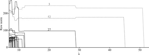
Arabidopsis thaliana data: outlier detection paths obtained by the robust reduced-rank regression. Sample 3 and sample 52 are captured as outliers, whose paths are shown as a dotted line and a dashed line, respectively. The path plot also suggests sample 27 as a potential outlier.

The low-rank model obtained reveals robust score variables, or factors, constructed from isoprenoid biosynthesis pathways, in response to the 62 genes in the four downstream pathways. Let $\tilde{X}$ denote the design matrix after removing the two detected outliers, and let $\widehat{U}\widehat{D}{\widehat{V}}^{\mathrm{T}}$ be the singular value decomposition of $\tilde{X}\widehat{B}$⁠. Then $\widehat{U}$ delivers five orthogonal factors, and $\widehat{V}\widehat{D}$ gives the associated factor coefficients. Figure 2 plots the coefficients of the first three leading factors for all 62 response variables. Given the $s$th factor (⁠$s=\mathrm{1,2}\mathrm{,3}$⁠), the genes are grouped into the four pathways separated by vertical lines, and two horizontal lines are placed at heights $\pm {\sigma }_s^{\tilde{X}\widehat{B}}{m}^{-1/2}$⁠. Therefore, the genes located beyond those two horizontal lines have relatively large-magnitude coefficients on the corresponding factor.

Fig. 2.

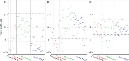
Arabidopsis thaliana data: factor coefficients of the 62 response genes from plastoquinone, carotenoid, phytosterol, and chlorophyll pathways. From left to right the panels correspond to the top three factors estimated by the robust reduced-rank regression. For the $s$th factor (⁠$s=\mathrm{1,2}\mathrm{,3}$⁠), two horizontal lines are plotted at heights $\pm {\sigma }_s^{\tilde{X}\widehat{B}}{m}^{-1/2}$⁠, and three vertical lines separate the genes into four different pathways.

We also tested the significance of the factors in response to each of the 62 genes; see Table 1. Plastoquinone was excluded since it has only two genes and its behaviour couples with that of carotenoid most of the time. Even with the familywise error rate controlled at $0.01$⁠, the factors obtained are predictive overall according to the significance percentages, although they play very different roles in different pathways. In fact, according to Fig. 2 and Table 1, the genes that are correlated with the first factor are mainly from carotenoid and chlorophyll, and almost all the coefficients there are negative. It seems that the first factor interprets some joint characteristics of carotenoid and chlorophyll; the second factor differentiates phytosterol genes from carotenoid genes; and the third factor appears to contribute mainly to the phytosterol pathway. Therefore, by projecting the data onto a proper low-dimensional subspace in a supervised and robust manner, distinct behaviours of the downstream pathways and their potential subgroup structures can be revealed. Further biological insights could be gained by closely examining the experimental and background conditions.

Table 1.

Arabidopsis thaliana data: percentage of genes on each response pathway that show significance of a given factor, with the familywise error rate controlled at level$0.01$

Pathway	Number of genes	Factor 1	Factor 2	Factor 3
Carotenoid	11	55%	73%	9%
Phytosterol	25	20%	48%	32%
Chlorophyl	24	75%	21%	0%

Acknowledgement

The authors thank the editor, associate editor and referees for suggestions that have significantly improved the paper. The first author thanks Art Owen for his valuable comments on an earlier version of the manuscript, and Elvezio Ronchetti for inspiration. This work was partially supported by the U.S. National Science Foundation, National Institutes of Health and Department of Defense.

Supplementary material

Supplementary material available at Biometrika online includes all technical details of the proofs, a financial example and the simulation studies.