Scalar-on-image regression via the soft-thresholded Gaussian process

Summary

This work concerns spatial variable selection for scalar-on-image regression. We propose a new class of Bayesian nonparametric models and develop an efficient posterior computational algorithm. The proposed soft-thresholded Gaussian process provides large prior support over the class of piecewise-smooth, sparse, and continuous spatially varying regression coefficient functions. In addition, under some mild regularity conditions the soft-thresholded Gaussian process prior leads to the posterior consistency for parameter estimation and variable selection for scalar-on-image regression, even when the number of predictors is larger than the sample size. The proposed method is compared to alternatives via simulation and applied to an electroencephalography study of alcoholism.

1. Introduction

Scalar-on-image regression has recently attracted considerable attention in both the frequentist and the Bayesian literature. This problem is challenging for several reasons: the predictor is a two-dimensional or three-dimensional image where the number of pixels or voxels is often larger than the sample size; the observed predictors may be contaminated with noise; the true signal may exhibit complex spatial structure; and most components of the predictor may have no effect on the response, and when they have an effect it may vary smoothly.

Regularized regression techniques are often needed when the number of predictors is much higher than the sample size. The lasso (Tibshirani, 1996) is a popular method for variable selection that employs a penalty based on the sum of the absolute values of the regression coefficients. However, most penalized approaches do not accommodate predictors with ordered components such as an image predictor. One exception is the fused lasso, which generalizes the lasso by penalizing both the coefficients and their successive differences and thus ensures both sparsity and smoothness of the estimated effect. To incorporate the spatial structure of the predictors, Reiss & Ogden (2010) extended functional principal component regression to handle image predictors by approximating the coefficient function using B-splines. However, this method is not sensitive to sparsity or sharp edges. Wang et al. (2017) proposed a penalty based on the total variation of the regression function that yields piecewise-smooth regression coefficients. The approach is focused primarily on prediction and does not quantify uncertainty in a way that permits statistical inference. Reiss et al. (2015) considered a wavelet expansion for the regression coefficients and conducted inference via hypothesis testing. Their approach requires that the image predictors have dimensions of equal size and moreover that the common size be a power of two. These strong assumptions are violated for our motivating application. Therefore, none of these methods are appropriate for detecting a piecewise-smooth, sparse, and continuous signal for a scalar outcome and an image predictor.

Scalar-on-image regression has been also approached from a Bayesian viewpoint. Goldsmith et al. (2014) proposed to model the regression coefficients as the product of two latent spatial processes to capture both sparsity and spatial smoothness of the important regression coefficients. They used an Ising prior for the binary indicator that a voxel is predictive of the response, and a conditionally autoregressive prior to smooth the nonzero regression coefficients. Use of an Ising prior for binary indicators was first discussed in Smith & Fahrmeir (2007) in the context of high-dimensional spatial predictors and was also recently employed by Li et al. (2015), who used a Dirichlet process prior for the nonzero coefficients. In both Li et al. (2015) and Goldsmith et al. (2014), sparsity and smoothness are controlled separately by two independent spatial processes, so the transitions from zero areas to neighbouring nonzero areas may be abrupt and computation is challenging because the Ising probability mass function does not have a simple closed form.

We propose an alternative approach to spatial variable selection in scalar-on-image regression by modelling the regression coefficients through soft-thresholding of a latent Gaussian process. The soft-thresholding function is well known for its relation with the lasso estimate when the design matrix is orthonormal (Tibshirani, 1996), and here we use it to specify a spatial prior with mass at zero. The idea is inspired by Boehm Vock et al. (2014), who considered Gaussian processes as a regularization technique for spatial variable selection. However, their approach does not assign prior probability mass at zero for regression coefficients and is not designed for scalar-on-image regression. Unlike other Bayesian spatial models (Goldsmith et al., 2014; Li et al., 2015), the soft-thresholded Gaussian process ensures a gradual transition between the zero and nonzero effects of neighbouring locations and provides large support over the class of spatially varying regression coefficient functions that are piecewise smooth, sparse, and continuous. The use of the soft-thresholded Gaussian process avoids the computational problems posed by the Ising prior, and can be scaled to large datasets using a low-rank spatial model for the latent process. We show that the soft-thresholded Gaussian process prior leads to posterior consistency for both parameter estimation and variable selection under mild regularity conditions, even when the number of predictors is larger than the sample size.

The proposed method is introduced for a single image predictor and Gaussian responses mainly for simplicity. Extensions to accommodate multiple predictors and non-Gaussian responses are relatively straightforward. However, the theoretical investigation of the procedure for non-Gaussian responses is not trivial, and so we establish the theory for binary responses and the probit link function. The methods are applied to data from an electroencephalography, EEG, study of alcoholism; see http://kdd.ics.uci.edu/datasets/eeg/eeg.data.html. The objective of our analysis is to estimate the relationship between alcoholism and brain activity. EEG signals are recorded for both alcoholics and controls at 64 channels of electrodes on subjects’ scalps for 256 seconds, leading to a high-dimensional predictor. The data have been previously described in Li et al. (2010) and Zhou & Li (2014). Previous literature has ignored the spatial structure of the electrodes shown in Fig. 1, which was recovered from the standard electrode position nomenclature described by Fig. 1 of https://www.acns.org/pdf/guidelines/Guideline-5.pdf. Our spatial analysis exploits the spatial configuration of the electrodes and reveals regions of the brain with activity predictive of alcoholism.

Fig. 1.

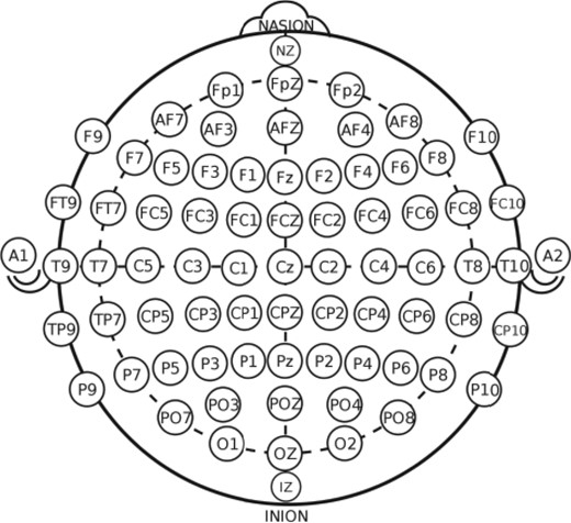
Standard electrode position nomenclature for the 10-10 system.

2. Model

2.1. Scalar-on-image regression

Let |${\mathbb R}^m$| be a |$m$|-dimensional vector space of real values. Suppose there are |$n$| subjects in the dataset and the data for subject |$i$| consist of a scalar response variable, |$Y_i\in{\mathbb R}^1$|⁠, a set of |$p_n$| spatially distributed image predictors, denoted by |${X}_i = (X_{i,1},\ldots, X_{i,p_n})^{{\rm T}} \in {\mathbb R}^{p_n}$|⁠, and other scalar covariates collected by |${W}_i = (W_{i,1},\ldots, W_{i,q})^{{\rm T}}\in{\mathbb R}^q$|⁠. Assume that |$\{{W}_i\}_{i=1}^n$| are fixed design covariates. Here |$X_{i,j}$| denotes the image intensity value measured at location |${s}_j$|⁠, for |$j = 1,\ldots, p_n$|⁠. We assume that the set of locations |${S} = \{{s}_j\}_{j=1}^{p_n}$| is a fixed subset of a compact closed region |${\cal B}\subseteq {\mathbb R}^d$|⁠. Let |${N}(\mu,\Sigma)$| denote a normal distribution with mean |$\mu$| and variance-covariance matrix |$\Sigma$|⁠, or variance for the one-dimensional case. We consider the scalar-on-image regression model

\begin{eqnarray}\label{eq:main_model} \ (Y_i \mid {W}_i, {X}_{i},{{\alpha}^{\rm v}}, \beta,\sigma^2\ ) \sim{N}\left\{\sum_{k=1}^q \alpha_{k} W_{i,k}+p_n^{-1/2}\sum_{j=1}^{p_n}\beta({s}_j) X_{i,j}, \sigma^2\right\} \quad (i = 1,\ldots, n), \end{eqnarray}

(1)

where |${{\alpha}^{\rm v}} = (\alpha_{1},\ldots,\alpha_{q})^{{\rm T}}$| quantifies the effect of |${W}_i$| and |$\beta(\cdot)$| is a spatially varying coefficient function defined on |${\cal B}$|⁠. In practice, the normalizing scalar |$p^{-1/2}_n$| can be absorbed into the image predictors; its role is to rescale the total effects of massive image predictors such that they are bounded away from infinity with large probability, when |$p_n$| is very large. Scientifically, in brain imaging studies, the image predictors take values that measure the body tissue contrast or the neural activities at each spatial location, and the number of image predictors, |$p_n$|⁠, is determined by the image resolution. Thus, the total effect of the image predictors reflects the total intensity in the brain signals, which should not increase to infinity as the image resolution increases. In model (1), the response is taken to be Gaussian and only one type of image predictor is included, although extensions of the modelling framework to non-Gaussian responses and multimodality image predictor regression are straightforward.

2.2. Soft-thresholded Gaussian processes

To capture the characteristics of the image predictors and their effects on the response variable, the prior for |$\beta(\cdot)$| should be sparse and spatial. That is, we assume that many locations have |$\beta({s}_j)=0$|⁠, the sites with nonzero coefficients cluster spatially, and the coefficients vary smoothly in clusters of nonzero coefficients. To encode these desired properties into the prior, we represent |$\beta(\cdot)$| as a transformation of a Gaussian process, |$\beta({s}) = g_{\lambda}\{\tilde \beta({s})\}$|⁠, where |$g_\lambda$| is the transformation function dependent on parameter |$\lambda$| and |$\tilde \beta({s})$| follows a Gaussian process prior. In this trans-kriging (Cressie, 1993) or Gaussian copula (Nelsen, 1999) model, the function |$g_\lambda$| determines the marginal distribution of |$\beta({s})$|⁠, while the covariance of the latent |$\tilde\beta({s})$| determines |$\beta({s})$|’s dependence structure.

Spatial dependence is determined by the prior for |$\tilde \beta({s})$|⁠. We assume that |$\tilde \beta(\cdot)$| is a Gaussian process with mean zero and stationary covariance function |$\mathrm{cov}\{\tilde \beta({s}), \tilde \beta ({s}')\} = \kappa({s}-{s}')$| for some covariance function |$\kappa$|⁠. Although other transformations are possible (Boehm Vock et al., 2014), we select |$g_\lambda$| to be the soft-thresholding function to map |$\tilde \beta({s})$| near zero to exact zero and thus give a sparse prior. Let

\begin{equation*}\label{beta} g_\lambda(x) = \left\{\begin{array}{@{}cl} 0, & |x|\leq \lambda,\\ {\mathrm{sgn}}(x)(|x|-\lambda), & |x|>\lambda, \end{array}\right. \end{equation*}

where |${\mathrm{sgn}}(x) = 1$| if |$x>0$|⁠, |${\mathrm{sgn}}(x) = -1$| if |$x<0$|⁠, and |${\mathrm{sgn}}(0) = 0$|⁠. The thresholding parameter |$\lambda>0$| determines the degree of sparsity. This soft-thresholded Gaussian process prior is denoted by |$\beta \sim {\small{\text{STGP}}}(\lambda,\kappa)$|⁠.

3. Theoretical properties

3.1. Notation and definitions

We first introduce additional notation for the theoretical development and the formal definitions of the class of spatially varying coefficient functions under consideration. We assume that all the random variables and stochastic processes in this article are defined on a probability space |$(\Omega, {\cal F}, \Pi)$|⁠. Let |$\mathbb{Z}^d_+ = \{0,1,\ldots \}^d \subset {\mathbb R}^d$| represent a space of |$d$|-dimensional nonnegative integers. For any vector |${v} = (v_1,\ldots, v_d)^{{\rm T}}\in {\mathbb R}^d$|⁠, let |$\|{v}\|_p = \big(\sum_{l=1}^d |v_l|^p\big)^{1/p}$| be the |$L_p$|-norm of vector |${v}$| for any |$p\geq 1$|⁠, and let |$\|{v}\|_\infty = \max_{l=1}^d |v_l|$| be the supremum norm. For any |$x\in {\mathbb R}$|⁠, let |$\lceil x \rceil$| be the smallest integer not smaller than |$x$| and let |$\lfloor x \rfloor$| be the largest integer not larger than |$x$|⁠. Define the event indicator |$I({\cal A})=1$| if event |${\cal A}$| occurs and |$I({\cal A}) = 0$| otherwise. For any |${z} = (z_1,\ldots, z_d)^{{\rm T}} \in \mathbb{Z}^d_+$|⁠, define |${z} ! = \prod_{l=1}^d \prod_{k=1}^{z_l} k$| and |${v}^{{z}} = \prod_{l=1}^d v_l^{z_l}$|⁠. For any real function |$f$| on |${\cal B}$|⁠, let |$\|f\|_p = \left\{\int_{{\cal B}}|f({s})|^p\,{\rm d} {s}\right\}^{1/p}$| denote the |$L_p$|-norm for any |$p\geq 1$| and let |$\|f\|_{\infty} = \sup_{{s}\in{\cal B}}|f({s})|$| denote the supremum norm.

 

Definition 1.

Denote by |${\mathcal C}^{m}({\cal B})$| the set of differentiable functions |$f(\cdot)$| of order |$m$| defined on |${\cal B}$| such that |$f({s})$| has partial derivatives

$$D^{{\tau}} f({s}) = \frac{\partial^{\|{\tau}\|_1}f}{s_1^{\tau_1}\cdots s_d^{\tau_d}}({s}) = \sum_{\|{\eta}\|_1 + \|{\tau}\|_1\leq m} \frac{D^{{\tau}+{\eta}}f({t})}{{\eta}!}({s}-{t})^{{\eta}} + R_m({s},{t}),$$

where |${\tau} = (\tau_1, \ldots, \tau_d)^{{\rm T}}\in \mathbb {Z}_+^{d}$|⁠, |${\eta}\in\mathbb{Z}_+^{d}$| and |${t} \in {\mathbb R}^d$| and given any point |${s}_0$| of |${\cal B}$| and any |$\varepsilon >0$|⁠, there is a |$\delta>0$| such that if |${s}$| and |${t}$| are any two points of |${\cal B}$| with |$\|{s}-{s}_0\|_1<\delta$| and |$\|{t}-{s}_0\|_1<\delta$|⁠, then |$|R_m({s},{t})|\leq \|{s}-{t}\|_1^{m-\|{\tau}\|_1}\varepsilon$|⁠. If |$\|D^{{\tau}}f\|_\infty \leq M <\infty$|⁠, then |$|R_m({s},{t})|\leq (M\|{s}-{t}\|_1^{m+1})/(m+1)!$|.

Denote by |$\bar {\cal R}$| and |$\partial {\cal R}$| the closure and the boundary of any set |${\cal R}\subseteq {\cal B}$|⁠.

 

Definition 2.

Define |$\Theta = \{\beta({s}): {s}\in{\cal B}\}$| to be the collection of all spatially varying coefficient functions that satisfy the following conditions. Assume that there exist two disjoint nonempty open sets |${\cal R}_{-1}$| and |${\cal R}_{1}$| with |$\bar {\cal R}_1 \cap \bar {\cal R}_{-1} = \emptyset$| such that:

• (i) |$\beta(\cdot)$| is smooth over |$\bar {\cal R}_{-1}\cup \bar {\cal R}_{1}$|⁠, i.e.,

  $$\beta({s})I({s}\in \bar {\cal R}_{-1} \cup \bar {\cal R}_{1})\in {\mathcal C}^\rho(\bar {\cal R}_{-1}\cup \bar {\cal R}_{1}),\qquad \rho = \lceil d/2 \rceil\text{;}$$

• (ii) |$\beta({s})=0$| for |${s}\in {\cal R}_0$|⁠, |$\beta({s})>0$| for |${s}\in {\cal R}_1$| and |$\beta({s})<0$| for |${s}\in {\cal R}_{-1}$|⁠, where |${\cal R}_0 = {\cal B} - ({\cal R}_{-1}\cup {\cal R}_1)$| and |${\cal R}_0-(\partial {\cal R}_1 \cup \partial {\cal R}_{-1})\neq \emptyset$|;

• (iii) |$\beta(\cdot)$| is continuous over |${\cal B}$|⁠, i.e., |$\lim_{{s}\rightarrow {s}_0}\beta({s}) = \beta({s}_0) \qquad ({s}_0 \in {\cal B})\text{.}$| 

Simply put, |$\Theta$| is the collection of all piecewise-smooth, sparse and continuous functions defined on |${\cal B}$|⁠.

3.2. Large support

One desirable property for the Bayesian nonparametric model is that it should have prior support over a large class of functions. In this section, we show that the soft-thresholded Gaussian process has large support over |$\Theta$|⁠. We begin with two appealing properties of the soft-thresholding function. All technical conditions are listed in the Appendix, as Conditions A1–A5.

 

Lemma 1.

The soft-thresholding function |$g_\lambda(x)$| is Lipschitz continuous for any |$\lambda > 0$|⁠, that is, for all |$x_1, x_2 \in {\mathbb R}$|⁠, |$|g_\lambda (x_1)-g_\lambda (x_2)| \leq |x_1 - x_2|\text{.}$| 

 

Lemma 2.

For any function |$\beta_0\in\Theta$| and any threshold parameter |$\lambda_0>0$|⁠, there exists a smooth function |$\tilde\beta_0({s})\in {\mathcal C}^{\rho}({\cal B})$| such that |$\beta_0({s}) = g_{\lambda_0}\{\tilde\beta_0({s})\}\text{.}$| 

Lemma 1 is proved directly by verifying the definition. The proof of Lemma 2 is not trivial, it requires a detailed construction of the smooth function |$\tilde\beta_0({s})$|⁠. See the Appendix for details.

 

Theorem 1.

For any function |$\beta_0 \in \Theta$| and |$\varepsilon>0$|⁠, the soft-thresholded Gaussian process prior |$\beta \sim{\small{\text{STGP}}}(\lambda_0, \kappa)$| satisfies |$\Pi\left(\|\beta-\beta_0\|_{\infty}<\varepsilon\right)>0$|⁠, for any |$\lambda_0>0$| and |$\kappa$| that satisfy Condition A5.

 

Proof.

By Lemma 2, for any threshold parameter |$\lambda_0>0$| there is a smooth function |$\tilde\beta_0({s})\in {\mathcal C}^{\rho}({\cal B})$| such that |$\beta_0({s}) = g_{\lambda_0}\{\tilde\beta_0({s})\}$|⁠. Since |$\beta\sim {\small{\text{STGP}}}(\lambda_0,\kappa)$|⁠, we have |$\beta({s}) = g_{\lambda_0}\{\tilde\beta({s})\}$| with |$\tilde\beta({s}) \sim {\cal GP}(0, \kappa),$| By Lemma 1,

\begin{eqnarray*} \Pi\left\{\sup_{{s}\in {\cal B}}|\beta({s})-\beta_0({s})|<\varepsilon\right\}&=&\Pi\left[\sup_{{s}\in {\cal B}}|g_{\lambda_0}\{\tilde\beta({s})\}-g_{\lambda_0}\{\tilde\beta_0({s})\}|<\varepsilon\right]\\ &\geq& \Pi\left\{\sup_{{s}\in {\cal B}}|\tilde\beta({s})-\tilde\beta_0({s})|<\varepsilon\right\}\!\text{.} \end{eqnarray*}

By Condition A5 and Theorem 4|$\cdot$|5 of Tokdar & Ghosh (2007), |$\tilde\beta_0(\cdot)$| is in the reproducing kernel Hilbert space of |$\kappa$|⁠, and then by Theorem 4 of Ghosal & Roy (2006) we have |$\Pi\left\{\sup_{{s}\in {\cal B}}|\tilde\beta({s})-\tilde\beta_0({s})|<\varepsilon\right\}>0$|⁠, which completes the proof. □

Theorem 1 implies that there is always a positive probability that the soft-thresholded Gaussian process concentrates in an arbitrarily small neighbourhood of any spatially varying coefficient function that has piecewise smoothness, sparsity and continuity properties. According to Lemma 2, for any positive |$\lambda_1 \neq \lambda_2$|⁠, there exist |$\tilde\beta_1,\tilde\beta_2 \in{\mathcal C}^{\rho}({\cal B})$| such that |$\beta_0({s}) = g_{\lambda_1}\{\tilde\beta_1({s})\} = g_{\lambda_2}\{\tilde\beta_2({s})\}$|⁠. Thus the thresholding parameter |$\lambda_0$| and the latent smooth curve |$\tilde \beta_0$| are not identifiable, but we can ensure that |$\beta_0$| is identifiable by establishing the posterior consistency of parameter estimation.

3.3. Posterior consistency

For |$i = 1,\ldots, n$|⁠, given the image predictor |${X}_i$| on a set of spatial locations |${S}$| and other covariates |${W}_i$|⁠, suppose that the response |$Y_i$| is generated from the scalar-on-image regression model (1) with parameters |${{\alpha}^{\rm v}_0}\in {\mathbb R}^{q}$|⁠, |$\sigma^2_0>0$| and |$\beta_0 \in\Theta$|⁠. For theoretical convenience we assume that |${{\alpha}^{\rm v}_0}$| and |$\sigma^2_0$| are known; in practice it is straightforward to estimate them from the data. We assign a soft-thresholded Gaussian process prior for the spatially varying coefficient function, i.e., |$\beta \sim {\small{\text{STGP}}}(\lambda, \kappa)$| for any given |$\lambda>0$| and covariance kernel |$\kappa$|⁠. In light of the large-support property in Theorem 1, the following lemma shows the positivity of prior neighbourhoods.

 

Lemma 3.

Denote by |$\pi_{n,i}(\cdot; \beta)$| the density function of |${Z}_{n,i} = (Y_i,{W}_i,{X}_{i})$| in model (1) and suppose that Condition A4 holds for |${X}_i$|⁠. Define |$\Lambda_{n,i}(\cdot; \beta_0,\beta) = \log \pi_{n,i}(\cdot; \beta) - \log \pi_{n,i}(\cdot; \beta_0)$|⁠, |$K_{n,i}(\beta_0,\beta) = {E}_{\beta_0} \{\Lambda_{n,i}({Z}_{n,i}; \beta_0,\beta)\}$| and |$V_{n,i}(\beta_0,\beta) = {\rm Var}_{\beta_0} \{\Lambda_{n,i}({Z}_{n,i}; \beta_0,\beta)\}$|⁠. There exists a set |$B$| with |$\Pi(B)>0$| such that, for any |$\varepsilon > 0$|,

\begin{eqnarray*} \liminf_{n\rightarrow\infty} \Pi\left[\left\{\beta\in B, n^{-1}\sum_{i=1}^n K_{n,i}(\beta_0,\beta)<\varepsilon\right\}\right] > 0, \quad n^{-2} \sum_{i=1}^n V_{n,i}(\beta_0,\beta) \rightarrow 0,\quad \beta \in B\text{.} \end{eqnarray*}

We construct sieves for the spatially varying coefficient functions in |$\Theta$| as

\begin{equation*}\label{eq:sieve} \Theta_n = \left\{\beta \in\Theta: \|\beta\|_\infty \leq p_n^{1/(2d)}, \sup_{{s} \in {\cal R}_1\cup {\cal R}_{-1}}|D^{{\tau}}\beta({s})| \leq p_n^{1/(2d)}, 1\leq\|{\tau}\|_1 \leq \rho \right\}\!, \end{equation*}

where |$\rho$| is defined in Condition A1. By Lemmas A1–A5 in the Appendix, we can find an upper bound for the tail probability and construct uniform consistent tests in the following lemmas.

 

Lemma 4.

If |$\beta({s})\sim {\small{\text{STGP}}}(\lambda_0,\kappa)$| with |$\lambda_0>0$| and the kernel function |$\kappa$| satisfies Condition A5, then there exist constants |$K$| and |$b$| such that for all |$n\geq 1$|⁠, |$\Pi(\Theta_n^C) \leq K \exp(-b p_n^{1/d})\text{.}$| 

 

Lemma 5.

For any |$\varepsilon>0$| and |$\upsilon_0/2<\upsilon<1/2$|⁠, there exist |$N$|⁠, |$C_0$|⁠, |$C_1$| and |$C_2$| such that for all |$n>N$| and all |$\beta \in \Theta_n$|⁠, if |$\|\beta - \beta_0\|_1>\varepsilon$|⁠, a test function |$\Psi_n$| can be constructed such that |${E}_{\beta_0}(\Psi_n) \leq C_{0}\exp(-C_{2} n^{2\upsilon})$| and |${E}_{\beta}(1-\Psi_n) \leq C_{0} \exp\left(-C_{1} n\right)$|⁠, where |$\upsilon_0$| is defined in Condition A1.

Proofs of Lemmas 3–5 are provided in the Supplementary Material. These lemmas verify three important conditions for proving posterior consistency in the scalar-on-image regression based on Theorem A1 of Choudhuri et al. (2004). Thus we have the following theorem.

 

Theorem 2.

Denote the data by |${D}_n = \{Y_i, {X}_i, {W}_i\}_{i=1}^n$|⁠. If Conditions A1–A5 hold, then for any |$\varepsilon>0$|,

\begin{equation}\label{eq:post_consistency} \Pi\left(\beta\in\Theta: \|\beta-\beta_0\|_1<\varepsilon \mid{D}_n \right) \to 1, \quad n\to\infty\text{.} \end{equation}

(2)

Theorem 2 implies that the soft-thresholded Gaussian process prior can ensure that the posterior distribution of the spatially varying coefficient function concentrates in an arbitrarily small neighbourhood of the true value, when the numbers of subjects and spatial locations are both sufficiently large. Given that the true function of interest is piecewise smooth, sparse and continuous, the soft-threshold Gaussian process prior can further ensure that the posterior probability of the sign of the spatially varying coefficient function being correct converges to 1 as the sample size goes to infinity. The result is formally stated in the following theorem.

 

Theorem 3.

Suppose that the model assumptions, prior settings and regularity conditions for Theorem 2 hold. Then

\begin{equation}\label{eq:sign_consistency} \Pi\left[ {\mathrm{sgn}}\{\beta({s})\} = {\mathrm{sgn}}\{\beta_0({s})\}, \ {s}\in {\cal B} \mid {D}_n\right] \to 1, \qquad n \to\infty\text{.} \end{equation}

(3)

This theorem establishes the consistency of spatial variable selection. It does not require that the number of true image predictors be finite or less than the sample size. This result is reasonable in that the true spatially varying coefficient function is piecewise smooth and continuous, and the soft-thresholded Gaussian process will borrow strength from neighbouring locations to estimate the true image predictors. The Supplementary Material gives proofs of Theorems 2 and 3.

To apply the proposed model to the motivating dataset, we extend the proposed model (1) and Theorems 2 and 3 to analysis of the binary response variable using a probit model:

\begin{eqnarray}\label{eq:probit_model} Y_i \sim{\rm Ber}(\pi_i),\quad \Phi^{-1}(\pi_i)= \sum_{k=1}^q \alpha_{k} W_{i,k}+p_n^{-1/2}\sum_{j=1}^{p_n}\beta({s}_j) X_{i,j}, \end{eqnarray}

(4)

where |$\Phi(\cdot)$| is the standard normal cumulative distribution function.

 

Theorem 4.

Assume that the data |${D}_n$| are generated from model (4) and prior settings are the same as in Theorem 2. If Conditions A1–A5 and S|$1$|–S|$3$|hold, then (2) and (3) hold under model (4).

Conditions S1–S3 and the proof of Theorem 4 are in the Supplementary Material.

4. Posterior computation

4.1. Model representation and prior specification

Next, we discuss the practical applicability of our method. We select a low-rank spatial model to ensure that computation remains possible for large datasets, and exploit the kernel convolution approximation of a spatial Gaussian process. As discussed in Higdon et al. (1999), any stationary Gaussian process |$V({s})$| can be written as |$V({s}) = \int K({s}-{t})w({t})\,{\rm d}{t}$|⁠, where |$K$| is a kernel function and |$w$| is a white-noise process with mean zero and variance |$\sigma_w^2$|⁠. Then the covariance function of |$V(\cdot)$| is |$\mbox{cov}\{V({s}),V({s}+{h})\} = \kappa({h})=\sigma_a^2\int K({s}-{t})K({s}+{h}-{t})\,{\rm d}{t}$|⁠.

This representation suggests the following approximation for the latent process |$\tilde\beta({s}) \approx \sum_{l=1}^LK({s}-{t}_l)a_l \delta,$| where |${t}_1,\ldots,{t}_L\in{\mathbb R}^d$| are a grid of equally spaced spatial knots covering |${\cal B}$| and |$\delta$| is the grid size. Without loss of generality, we assume that |$\delta = 1$| and |$K$| is a local kernel function. We use tapered Gaussian kernels with bandwidth |$\sigma_h$|⁠, |$K(h) = \exp\{-h^2/(2\sigma_h)^2\}I(h<3\sigma_h)$|⁠, so that |$K(\|{s}-{t}_l\|)=0$| for |${s}$| separated from |${t}_l$| by at least |$3\sigma_h$|⁠. Taking |$L<p$| knots and selecting compact kernels leads to computational savings, as discussed in § 4.2.

The compact kernels |$K$| control the local spatial structure and the prior for the coefficients |${a} = (a_1,\ldots,a_L)^{{\rm T}}$| controls the broad spatial structure. Following Nychka et al. (2015), we assume that the knots |${t}_1,\ldots,{t}_L$| are arranged on an |$m_1 \times \cdots \times m_d$| array, and use |$l\sim k$| to denote that knots |${t}_l$| and |${t}_k$| are adjacent on this array. We then use a conditionally autoregressive prior (Gelfand et al., 2010) for the kernel coefficients. The conditional autoregressive prior is also defined locally, with full conditional distribution

\begin{equation}\label{CR} a_l \mid a_k, k\neq l \sim \mbox{N}\left(\frac{\vartheta}{n_l}\sum_{k\sim l}a_k, \frac{\sigma_a^2}{n_l}\right)\!, \end{equation}

(5)

where |$n_l$| is the number of knots adjacent to the knot |$l$|⁠, |$\vartheta\in(0,1)$| quantifies the strength of spatial dependence, and |$\sigma_a^2$| determines the variance. These full conditional distributions correspond to the joint distribution |${a} \sim N\{0,\sigma_a^2({M}-\vartheta {A})^{-1}\}$|⁠, where |${M}$| is diagonal with diagonal elements |$(n_1,\ldots,n_L)$| and |${A}$| is the adjacency matrix with |$(k,l)$| element equal to 1 if |$k\sim l$| and zero otherwise.

Write |${\tilde{\beta}}^{\rm v} = \{\tilde\beta({s}_1),\ldots,\tilde\beta({s}_p)\}^{{\rm T}}$|⁠. Denote by |${K}$| the |$p\times L$| kernel matrix with |$(j,l)$| element |$K(\|{s}_j-{t}_l\|_{2})$|⁠; then |$\tilde{{\beta}^{\rm v}} \sim {N}\{0,\sigma_a^2{K}({M}-\vartheta{A})^{-1}{K}^{{\rm T}}\}$| as a prior distribution. In this case, the |$\tilde\beta({s}_j)$| do not have equal variances, which may be undesirable. Nonconstant variance arises because the kernel knots may be unequally distributed, and because the conditional autoregressive model is nonstationary in that the variances of the |$a_l$| are unequal.

To stabilize the prior variance, define |${\tilde K}_{j,l} = K(\|{s}_j-{t}_l\|_2)/w_{j}$| and let |${\tilde K}$| be the corresponding |$p\times L$| matrix of standardized kernel coefficients, where |$w_j$| are constants chosen so that the prior variance for |$\beta_j$| is the same over |$j$|⁠. We take |$w_j$| to be the square root of the |$j$|th diagonal element of |${K}({M}-\vartheta {A})^{-1}{K}^T$|⁠, so the kernel functions depend on |$\vartheta$|⁠. By pulling the prior standard deviation |$\sigma_a$| out of the thresholding transformation, we have an equivalent representation of (1) as

\begin{equation}\label{beta2} Y_i \sim{N}({W}_i^{{\rm T}}{{\alpha}^{\rm v}} + p^{-1/2}_n{X}_i^{{\rm T}}{{\beta}^{\rm v}},\sigma^2),\qquad \beta({s}_j) = \sigma_a g_\lambda\{\tilde\beta({s}_j)\}, \end{equation}

(6)

where |${\tilde{\beta}}^{\rm v}\sim {N}\{0,\tilde{K}({M}-\vartheta{A})^{-1}\tilde{K}^{{\rm T}}\}$|⁠. After standardization, the prior variance of each |$\tilde\beta({s}_j)$| is 1, and therefore the prior probability that |$\tilde \beta({s}_j)$| is nonzero is |$2\Phi(-\lambda)$| for all |$j$|⁠. This endows each parameter with a distinct interpretation: |$\sigma_a$| controls the scale of the nonzero coefficients, |$\lambda$| controls the prior degree of sparsity, and |$\vartheta$| controls spatial dependence. With an additional set of conditions, we can show that model representation (6) when |$L\to\infty$| has a large prior support, thus leading to the posterior consistency and selection consistency. The Supplementary Material contains more details.

In practice, we normalize the response and covariates, and then select priors |${{\alpha}^{\rm v}}\sim N (0,10^2 \mathrm{I}_q)$|⁠, |$\sigma^2\sim {\small{\text{IG}}}($|0|$\cdot$|1, 0|$\cdot$|1|$)$|⁠, |$\sigma_a\sim \mbox{HalfNormal}(0,1)$|⁠, |$\vartheta\sim\mbox{Be}(10,1)$|⁠, and |$\lambda\sim\mbox{Un}(0,5)$|⁠. Following Banerjee et al. (2004), we use a beta prior for |$\vartheta$| with mean near one because only values near one provide appreciable spatial dependence. Finally, although our asymptotic results suggest that any |$\lambda>0$| will give posterior consistency, in finite samples posterior inference may be sensitive to the threshold and so we use a prior rather than a fixed value.

4.2. Markov chain Monte Carlo algorithm

For fully Bayesian inference on model (1), we sample from the posterior distribution using Metropolis–Hastings within Gibbs sampling. The parameters |${{\alpha}^{\rm v}}$|⁠, |$\sigma^2$|⁠, and |$\sigma^2_a$| have conjugate full conditional distributions and are updated using Gibbs sampling. The spatial dependence parameter |$\vartheta$| is sampled with Metropolis–Hastings sampling using a beta candidate distribution with the current value as mean and standard deviation tuned to give an acceptance rate of around 0|$\cdot$|4. The threshold |$\lambda$| is updated using Metropolis sampling with a random-walk Gaussian candidate distribution with standard deviation tuned to have acceptance probability around 0|$\cdot$|4. The Metropolis update for |$a_l$| uses the prior full conditional distribution in (5) as the candidate distribution, which gives a high acceptance rate and thus good mixing without tuning.

To make posterior inference for the probit regression model (4), we can slightly modify the aforementioned algorithm by introducing an auxiliary continuous variable |$Y_i^{*}$| for each response variable |$Y_i$|⁠. We assume that |$Y_i = I(Y_i^* > 0)$| and |$Y^*_i$| follows (1) with |$\sigma^2 = 1$|⁠. The full conditional distribution of |$Y^*_i$| is truncated normal and is straightforward to generate as a Gibbs sampling step in the posterior computation. The updating schemes for other parameters remain the same. For other types of non-Gaussian response models, we can use Metropolis–Hastings sampling directly by modifying the likelihood function accordingly.

5. Simulation study

5.1. Data generation

In this section we conduct a simulation study to compare the proposed methods with other popular methods for scalar-on-image regression. For each simulated observation, we generate a two-dimensional image |${X}_i$| on the |$\{1,\ldots,m\}\times \{1,\ldots, m\}$| grid with |$m=30$|⁠. The covariates are generated following two covariance structures: exponential, and having shared structure with the signal. The exponential covariates are Gaussian with mean |$E(X_{ij})=0$| and cov|$(X_{i,j},X_{i,l}) = \exp(-d_{j,l}/\vartheta_x)$|⁠, where |$d_{j,l}$| is the distance between locations |$j$| and |$l$| and |$\vartheta_x$| controls the range of spatial dependence. The covariates generated with shared structure with |${{\beta}^{\rm v}}$| are |${X}_i = {\tilde {X}}_i/2 + e_i{{\beta}^{\rm v}}$|⁠, where |${\tilde {X}}_i$| is Gaussian with exponential covariance with |$\vartheta_x=3$| and |$e_i \sim {N}(0,\upsilon^2)$|⁠. The continuous response is then generated as |$Y_i\sim N({X}_i^{{\rm T}}{{\beta}^{\rm v}},\sigma^2)$|⁠, and the binary response as |$Y_i\sim{\rm Ber}(\pi_i)$| with |$\Phi^{-1}(\pi_i) = {X}_i^{{\rm T}}{{\beta}^{\rm v}}$|⁠. Both |${X}_i$| and |$Y_i$| are independent for |$i=1,\ldots,n$|⁠. We consider three true |${{\beta}^{\rm v}}$| images: two sparse images plotted in Fig. 2, five peaks and triangle, and the dense image waves with |$\beta(s) = \{\cos(6\pi s_1/m) + \cos(6\pi s_2/m)\}/5$|⁠. We also compare sample size |$n\in\{100,250\}$|⁠, spatial correlation |$\vartheta_x\in\{3,6\}$|⁠, and error standard deviation |$\sigma\in\{2,5\}$|⁠. For all combinations of these parameters considered we generate |$S=100$| datasets. We also simulate binary data with |$\Pi(Y_i=1) = \Phi({X}_i^{{\rm T}}{{\beta}^{\rm v}})$| with |$n=250$| and exponential covariance with |$\vartheta_x=3$|⁠.

Fig. 2.

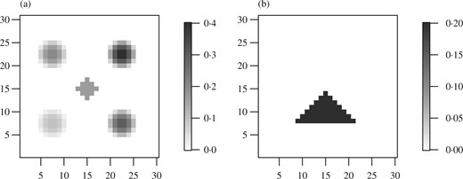
True |${{\beta}^{\rm v}}$| images used in the simulation study: (a) Five peaks; (b) Triangle.

5.2. Methods

We fit our model with an |$m/2 \times m/2$| equally spaced grid of knots covering |$\{1,\ldots,m\}\times \{1,\ldots, m\}$| with bandwidth |$\sigma_h$| set to the minimum distance between knots. We fit our model both with |$\lambda>0$|⁠, where the prior is a soft-thresholded Gaussian process with sparsity, and with |$\lambda=0$|⁠, in which case the prior is a Gaussian process with no sparsity. For both models, we run the proposed Markov chain Monte Carlo algorithm for 50 000 iterations with a 10 000-iteration burn-in, and compute the posterior mean of |${{\beta}^{\rm v}}$|⁠. For the sparse model, we compute the posterior probability of a nonzero |$\beta({s})$|⁠.

We compare our method with the lasso (Tibshirani, 1996) and fused lasso (Tibshirani et al., 2005; Tibshirani & Taylor, 2011) penalized regression estimates

\begin{eqnarray*}\label{fused} {\hat{\beta}_{\mathrm{L}}^{\mathrm{v}}} &=& \underset{{{\beta}^{\rm v}}}{\operatorname{arg\,min}}\left\{ ({Y} - {X}{{\beta}^{\rm v}})^{{\rm T}}({Y}-{X}{{\beta}^{\rm v}}) + \tilde\lambda\sum_j|\beta({s}_j)|\right\}\!, \\ {\hat{\beta}_{\mathrm{FL}}^{\mathrm{v}}} &=& \underset{{{\beta}^{\rm v}}}{\operatorname{arg\,min}}\left\{ ({Y} - {X}{{\beta}^{\rm v}})^{{\rm T}}({Y}-{X}{{\beta}^{\rm v}}) +\tilde\lambda\sum_{j\sim k}|\beta({s}_j)-\beta({s}_k)| + \tilde\gamma\tilde\lambda\sum_j|\beta({s}_j)|\right\}\!\text{.}\nonumber \end{eqnarray*}

The lasso estimate |${\hat{\beta}_{\mathrm{L}}^{\mathrm{v}}}$| is computed using the lars package (Hastie & Efron, 2013) in R (R Core Team, 2018), and the tuning parameter |$\tilde\lambda$| is selected using the Bayesian information criterion. The fused lasso estimate |${\hat{\beta}_{\mathrm{FL}}^{\mathrm{v}}}$| is computed using the genlasso package (Arnold & Tibshirani, 2014) in R. The fussed lasso has two tuning parameters: |$\tilde\gamma$| and |$\tilde\lambda$|⁠. Owing to computational considerations, we search only over |$\tilde\gamma$| in |$\{1/5,1,5\}$|⁠. For each |$\tilde\gamma$|⁠, |$\tilde\lambda$| is selected using the Bayesian information criterion. The Supplementary Material gives results for each |$\tilde\gamma$|⁠; here we report only the results for the |$\tilde\gamma$| with the most precise estimates.

We also consider a functional principal component analysis-based alternative. We smooth each image using the technique of Xiao et al. (2013) implemented in the fbps function in R’s refund package (Crainiceanu et al., 2014), compute the eigendecomposition of the sample covariance of the smoothed images, and then perform principal components regression using the lasso penalty tuned via the Bayesian information criterion. The Supplementary Material gives results using the leading eigenvectors that explain 80%, 90%, and 95% of the variation in the sample images, and here we report only the results for the value with the most precise estimates.

Finally, we compare our approach with the Bayesian spatial model of Goldsmith et al. (2014) using |$\beta({s}_j) = \tilde\alpha_j\theta_j$|⁠, where |$\tilde\alpha_j\in\{0,1\}$| is the binary indicator that location |$j$| is included in the model, and |$\theta_j\in {\mathbb R}$| is the regression coefficient given that the location is included. Both the |$\tilde\alpha_j$| and the |$\theta_j$| have spatial priors; the continuous components |$\theta_j$| follow a conditional autoregressive prior, and the binary components |$\alpha_j$| follow an Ising or autologistic prior (Gelfand et al., 2010) with full conditional distributions,

\begin{equation*}\label{autologistic} \mathrm{logit}~\Pi(\tilde\alpha_j = 1 \mid \tilde\alpha_l, l\neq j)= a_0 + b_0\sum_{l\sim j}\tilde\alpha_l\text{.} \end{equation*}

Estimating |$a_0$| and |$b_0$| is challenging because of the complexity of the Ising model (Møller et al., 2006), so Goldsmith et al. (2014) recommended selecting |$a_0$| and |$b_0$| using crossvalidation over |$a_0\in (-4,0)$| and |$b_0\in(0,2)$|⁠. For computational reasons we select values in the middle of these intervals and set |$a_0=-2$| and |$b_0=1$|⁠. The posterior mean of |$\beta({s})$| and the posterior probability of a nonzero |$\beta({s})$| are approximated based on 5000 Markov chain Monte Carlo samples after the first 1000 are discarded as burn-in.

5.3. Results

Tables 1 and 2 give the mean squared error for |${{\beta}^{\rm v}}$| estimation averaged over location, Type I error and power for detecting nonzero signals, and the computing time. The soft-thresholded Gaussian process model gives the smallest mean squared error when the covariate has exponential correlation. Compared to the Gaussian process model, adding thresholding reduces mean squared error by roughly 50% in many cases. As expected, the functional principal component analysis method gives the smallest mean squared error in the shared-structure scenarios where the covariates are generated to have a similar spatial pattern to the true signal. Even in this case, the proposed method outperforms other methods that do not exploit this shared structure. Under the dense waves signal the nonsparse Gaussian process model gives the smallest mean squared error, but the proposed method remains competitive.

Table 1.

Simulation study results for linear regression models. Methods are compared in terms of mean squared error for |${{\beta}^{\rm v}}$|⁠, Type I error and power for feature detection. The scenarios vary by the true |${{\beta}^{\rm v}}_0$|⁠, sample size |$n$|⁠, similarity between covariates and true signal determined by |$\tau$|⁠, error variance |$\sigma$|⁠, and spatial correlation range of the covariates |$\vartheta_x$|⁠. Results are reported as the mean with the standard deviation in parentheses over the |$100$| simulated datasets 

					Mean squared error for |${{\beta}^{\rm v}}$|⁠, multiplied by |$10^4$|
Signal	|$n$|	|$\tau$|	|$\sigma$|	|$\vartheta_x$|	Lasso	Fused lasso	FPCA	Ising	GP	STGP
Five peaks	100	0	5	3	326 (5)	22 (0)	36 (0)	46 (1)	27 (0)	13 (0)
	100	0	5	6	553 (9)	22 (0)	33 (0)	44 (1)	28 (0)	13 (0)
	100	0	2	3	102 (1)	11 (0)	24 (0)	26 (0)	15 (0)	4 (0)
	250	0	5	3	674 (9)	13 (0)	27 (0)	52 (1)	17 (0)	6 (0)
Triangle	100	0	5	3	289 (4)	9 (0)	17 (0)	30 (1)	19 (0)	8 (0)
	100	0	5	6	515 (9)	8 (0)	1|$\cdot$|5 (0)	28 (1)	19 (0)	8 (0)
	100	0	2	3	73 (1)	5 (0)	12 (0)	14 (0)	10 (0)	4 (0)
	250	0	5	3	650 (9)	6 (0)	14 (0)	34 (0)	12 (0)	6 (0)
	100	2	5	3	1011 (17)	7 (0)	10 (0)	27 (1)	33 (1)	13 (1)
	100	4	5	3	1018 (17)	6 (0)	4 (1)	32 (1)	34 (1)	14 (1)
Waves	100	0	5	3	1260 (13)	250 (5)	188 (7)	419 (3)	48 (1)	109 (10)
	100	0	5	6	1639 (17)	233 (4)	126 (3)	402 (4)	51 (1)	128 (12)

					Type I error, %				Power, %
Signal	|$n$|	|$\tau$|	|$\sigma$|	|$\vartheta_x$|	Lasso	Fused lasso	Ising	STGP	Lasso	Fused lasso	Ising	STGP
Five peaks	100	0	5	3	10 (0)	14 (1)	0 (0)	4 (1)	17 (0)	55 (2)	4 (0)	51 (1)
	100	0	5	6	10 (0)	37 (1)	0 (0)	7 (1)	15 (0)	80 (1)	5 (0)	58 (1)
	100	0	2	3	79 (0)	24 (1)	0 (0)	4 (1)	28 (0)	84 (1)	4 (0)	82 (1)
	250	0	5	3	27 (0)	19 (1)	0 (0)	4 (1)	32 (0)	77 (1)	10 (0)	71 (1)
Triangle	100	0	5	3	10 (0)	5 (0)	0 (0)	4 (1)	23 (1)	85 (1)	9 (0)	87 (1)
	100	0	5	6	11 (0)	8 (1)	0 (0)	4 (1)	19 (1)	91 (1)	9 (0)	86 (1)
	100	0	2	3	9 (0)	7 (1)	0 (0)	4 (0)	42 (1)	95 (0)	5 (0)	98 (0)
	250	0	5	3	27 (0)	5 (0)	0 (0)	4 (0)	35 (1)	92 (1)	16 (0)	96 (1)
	100	2	5	3	11 (0)	7 (1)	0 (0)	1 (0)	17 (0)	86 (1)	8 (0)	70 (1)
	100	4	5	3	11 (0)	2 (1)	0 (0)	3 (1)	19 (1)	84 (1)	12 (0)	73 (1)

					Computing time, minutes
Signal	|$n$|	|$\tau$|	|$\sigma$|	|$\vartheta_x$|	Lasso	Fused lasso	FPCA	Ising	GP	STGP
Five peaks	100	0	5	3	0|$\cdot$|02	16|$\cdot$|77	5|$\cdot$|40	27|$\cdot$|61	4|$\cdot$|81	11|$\cdot$|28

Type I error, proportion of times that zero coefficients were estimated to be nonzero; Power, proportion of times that nonzero coefficients were estimated to be nonzero; FPCA, functional principal component analysis approach (Xiao et al., 2013); Ising, Bayesian spatial variable selection with Ising priors (Goldsmith et al., 2014); GP, Gaussian process approach; STGP, soft-thresholded Gaussian process approach.

Table 2.

Simulation study results for binary regression models. Methods are compared in terms of mean squared error for |${{\beta}^{\rm v}}$|⁠, Type I error and power for feature detection. The scenarios vary by the true |${{\beta}^{\rm v}_0}$|⁠; see Fig. 2. Results are reported as the mean with the standard deviation over the |$100$| simulated datasets 

	Mean squared error for |${{\beta}^{\rm v}}$|⁠, multiplied by |$10^4$|
Signal	Lasso	FPCA, 80%	FPCA, 90%	FPCA, 95%	GP	STGP
Five peaks	11 (2)	3 (0)	6 (2)	21 (16)	1 (0)	1 (0)
Triangle	4 (1)	1 (0)	3 (1)	8 (4)	1 (0)	0 (0)
Waves	80 (5)	18 (4)	52 (16)	38 (8)	107 (46)	191 (138)

	Type I error, %		Power, %
Signal	Lasso	STGP	Lasso	STGP
Five peaks	3 (0)	7(1)	15 (0)	62 (1)
Triangle	1 (0)	4 (0)	24 (1)	91(1)

Type I error, proportion of times that zero coefficients were estimated to be nonzero; Power, proportion of times that nonzero coefficients were estimated to be nonzero; FPCA, |$\alpha$| %, functional principal component analysis approach (Xiao et al., 2013) using eigenvectors that explain |$\alpha$|% of variation; Ising, Bayesian spatial variable selection with Ising priors (Goldsmith et al., 2014); GP, Gaussian process approach; STGP, soft-thresholded Gaussian process approach.

For variable selection results, we only compare the proposed method with the fused lasso and the Ising model for a fair comparison, because the lasso does not incorporate spatial locations and other methods do not perform variable selection directly. The fused lasso has much larger Type I error in all cases and the Ising model has low power to detect the signal in each case. The proposed method is much more efficient than both for variable selection, and is comparable to the fused lasso and is faster than the Ising model in terms of computing time.

6. Analysis of EEG data

Our motivating application is the study of the relationship between electrical brain activity as measured through multichannel EEG signals and genetic predisposition to alcoholism. EEG is a medical imaging technique that records the electrical activity in the brain by measuring the current flows produced when neurons are activated. The study comprises 77 alcoholic subjects and 45 non-alcoholic controls. For each subject, 64 electrodes were placed on their scalp and an EEG was recorded from each electrode at a frequency of 256 Hz. The electrode positions were located at standard sites, i.e., standard electrode position nomenclature according to the American Electroencephalographic Association (Sharbrough et al., 1991). The subjects were presented with 120 trials under several settings involving one stimulus or two stimuli. We consider the multichannel average EEG across the 120 trials corresponding to a single stimulus. The dataset is publicly available at the University of California at Irvine Knowledge Discovery of Datasets, https://kdd.ics.uci.edu/databases/eeg/eeg.data.html.

These data have been previously analysed by Li et al., (2010), Hung & Wang (2013) and Zhou & Li (2014). However, all the analyses ignored the spatial locations of the electrodes on the scalp and used instead smoothed values based on their identification numbers, which range from 1 to 64 and were assigned arbitrarily relative to the electrodes’ positions on the scalp. Our goal in this analysis is to detect the regions of brain which are most predictive of alcoholism status, so accounting for the actual positions of the electrodes is a key component of our approach. In the absence of more sophisticated means to determine the electrodes’ position on the scalp, we consider a lattice design and assign a two-dimensional location to each electrode that matches closely the electrode’s standard position. Using the labels of the electrodes, we were able to identify only 60 of them. As a result our analysis will be based on the multichannel EEG from these 60 electrodes.

In accordance with the notation employed earlier, let |$Y_i$| be the alcoholism status indicator with |$Y_i=1$| if the |$i$|th subject is alcoholic and 0 otherwise. Furthermore, let |$X_i =\{X_i({s}_j; t): {s}_j \in {\mathbb R}^2, j=1, \ldots, 60, t=1, \ldots 256\}$| be the EEG image data for the |$i$|th subject, indexed by a two-dimensional index accounting for the spatial location on the matching lattice design, |${s}_j$|⁠, and a one-dimensional index for time, |$t$|⁠.

We use a probit model to relate the alcoholism status and the multichannel EEG image: |$Y_i \mid X_i, \beta \sim \mathrm{Ber}(\pi_i)$| and |$\Phi^{-1}(\pi_i) = \sum_{j=1}^{60}\sum_{ k=1}^{256} X_i({s}_j, t_k) \beta({s}_j, t_k)$|⁠. The spatially-temporally varying coefficient function |$\beta$| quantifies the effect of the image on the response over time and is modelled using the soft-thresholded Gaussian process on the spatial and temporal domain. We select a |$5\times 5$| square grid of spatial knots and 64 temporal knots, for a total of 1600 three-dimensional knots. We initially fitted a conditional autoregressive model with a different dependence parameter |$\vartheta$| for spatial and temporal neighbours (Reich et al., 2007), but found that convergence was slow and that the estimates of both the spatial and the temporal dependence were similar. Thus, we elected to use the same dependence parameter for all neighbours.

We evaluate the prediction performance of the proposed model using crossvalidation. We first calculate the posterior predictive probabilities that each test-set response is unity and then apply the standard receiver operating characteristic curve plot, which evaluates the classification accuracy over thresholds on the predictive probabilities. Figure 3 shows the receiver operating characteristic curve using leave-one-out crossvalidation. The results are compared with those of the lasso, functional principal component analysis and the soft-thresholding Gaussian process approach with thresholding parameter |$\lambda=0$|⁠. To facilitate computation for these methods, we thin the time-points by two, leaving 128 time-points. While no model is uniformly superior, the area under the curve corresponding to our approach is optimal among the alternatives we considered.

Fig. 3.

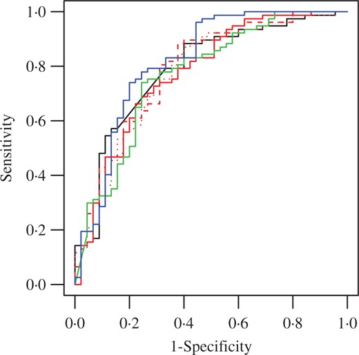
Receiver operating characteristic curves with the area under the curve, AUC, for leave-one-out crossvalidation of the EEG data by six different methods: lasso (black solid, AUC |$= 0.789$|⁠), functional principal component analysis using the leading eigenvectors that explain 80% (red solid, AUC |$= 0.775$|⁠), 90% (red dashes, AUC |$= 0.789$|⁠) or 95% (red dots, AUC |$= 0.777$|⁠) of variations, Gaussian process approach (green solid, AUC |$= 0.770$|⁠) and soft-thresholded Gaussian process approach (blue solid, AUC |$= 0.818$|⁠).

The differences between the models are further examined in the estimated |$\beta$| functions plotted in Fig. 4, where we ignore the spatial locations of the electrodes and plot them using their identification number. The lasso solution is nonzero for a single spatiotemporal location, while the functional principal component analysis and Gaussian process methods lead to nonsparse and thus uninterpretable |$\beta$| estimates. In contrast, the soft-thresholded Gaussian process-based estimate is near zero for the vast majority of locations, and isolates a subset of electrodes near time-point 86 as the most powerful predictors of alcoholism.

Fig. 4.

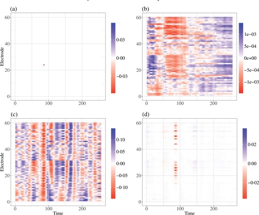
Estimated spatial-temporal effects of the EEG image predictors by four different methods: (a) lasso, (b) functional principal component analysis, (c) Gaussian process and (d) soft-thresholded Gaussian process. The Gaussian process and soft-thresholded Gaussian process estimates are posterior means.

Our analysis suggests that EEG measurements at time |$t=86$|⁠, which roughly corresponds to |$0.336$| fraction of second, are predictive of the alcoholism status. This observation is further confirmed by the plot of the posterior probability of nonzero |$\beta({s}_j, t)$| values in Fig. 5(a). This implies a delayed reaction to the stimulus, although this finding has to be confirmed with the investigators. To gain more insight into these findings, Figs. 5(b)–5(d) focus on a particular time and display the posterior mean and posterior probability of a nonzero signal across the electrode locations. They indicate that the right occipital/lateral region is the most predictive of alcoholism status.

Fig. 5.

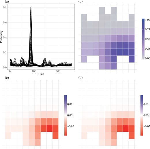
Summary of analysis of the EEG data by the soft-thresholded Gaussian process. Panel (a) plots the posterior probability of a nonzero |$\beta({s},t)$|⁠; each electrode is a line plotted over time |$t$|⁠. The remaining panels map either the posterior probability of a nonzero |$\beta({s},t)$| or the posterior mean of |$\beta({s},t)$| at individual time-points.

7. Discussion

The proposed method suggests future research directions. First, we aim to develop a more efficient posterior computation algorithm for analysis of voxel-level functional magnetic resonance imaging, fMRI, data, which typically contains 180 000 voxels for each subject. Any fast and scalable Gaussian processes approximation approach can be potentially applied to the soft-thresholded Gaussian process. For example, the nearest-neighbour Gaussian process approach proposed by Datta et al., (2016) can be applied to our model. In addition, it is of great interest to perform joint analysis of datasets involving multiple imaging modalities, such as fMRI, diffusion tensor imaging and structural MRI. It is very challenging to model the dependence between the multiple imaging modalities over space and to select the interactions between multiple-modality image predictors in scalar-on-image regression. The extension of the soft-thresholded Gaussian process might solve this problem. The basic idea is to introduce hierarchical latent Gaussian processes and different types of thresholding parameters for different modalities, leading to a hierarchical soft-thresholded Gaussian process as the prior model for the effects of interactions.

Acknowledgement

This research was supported partially by the U.S. National Institutes of Health and National Science Foundation. The authors would like to thank the editor, the associate editor and reviewers for suggestions that led to an improved manuscript.

Supplementary material

Supplementary material available at Biometrika online contains theoretical results and additional simulation study results.

Appendix

Conditions for theoretical results

 

Condition A1.

There exist |$M_0>0$|⁠, |$M_1>0$|⁠, |$N\geq 1$|⁠, and some |$\upsilon_0$| with |$d/(2\rho)<\upsilon_0<1$| and |$\rho = \lceil d/2\rceil$| such that for all |$n > N$|⁠, |$M_0 n^d \leq p_n \leq M_1 n^{2\rho \upsilon_0}$|⁠.

This condition implies that the number of image predictors |$p_n$| should be of polynomial order in the sample size. The lower bound indicates that |$p_n$| needs to be sufficiently large that the posterior distribution of the spatially varying coefficient function concentrates around the true value.

 

Condition A2.

The true spatially varying coefficient function in model (1) enjoys the piecewise smoothness, sparsity and continuity properties; in short, |$\beta_0 \in\Theta$|⁠.

The next two conditions summarize constraints on the spatial locations and the distribution of the image predictors.

 

Condition A3.

For the observed spatial locations |${S} = \{{s}_j\}_{j=1}^{p_n}$| in region |${\cal B}$|⁠, there exists a set of subregions |$\{{\cal B}_{j}\}_{j=1}^{p_n}$| satisfying the following conditions:

• A3.1 They form a partition of |${\cal B}$|⁠, i.e., |${\cal B} = \bigcup_{j=1}^{p_n} {\cal B}_{j}$| with |${\cal B}_{j}\cap {\cal B}_{j'} = \emptyset$|⁠.

• A3.2 For each |$j = 1,\ldots, p_n$|⁠, |${s}_j \in {\cal B}_j$| and |${V}({\cal B}_j) \leq \zeta({\cal B}_j) < \infty$|⁠, where V is the Lebesgue measure and |$\zeta({\cal B}) = \sup_{{t}, {t}'\in {\cal B}} \left(\max_{k} |t_{k} - t'_k|\right )^d, \ {\rm with} \ {t} = (t_1,\ldots, t_d)^{{\rm T}}, \ {\rm and} \ {t}' = (t'_1,\ldots, t'_d)^{{\rm T}}$|⁠.

• A3.3 There exists a constant |$0<K< {V}({\cal B})$| such that |$\max_{j} \zeta({\cal B}_j) < 1/(K p_n)$| as |$n\to\infty$|⁠.

When |${\cal B}$| is a hypercube in |$\mathbb{R}^d$|⁠, e.g., |${\cal B} = [0,1]^d$|⁠, there exists a set of |$\{{\cal B}_j\}_{j=1}^{p_n}$| that equally partitions |${\cal B}$|⁠. Then |${V}({\cal B}_j) = \zeta({\cal B}_j) = p^{-1}_{n}$|⁠.

 

Condition A4.

The covariate variables |$\{X_{i,1},\ldots, X_{i,p_n}\}_{i=1}^n$| are independent realizations of a stochastic process |$X({s})$| at spatial locations |${s}_1,\ldots, {s}_{p_n}$|⁠. And |$X({s})$| satisfies the following conditions:

• A4.1 |$E\{X({s})\} = 0$| for all |${s} \in {\cal B}$|⁠.

• A4.2 For all |$n >1$|⁠, let |${\Sigma}_n = (\sigma_{j,j'})_{1\leq j,j'\leq p_n}$| where |$\sigma_{j,j'}= E\{X({s}_j)X({s}_{j'})\}$|⁠. Let |$\rho_{\mathrm{min}}(A)$| and |$\rho_{\mathrm{max}}(A)$| be the smallest eigenvalue and the largest eigenvalue of a matrix |$A$|⁠, respectively. Then there exist |$c_{\rm min}$| and |$c_{\rm max}$| with |$0<c_{\rm min}\leq1$| and |$0 < c_{\rm max} < \infty$| such that for |$n>1$|⁠, |$\rho_{{\rm min}} \left({\Sigma}_n \right) > c_{\rm min}$| and |$\rho_{{\rm max}} \left({\Sigma}_n \right) < c_{\rm max}$|⁠.

• A4.3 For any |$\varepsilon>0$| and |$M<\infty$|⁠, there exists |$\delta > 0$| such that for any |$a_1,\ldots, a_{p_n} \in \mathbb R$| with |$|a_j|<M$| for all |$j$|⁠, if there exists |$N$| such that for all |$n > N$|⁠, |$p^{-1}\sum_{j=1}^{p_n}|a_j| > \varepsilon,$| then

  $$\Pi\left\{p_n^{-1/2}\left|\sum_{j=1}^{p_n} a_j X({s}_j)\right| > \delta \right\} > \delta\text{.}$$

Condition A4 includes assumptions on the mean of |$X({s})$| and on the range of eigenvalues of the covariance matrix |${\Sigma}_n$| for covariate variables. If the Gaussian process |$X({s})$| on |$[0,1]^d$| has zero mean and |${E}\{X({s}_j)X({s}_{j'})\} = \rho_0\exp(- p_{n}\|{s}_j-{s}_{j'}\|_1)$| with |$0<\rho_0<1$|⁠, for |$j\neq j'$| and |${E}\{X({s}_j)^2\} = 1$|⁠, where |$\{{s}_j\}_{j=1}^{p_n}$| are chosen as the centres of the equally spaced partitions of |${\cal B}$|⁠, then Condition A4|$\cdot$|2 holds. Furthermore, Condition A4|$\cdot$|3 also holds. Specifically, for any |$\varepsilon > 0$|⁠, taking |$\delta = c_{\rm min}^{1/2}\varepsilon\exp(-\varepsilon)$|⁠, for any |$a_1,\ldots, a_{p_n}$| let |$\xi = p_n^{-1/2}\sum_{j=1}^{p_n} a_j X({s}_j) \sim {N}(0, \kappa^2).$| By Condition A4|$\cdot$|2, |$\kappa^2 = p_n^{-1}\sum_{j,j'} a_j \sigma_{j,j'} a_{j'} \geq p_n^{-1} \sum_{j=1}^{p_n} a_j^2 \rho_{{\rm min}}({\Sigma}_n) > c_{{\rm min}}p_n^{-1} \sum_{j=1}^{p_n} a_j^2$|⁠.

There exists |$N$| such that for all |$n>N$|⁠, |$(p_n^{-1}\sum_{j=1}^{p_n} a_j^2)^{1/2} \geq p^{-1}_n \sum_{j=1}^{p_n} |a_j| > \varepsilon\text{.}$| Thus, |$\kappa^2>c_{{\rm min}}\varepsilon^2$|⁠. Furthermore, |$\Pi(|\xi| > \delta) =2\Phi(-\kappa^{-1}\delta) > 2\Phi (-c_{{\rm min}}^{-1/2}\varepsilon^{-1}\delta) = 2\Phi\{-\exp(-\varepsilon)\}>\varepsilon\exp(-\varepsilon)> \delta$|⁠.

To ensure the large-support property, we need the following condition on the kernel function of the Gaussian process. This condition has also been used previously by Ghosal & Roy (2006).

 

Condition A5.

For every fixed |${s} \in {\cal B}$|⁠, the covariance kernel |$\kappa({s},\cdot)$| has continuous partial derivatives up to order |$2\rho+2$|⁠. Suppose that |$\kappa({s},{t}) = \prod_{l=1}^d \kappa_l(s_l - t_l; \nu_l)$| for any |${s} = (s_1,\ldots, s_d)$| and |${t} = (t_1,\ldots,t_d)\in[0,1]^d$|⁠, where |$\kappa_l(\cdot; \nu_l)$| is a continuous, nowhere zero, symmetric density function on |${\mathbb R}$| with parameter |$\nu_l\in {\mathbb R}^{+}$| for |$l = 1,\ldots, d$|⁠.

Additional lemmas

 

Lemma A1.

The |$\varepsilon$|-covering number |$N(\varepsilon, \Theta_{n}, \|\cdot\|_{\infty})$| of |$\Theta_{n}$| in the supremum norm satisfies |$\log N(\varepsilon, \Theta_{n}, \|\cdot\|_{\infty})\leq Cp_n^{1/(2\rho)} \varepsilon^{-d/\rho}$|⁠. 

 

Lemma A2.

Suppose that Condition A3 holds for all |${s}_j$| for |$j = 1,\ldots, p_n$| and that |$K$| is the constant in Condition A3. Let |$\upsilon>0$| be a constant. For each integer |$n$|⁠, let |$\Lambda_n$| be a collection of continuous functions, where each function |$\gamma({s})$| is differentiable on a set |${\cal D}$| that is dense in |${\cal B}$| and |$\sup_{{s} \in {\cal D}} |D^{{\tau}}\gamma| \leq p_n^{\|{\tau}\|_1/2d}+\upsilon$| for |$\|{\tau}\|_1 \geq 0$|⁠. For each function |$\gamma\in \Lambda_n$| and |$\varepsilon > 0$|⁠, define |${\cal V}_{\varepsilon, \gamma} = \{{s}: |\gamma({s})| > \varepsilon \}$|⁠. For all |$n > N$| and |$\gamma \in \Lambda_n$|⁠, |$\sum_{j=1}^{p_n} |\gamma({s}_j)| \geq \lambda({\cal V}_{\varepsilon,\gamma})K \varepsilon p_n/2$|⁠. 

 

Lemma A3.

Suppose that Conditions A1 and A2 hold. For each |$\varepsilon>0$|⁠, there exist |$N$| and |$r>0$| such that for all |$n>N$| and for all |$\beta \in \Theta_n$| such that |$\|\beta -\beta_0\|_1 > \varepsilon$|⁠, we have |$\sum_{j=1}^{p_n} |\beta({s}_j) - \beta_0({s}_j)| > r p_n$|.

 

Lemma A4.

For any |$0<\varepsilon<1$| and |$0<r<\varepsilon^2$|⁠, let

$$A_n = \left[\sum_{i=1}^n p_n^{-1/2}\left|\sum_{j=1}^{p_n} X_{i,j}\{\beta({s}_j)-\beta_0({s}_j)\}\right| \geq n r\right]\!\text{.}$$

There exist |$N$| and |$D>0$| such that if for all |$n>N$| and for all |$\beta \in \Theta_n$|⁠, |$\Pi[ p_n^{-1/2}|\sum_{j=1}^{p_n} X({s}_j)\{\beta({s}_j)-\beta_0({s}_j)\}|>\varepsilon] > \varepsilon,$| then

\begin{eqnarray*} \Pi\left(A_n^C \right) \leq \varepsilon^2/r\exp(-D n), \quad \Pi\left(\bigcup_{m=1}^{\infty}\bigcap_{n=m}^\infty A_m\right) = 1\text{.} \end{eqnarray*}

 

Lemma A5.

Suppose that |${{\alpha}^{\rm v}_0} = (\alpha_{0,1},\ldots, \alpha_{0,q})^{{\rm T}}$| and |$\sigma^2_0$| are known. For the hypothesis testing problem |$H_0: \beta = \beta_0 \in \Theta$| versus |$H_1: \beta = \beta_1 \in \Theta$|⁠, the testing statistic is |$\Psi_n(\beta_0,\beta_1)= I\left\{\sum_{i=1}^n \delta_i (Y_i - \eta_{i,0})/\sigma_0 > 2 n^{\upsilon+1/2}\right\}$|⁠, where |$\eta_{i,m} = \sum_{k=1}^q \alpha_{0,k} W_{i,k} + p_n^{-1/2}\sum_{j=1}^{p_n} \beta_m({s}_j) X_{i,j}$| for |$m = 0,1$|⁠, |$\delta_i = 2I(\eta_{i,1} > \eta_{i,0})-1$| and |$\upsilon_0/2<\upsilon<1/2$|⁠. Then for any |$r>0$|⁠, there exist constants |$C_0$|⁠, |$C_1$|⁠, |$N$| and |$r_0>0$| such that for any |$\beta_0$| and |$\beta_1$| satisfying |$\sum_{j=1}^{p_n} |\beta_{1}({s}_j) - \beta_0({s}_j)| > r p_n$| for any |$n > N$|⁠, we have |${E}_{\beta_0}\{\Psi_n(\beta_0,\beta_1)\} \leq C_0\exp(-2 n^{2\upsilon})$|⁠, and for any |$\beta$| with |$\|\beta-\beta_1\|_{\infty} < r_0/(4c_{{\rm max}}^{1/2})$|⁠, we have |${E}_{\beta}\{1-\Psi_n(\beta_0,\beta_1)\} \leq C_0\exp(- C_1 n )$|⁠. 

Proof of Lemma 2

For any |$\lambda_0 > 0$|⁠, set |$\alpha({s}) = \beta_0({s}) + \lambda_0$| for |${s} \in \bar {\cal R}_1$| and |$\alpha({s}) = \beta_0({s}) - \lambda_0$| for |${s} \in \bar {\cal R}_{-1}$|⁠. Then by Condition A1, |$\alpha({s})$| is smooth over |$\bar {\cal R}_1 \cup \bar {\cal R}_{-1}$|⁠, i.e., |$\alpha({s})I({s} \in \bar {\cal R}_1 \cup \bar {\cal R}_{-1}) \in {\mathcal C}^{\rho}(\bar {\cal R}_1 \cup \bar {\cal R}_{-1})$|⁠. Next, we define |$\alpha({s})$| on another closed subset of |${\cal B}$|⁠. Since |${\cal B}$| is compact, |$\partial{\cal R}_k$| for |$k = -1,1$| is also compact. For any |$r > 0$| and each |${t} \in {\cal B}$|⁠, define an open ball |$B({t},r) = \{{s}: \|{t}-{s}\|_2<r\}$|⁠, where |$\|\cdot\|_2$| is the Euclidean norm. Note that |$\partial {\cal R}_k \subseteq \bigcup_{{t}\in \partial{\cal R}_k} B({t},r)$| for |$k = -1,1$|⁠. Since |$\partial{\cal R}_1 \cup\partial{\cal R}_{-1}$| is compact, there exists |${t}_l\in \partial {\cal R}_1 \cup \partial {\cal R}_{-1}$|⁠, for |$1\leq l\leq L$|⁠, such that |$\partial {\cal R}_{-1} \subseteq \bigcup_{l=1}^{L_0} B({t}_l,r)$| and |$\partial {\cal R}_1 \subseteq \bigcup_{l=L_0+1}^{L} B({t}_l,r)$|⁠.

Let |${\cal R}^*_0(r) = {\cal R}_0 - \bigcup_{l=1}^{L} B({t}_l,r)$|⁠; then |${\cal R}^*_0 \subseteq {\cal R}_0 - \partial {\cal R}_1 \cup \partial {\cal R}_{-1}$|⁠. Note that |${\cal R}_0 -\partial {\cal R}_1 \cup \partial {\cal R}_{-1}$| is a nonempty open set, |${\cal R}^*_0(r)$| is its closed subset and |${\cal R}^*_0(r)$| will increase as |$r$| decreases. There exists an |$r_0$|⁠, |$0<r_0<1$|⁠, such that |${\cal R}^*_0(r_0) \neq \emptyset$| and |$\{\bigcup_{l=1}^{L_0} B({t}_l,r_0)\}\cap \{\bigcup_{l=L_0}^{L} B({t}_l,r_0)\} = \emptyset$|⁠. The latter fact is due to |${\cal R}_1 \cap {\cal R}_{-1} = \emptyset$|⁠. Since |${\cal R}_{1}\cup{\cal R}_{-1}$| is bounded and |$\alpha\in{\mathcal C}^{\rho}({\cal R}_{1}\cup{\cal R}_{-1})$|⁠, we have |$M = \max_{0<\|{\tau}\|_1\leq \rho} \sup_{{t}\in {\cal R}_1\cup {\cal R}_{-1}}|D^{{\tau}}\alpha({t})| < \infty$|⁠. Take |$r = \min[\lambda_0/\{2M(\rho+1)^d+1\},r_0]$|⁠. Define |$\alpha({s}) = 0$| if |${s} \in {\cal R}^*_0(r)$|⁠. Then |$\alpha({s})$| is well defined on a closed set |${\cal R}^* = {\cal R}^*_0 \cup \bar {\cal R}_1 \cup \bar {\cal R}_{-1}$|⁠, where |${\cal R}^*_0 = {\cal R}^*_0(r)$|⁠.

Define a function |$\phi({s},{t}) = \sum_{\|{\tau}\|_1\leq \rho} D^{{\tau}}\alpha ({t})({s} - {t})^{{\tau}}/{\tau}!= \alpha({t}) + \sum_{0<\|{\tau}\|_1\leq \rho} D^{{\tau}}\alpha ({t})({s} - {t})^{{\tau}}/{\tau}!\text{.}$| When |${t} \in \partial {\cal R}_1 \cup \partial {\cal R}_{-1}$| and |${s} \in B({t},r_0)$|⁠, |$|\phi({s},{t})| \leq |\lambda_0| + \bigg|\sum_{0<\|{\tau}\|_1\leq \rho} D^{{\tau}}\alpha ({t})({s} - {t})^{{\tau}}/{\tau}!\bigg | \leq \lambda_0 + 2 M (\rho+1)^d r_0$|⁠. When |${t} \in \partial {\cal R}^*_0(r_0)$| and |$\|{s}-{t}\| < r_0$|⁠, |$|\phi({s},{t})|\leq 2M (\rho+1)^d r_0$|⁠.

Define |$\psi({t}) = \sum_{l=1}^L \psi({t},{t}_l)$|⁠, where |$\psi({t},{t}_l) = C_l\exp\{-1/(1-\|{t}-{t}_l\|_2/r)\}I(\|{t}-{t}_l\|_2<r)\text{.}$| We choose |$C_l$| for |$l = 1,\ldots, L$| such that |$\sum_{l=1}^{L}\int_{B({t}_l,r)}\psi({t},{t}_l)\, {\rm d} {t} = 1$| and |$\sum_{l=L_0+1}^{L}\int_{B({t}_l,r)}\psi({t},{t}_l)\,{\rm d} {t} < 1 - 2M(\rho+1)^d r/\lambda_0$|⁠. We construct |$\tilde \beta_0({s})$| by extending |$\alpha({s})$| from |${\cal R}^*$| to the whole domain |${\cal B}$|⁠. Let

\begin{eqnarray*} \tilde\beta_0({s}) = \left\{\begin{array}{ll} \int_{\partial {\cal R}^*} \phi({s}, {t}) \psi({t})\, {\rm d} {t} ,&{s} \in {\cal B} - {\cal R}^*,\\ \alpha({s}), & {s} \in {\cal R}^*\text{.} \end{array}\right. \end{eqnarray*}

Note that

\begin{eqnarray*} \bigg|\int_{\partial {\cal R}^*} \phi({s}, {t}) \psi({t}) \,{\rm d} {t}\bigg|&\leq&\sum_{l=1}^L \int_{\partial {\cal R}^* \cap B({t}_l,r)} \big| \phi({s}, {t}) \big| \psi({s},{t}) \,{\rm d} {t}\\ &\leq&\sum_{l=1}^L \left\{\int_{\partial {\cal R}^*_0 \cap B({t}_l,r)}\big| \phi({s}, {t})\big| \psi({s},{t}) \,{\rm d} {t} + \int_{\partial ({\cal R}_1\cup {\cal R}_{-1}) \cap B({t}_l,r)} \big|\phi({s}, {t}) \big|\psi({s},{t}) \,{\rm d} {t}\right\}\\ &< & 2M(\rho+1)^d r (1-w_{1}) + \{\lambda_0+2M(\rho+1)^d r\} w_{1} < \lambda_0, \end{eqnarray*}

where |$w_1 = \sum_{l=L_0+1}^{L}\int_{B({t}_l,r)}\psi({t},{t}_l)\,{\rm d} {t} < 1 - 2M(\rho+1)^d r/\lambda_0$|⁠.

Next, we show that |$\lim_{{s}\rightarrow {s}_0} D^{{\tau}} \tilde \beta_0({s}) = D^{{\tau}} \alpha({s}_0)$| for any |${s}_0 \in \partial {\cal R}^*$| and |${\tau}$| with |$\|{\tau}\|_1\leq \rho$|⁠.

For any |$\varepsilon$| with |$0<\varepsilon<1$|⁠, since |$D^{{\tau}}\alpha$| is continuous over |${\cal R}^*$|⁠, there exists |$\delta_1>0$| such that for all |${t}$| with |$\|{t} -{s}_0\|<\delta_1$|⁠, we have |$|D^{{\tau}}\alpha({t}) - D^{{\tau}}\alpha({s}_0)| < \varepsilon/2$|⁠. Take |$\delta < \min[\varepsilon/\{2 (\rho+1)^d M\}, r, \delta_1]$|⁠; then as long as |$\|{s}_0 - {s}\|< \delta$|⁠, we have

\begin{eqnarray*} |D^{{\tau}} \tilde \beta_0({s}) - D^{{\tau}} \tilde \alpha({s}_0)| &\leq & \int_{\partial {\cal R}^*}|D^{{\tau}}\alpha({t})-D^{{\tau}}\alpha({s}_0)|\psi({t})\,{\rm d} {t} + \hspace{-2mm} \sum_{\tiny \begin{array}{c}{\|{\tau}'\|_1 \geq \|{\tau}\|_1},\\ {\tau}'\neq {\tau}\end{array}} \int_{\partial {\cal R}^*}\frac{|D^{{\tau}'}\alpha({t})|}{{\tau}'!}|({s} - {t})^{{\tau}'}| \psi({t}) \,{\rm d} {t} \\ &<& \frac{\varepsilon}{2} + (\rho+1)^d M \delta < \varepsilon\text{.} \end{eqnarray*}

By Condition A2, we have |$\alpha({s}) = \lambda_0$| for |${s} \in \partial{\cal R}_1$|⁠, and |$\alpha({s}) = -\lambda_0$| for |${s}\in\partial{\cal R}_{-1}$|⁠.