Adaptive multigroup confidence intervals with constant coverage

SUMMARY

Commonly used interval procedures for multigroup data attain their nominal coverage rates across a population of groups on average, but their actual coverage rate for a given group will be above or below the nominal rate, depending on the group mean. While correct coverage for a given group can be achieved with a standard |$t$|-interval, this approach is not adaptive to the available information about the distribution of group-specific means. In this article we construct confidence intervals that have a constant frequentist coverage rate and that make use of information about across-group heterogeneity, resulting in constant-coverage intervals that are narrower than standard |$t$|-intervals on average across groups. Such intervals are constructed by inverting biased Bayes-optimal tests for the mean of each group, where the prior distribution for a given group is estimated with data from the other groups.

1. Introduction

A commonly used experimental design is the one-way layout, in which a random sample |$Y_{1,j},\ldots, Y_{n_j,j}$| is obtained from each of several related groups |$j\in \{1,\ldots, p\}$|⁠. The standard normal-theory model for data from such a design is that |$Y_{i,j} \sim N(\theta_j,\sigma^2)$| independently within and across groups. Inference for the |$\theta_j$| typically proceeds in one of two ways. The classical approach is to use the sample mean |$\bar y_j$| as an estimator of |$\theta_j$|⁠, and to use the standard |$t$|-interval as a confidence interval. Such an approach essentially makes inference for each |$\theta_j$| using only data from group |$j$|⁠, although a pooled estimate of |$\sigma^2$| is often used. The estimator of each |$\theta_j$| is unbiased, and the confidence interval for each |$\theta_j$| has the desired coverage rate.

An alternative approach is to use data from all of the groups to infer each individual |$\theta_j$|⁠, typically by invoking a hierarchical model to describe the heterogeneity across the groups. The one-way random-effects model posits that |$\theta_1,\ldots, \theta_p$| are a random sample from a normal population with some mean |$\mu$| and variance |$\tau^2$|⁠. In this case, shrinkage estimators of the form

\[ \hat \theta_j = \frac{ \hat \mu/\hat \tau^2 + \bar y_j n_j/\hat \sigma^2} { 1/\hat \tau^2 + n_j/\hat \sigma^2 } \]

are often used, where |$(\hat \mu, \hat \tau^2, \hat \sigma^2)$| are estimated using data from all of the groups. The estimator |$\hat\theta_j$| has a lower variance than |$\bar y_j$| but is biased. A confidence interval centred around |$\hat\theta_j$| is often derived from the following hierarchical model. Letting

\[ \tilde\theta_j = \frac{ \mu/ \tau^2 + \bar y_j n_j/ \sigma^2} { 1/\tau^2 + n_j/ \sigma^2 }, \]

we have |$E\{(\tilde \theta_j - \theta_j)^2\} = (1/\tau^2 + n_j/\sigma^2)^{-1}$|⁠, where the expectation integrates over both the normal model for the observed data and that representing heterogeneity across the groups. This expectation is also the conditional variance of |$\theta_j$| given data from group |$j$|⁠, which suggests an empirical Bayes posterior interval for |$\theta_j$| of the form |$ \hat \theta_j \pm t_{1-\alpha/2 } / (1/\hat \tau^2 +n_j/\hat \sigma^2 )^{1/2}$|⁠, where |$t_\gamma$| denotes the |$\gamma$|-quantile of the appropriate |$t$| distribution. Compared with the classical |$t$|-interval |$\bar y_j \pm t_{1-\alpha/2} \times (\hat\sigma^2/n_j)^{1/2}$|⁠, this interval is narrower by a factor of |$\{ \hat\tau^2 /(\hat \tau^2 + \hat\sigma^2/n_j) \}^{1/2}$|⁠, but its coverage rate is not |$1-\alpha$| for all groups. While the rate tends to be near the nominal level on average across all groups, the rate for a specific group |$j$| will depend on the value of |$\theta_j$|⁠. Specifically, the coverage rate will be too low for those |$\theta_j$| far from the overall average |$\theta$|-value, and too high for the |$\theta_j$| that are close to this average (Snijders & Bosker, 2012, § 4.8). Other types of empirical Bayes posterior intervals have been developed by Morris (1983), Laird & Louis (1987), He (1992) and Hwang et al. (2009). Like the interval obtained from the hierarchical normal model, these intervals are narrower than the standard |$t$|-interval but fail to have the target coverage rate for each group.

In the related literature on confidence region construction for a vector of normal means, several authors have pursued procedures that dominate those based on uniformly most powerful test inversion (Berger, 1980; Casella & Hwang, 1986). In particular, Tseng & Brown (1997) obtained a modified empirical Bayes confidence region that has exact frequentist coverage but is also uniformly shorter than that obtained by the usual procedure. In this article we develop a confidence interval procedure that has the desired coverage rate for every group, but which also adapts to the heterogeneity across groups, thereby achieving shorter confidence intervals than the classical approach on average across groups. More precisely, our goal is to obtain a multigroup confidence interval procedure |$\{ C^1(Y),\ldots, C^p(Y)\}$|⁠, based on data |$Y$| from all of the groups, which attains the target frequentist coverage rate for each group and all values of |$\theta=(\theta_1,\ldots,\theta_p)$|⁠, so that

\begin{equation} {\rm pr}\{ \theta_j \in C^j(Y) \mid \theta\} = 1-\alpha \quad (\theta \in \mathbb R^p;\: j\in \{1,\ldots, p\}), \end{equation}

(1)

and is also more efficient than the standard |$t$|-interval on average across groups, so that

\begin{equation} {E}{ | C^j(Y)| } < 2 t_{1-\alpha/2} \times (\hat \sigma^2/n_j)^{1/2}, \end{equation}

(2)

where |$|C|$| denotes the width of an interval |$C$| and the expectation is with respect to an unknown distribution describing the across-group heterogeneity of the |$\theta_j$|⁠. Our procedures satisfy the constant-coverage property (1) exactly. Property (2) will hold approximately, depending on what the across-group distribution is and how well it is estimated.

The intuition behind our procedure is as follows: while the standard |$t$|-interval for a single group is uniformly most accurate among unbiased interval procedures, it is not uniformly most accurate among all procedures. We define classes of biased hypothesis tests for a normal mean, inversion of which generates |$1-\alpha$| frequentist |$t$|-intervals that are more accurate than the standard |$t$|-interval for some values of the parameter space, but are less accurate elsewhere. The class of tests can be chosen to minimize an expected width with respect to a prior distribution for the population mean, yielding a confidence interval procedure that is Bayes-optimal among all procedures that have |$1-\alpha$| frequentist coverage. Such a procedure may be viewed as frequentist but assisted by Bayes. In a multigroup setting, the prior for a group mean is replaced by a model for across-group heterogeneity. The parameters in this model can be estimated using data from all of the groups, yielding an empirical Bayes-optimal confidence interval procedure that maintains a coverage rate which is constant as a function of the group means.

Several authors have studied constant-coverage interval procedures in the single-group case that differ from the standard procedure. Such alternative procedures generally make use of some sort of prior knowledge about the population mean. In particular, our work builds upon that of Pratt (1963), who studied the Bayes-optimal |$z$|-interval for the case where |$\sigma^2$| is known. Other related work includes that of Puza & O’Neill (2006), Farchione & Kabaila (2008) and Kabaila & Tissera (2014), who developed procedures which make use of prior knowledge that the mean is near a prespecified parameter value, such as zero. The procedures developed in the latter two articles have shorter expected widths near this special value, but revert to standard procedures when the data are far from this point. The former work was extended in Puza & O’Neill (2009) and Puza & Yang (2011) to provide confidence intervals for the means of Poisson and binomial populations in cases where there are known constraints on the parameter. Related to this, Evans et al. (2005) obtained minimax interval procedures for cases where prior knowledge takes the form of bounds on the parameter values.

2. Bayes-optimal frequentist intervals

2.1. Pratt’s |$z$|-interval

Consider a model for a random variable |$Y$| that is indexed by a single unknown scalar parameter |$\theta\in \mathbb R$|⁠. A |$1-\alpha$| confidence region procedure for |$\theta$| based on |$Y$| is a set-valued function |$C(y)$| such that |${\rm pr}\{ \theta \in C(Y) \mid \theta\} =1-\alpha$| for all |$\theta\in \mathbb R$|⁠. Such a procedure can be constructed by inversion of a collection of hypothesis tests. For each |$\theta\in \mathbb R$|⁠, let |$A(\theta)$| be the acceptance region of a level-|$\alpha$| test of |$H_\theta: Y \sim P_\theta$| versus |$K_\theta: Y\sim P_{\theta'}, \,\theta'=\hspace{-8pt}|\,\,\theta$|⁠. Then |$C(y) = \{ \theta: y \in A(\theta)\}$| is a |$1-\alpha$| confidence procedure. We take the risk |$R(\theta,C)$| of a |$1-\alpha$| confidence procedure to be its expected Lebesgue measure,

\[ R(\theta,C) = \int \!\!\int 1\{ y \in A(\theta')\} \,{\rm d}\theta' \, P_\theta({\rm d} y)\text{.} \]

For our current model of interest, |$Y\sim N(\theta,\sigma^2)$| with |$\sigma^2$| known, there does not exist a procedure that uniformly minimizes this risk over all values of |$\theta$|⁠. However, there exist optimal procedures within certain subclasses of procedures. For example, the standard |$z$|-interval, given by |$C_z(y) =( y+\sigma z_{\alpha/2} ,\, y+\sigma z_{1-\alpha/2})$|⁠, minimizes the risk among all unbiased procedures derived by inversion of unbiased tests of |$H_\theta$| versus |$K_\theta$|⁠, and so is the uniformly most accurate unbiased procedure.

That the interval is unbiased means |${\rm pr}\{ \theta' \in C_{z}(Y) \mid\theta\} \leqslant 1-\alpha$| for all |$\theta$| and |$\theta'$|⁠, and that it is uniformly most accurate means |$R(\theta,C_{z}) = 2\sigma z_{1-\alpha/2}\leqslant R(\theta,\tilde C)$| for any other unbiased procedure |$\tilde C$| and every |$\theta$|⁠. But while |$C_{z}$| is best among unbiased procedures, the lack of a uniformly most powerful test of |$H_\theta$| versus |$K_\theta$| means there will be procedures corresponding to collections of biased level-|$\alpha$| tests that have lower risks than |$C_{z}$| for some values of |$\theta$|⁠. This suggests that if we have prior information that |$\theta$| is likely to be near some value |$\mu$|⁠, we may be willing to incur larger risks for |$\theta$|-values far from |$\mu$| in exchange for small risks near |$\mu$|⁠. With this in mind, we consider the Bayes risk |$R(\pi, C) = \int R(\theta,C)\, \pi({\rm d}\theta)$|⁠, where |$\pi$| is a prior distribution that describes how close |$\theta$| is likely to be to |$\mu$|⁠. This Bayes risk may be related to the marginal probability of accepting |$H_\theta$| as follows:

\begin{align*} R(\pi,C) = \int R(\theta,C)\, \pi(\text{d}\theta) &= \int\!\!\int\!\!\int 1\{ y\in A(\theta')\} \, {\rm d} \theta' P_\theta({\rm d} y) \, \pi({\rm d}\theta) \\ &=\int\!\!\int\!\!\int 1\{ y\in A(\theta')\} P_\theta({\rm d} y) \,\pi({\rm d}\theta) \, {\rm d}\theta' \\ &= \int {\rm pr}\{ Y\in A(\theta') \} \, {\rm d}\theta'\text{.} \end{align*}

The Bayes-optimal |$1-\alpha$| procedure is obtained by choosing |$A(\theta)$| to minimize |${\rm pr}\{Y\in A(\theta)\}$| for each |$\theta\in\mathbb R$| or, equivalently, to maximize the probability of |$H_\theta$| being rejected under the marginal distribution |$P_\pi$| for |$Y$| that is induced by |$\pi$|⁠. This means that the optimal |$A(\theta)$| is the acceptance region of the most powerful test of the simple hypothesis |$H_\theta: Y \sim P_\theta$| versus the simple hypothesis |$K_\pi: Y \sim P_\pi$|⁠. The confidence region obtained by inversion of this collection of acceptance regions is Bayes-optimal among all procedures having |$1-\alpha$| frequentist coverage.

Using this logic, Pratt (1963) derived and studied the Bayes-optimal frequentist procedure for the model |$Y\sim N(\theta,\sigma^2)$| with |$\sigma^2$| known and prior distribution |$\theta\sim N(\mu,\tau^2)$|⁠. Under this distribution for |$\theta$|⁠, the marginal distribution of |$Y$| is |$N(\mu,\tau^2+\sigma^2)$|⁠. The Bayes-optimal procedure is therefore obtained by inverting acceptance regions |$A(\theta)$| of the most powerful tests of |$H_\theta: Y\sim N(\theta,\sigma^2)$| versus |$K_\pi: Y\sim N(\mu,\tau^2+\sigma^2)$| for each |$\theta$|⁠. This optimal procedure is an interval, the endpoints of which may be obtained by solving two nonlinear equations.

The procedure used to obtain Pratt’s |$z$|-interval and the form used by Pratt are not immediately extendable to the more realistic situation in which |$Y_1,\ldots, Y_n$| is a random sample from a |$N(\theta, \sigma^2)$| population where both |$\theta$| and |$\sigma^2$| are unknown. The primary reason is that in this case the Bayes-optimal acceptance region depends on the unknown value of |$\sigma^2$| or, to put it another way, the null hypothesis |$H_\theta$| is composite. However, the situation is not too difficult to remedy. Below we re-express Pratt’s |$z$|-interval in terms of a function that controls where the Type I error is spent. We then define a class of |$t$|-intervals based on such functions, from which we obtain the Bayes-optimal |$t$|-interval for the case where |$\sigma^2$| is unknown.

2.2. The Bayes-optimal |$w$|-function

For the model |$\{Y\sim N(\theta,\sigma^2), \, \theta\in \mathbb R\}$|⁠, we may limit consideration of confidence procedures to those obtained by inverting collections of two-sided tests.

 

Proposition 1.

Suppose that the distribution of |$Y$| belongs to a one-parameter exponential family with parameter |$\theta \in \mathbb{R}$|⁠. For any confidence region procedure |$\tilde C$| there exists a procedure |$C$|⁠, obtained by inverting a collection of two-sided tests, that has the same coverage as |$\tilde C$| and a risk less than or equal to that of |$\tilde C$|⁠.

This proposition follows from Ferguson (1967, § 5.3), which says that for any level-|$\alpha$| test of a point null hypothesis for a one-parameter exponential family, there exists a two-sided test of equal or greater power.

For the normal model of interest, an interval |$A(\theta)=(\theta-\sigma u ,\,\theta-\sigma l)$| will be the acceptance region of a two-sided level-|$\alpha$| test if and only if |$u$| and |$l$| satisfy |$\Phi(u) - \Phi(l) = 1-\alpha$| or, equivalently, |$u=z_{1-\alpha w}$| and |$l = z_{\alpha (1-w)}$| for some value of |$w\in [0,1]$|⁠, where |$\Phi$| is the standard normal cumulative distribution function and |$z_{\gamma} = \Phi^{-1}(\gamma)$|⁠. The value of |$w$|⁠, and hence the values of |$l$| and |$u$|⁠, can vary with |$\theta$| and still yield a |$1-\alpha$| confidence region. Let |$w:\mathbb R \rightarrow [0,1]$| and define |$A_w(\theta) = (\theta - \sigma z_{1-\alpha w(\theta)}, \,\theta-\sigma z_{\alpha\{1-w(\theta)\}} )$|⁠. Then for each |$\theta$|⁠, |$\:A_w(\theta)$| is the acceptance region of a level-|$\alpha$| test of |$H_\theta$| versus |$K_\theta$|⁠. Inversion of |$A_w(\theta)$| yields a |$1-\alpha$| procedure

\begin{equation} C_w(y) = \{ \theta : y+\sigma z_{\alpha \{1-w(\theta)\}} < \theta < y+\sigma z_{1-\alpha w(\theta)} \}\text{.} \end{equation}

(3)

That this procedure has |$1-\alpha$| constant coverage follows from the fact that it is obtained from the inversion of a class of level-|$\alpha$| tests. Alternatively, the constant-coverage property of (3) can be shown directly, as was done in Puza & O’Neill (2006). This calculation is provided for clarity here.

 

Proposition 2.

If |$w:\mathbb R \rightarrow [0,1]$|⁠, then |$C_w$| as given by (3) has constant coverage, that is, |${\rm pr}\{ \theta \in C_w(Y) \mid \theta,\sigma^2 \} =1-\alpha$| for every |$\theta\in\mathbb R$| and |$\sigma^2>0$|⁠.

 

Proof.

The coverage probability is |$ {\rm pr}\{ -z_{1-\alpha w(\theta) } < (Y-\theta)/\sigma < -z_{\alpha\{1- w(\theta)\} } \mid \theta,\sigma^2 \} \text{.} $| Since |$(Y-\theta)/\sigma$| is standard normal, this reduces to |$ [ 1 - \alpha\{1-w(\theta)\} ] - \alpha w(\theta) = 1-\alpha $|⁠. □

Every such |$w$|-function corresponds to a confidence procedure that has exact |$1-\alpha$| constant coverage; |$w$| can even be stochastic if it is independent of |$Y$|⁠.

The usual |$z$|-interval is |$ C_{1/2}(y) = \{ \theta : y+\sigma z_{\alpha /2 } < \theta < y+\sigma z_{1-\alpha/2} \}$|⁠, corresponding to a constant |$w$|-function of |$w(\theta)=1/2$|⁠. For the prior distribution |$\theta\sim N(\mu,\tau^2)$| considered by Pratt, the optimal |$w$|-function depends on |$\psi=(\mu,\tau^2,\sigma^2)$| and is given as follows.

 

Proposition 3.

Let |$Y\sim N(\theta,\sigma^2)$| with |$\theta\sim N(\mu,\tau^2)$|⁠, and let |$w:\mathbb R \rightarrow [0,1]$|⁠. Then |$R(\psi , C_{w_\psi} ) \leqslant R(\psi ,C_w)$| where |$ w_\psi(\theta) = g^{-1} \{ 2\sigma(\theta-\mu)/\tau^2 \} $| with |$g(w) = \Phi^{-1}(\alpha w) - \Phi^{-1}\{\alpha(1-w) \}$|⁠. The function |$w_\psi(\theta)$| is a continuous strictly increasing function of |$\theta$|⁠.

As stated in Pratt (1963) but not proven, |$C_{w_{\psi}}(y)$| is actually an interval for each |$y\in \mathbb R$|⁠, and so |$C_{w_\psi}$| is a confidence interval procedure. In fact, a confidence procedure |$C_w$| will be an interval procedure as long as the |$w$|-function is continuous and nondecreasing.

 

Proposition 4.

Let |$w: \mathbb R \rightarrow [0,1]$| be a continuous nondecreasing function. Then the set |$C_w(y) = \{ \theta : y+\sigma z_{\alpha \{1-w(\theta)\}} < \theta < y+\sigma z_{1-\alpha w(\theta)} \} $| is the interval |$(\theta^{\rm L},\theta^{\rm U})$|⁠, where to |$\theta^{\rm L} = y+ \sigma z_{\alpha\{1-w(\theta^{\rm L})\}}$| and |$\theta^{\rm U} = y+ \sigma z_{1-\alpha w(\theta^{\rm U})}$|⁠.

Pratt’s |$z$|-interval can be expressed as |$C_{w_\psi} = (\theta^{\rm L}, \theta^{\rm U})$| where

\begin{align*} \theta^{\rm U} &=\frac{y+\sigma \Phi^{-1}\big\{1-\alpha+\Phi\bigl(\tfrac{y-\theta^{\rm U}}{\sigma}\bigr)\big\}} {1+ 2\sigma^2/\tau^2 } + \mu \frac{2\sigma^2/\tau^2} { 1+ 2\sigma^2/\tau^2 }, \\ \theta^{\rm L} &=\frac{y+\sigma\Phi^{-1}\big\{\alpha - \Phi\bigl(\tfrac{\theta^{\rm L}-y}{\sigma}\bigr)\big\}} {1+ 2\sigma^2/\tau^2 } + \mu \frac{2\sigma^2/\tau^2} { 1+ 2\sigma^2/\tau^2}\text{.} \end{align*}

Solutions to these equations can be found with a zero-finding algorithm and by noting that |$\theta^{\rm L} < y+ \sigma z_{\alpha}$| and |$y+\sigma z_{1-\alpha} < \theta^{\rm U}$|⁠.

Some aspects of Pratt’s |$z$|-interval are displayed in Fig. 1. Panel (a) plots the |$w$|-functions corresponding to the Bayes-optimal 95% confidence interval procedures for |$\sigma^2=1$|⁠, |$\mu=0$| and |$\tau^2 \in \{1/4,1,4\}$|⁠. At varying rates depending on |$\tau^2$|⁠, the |$w$|-functions approach 0 and 1 as |$\theta$| moves towards |$-\infty$| and |$\infty$|⁠, respectively. The level-|$\alpha$| tests corresponding to these |$w$|-functions are spending more of their Type I error on |$y$|-values that are likely under the |$N(\mu,\sigma^2+\tau^2)$| prior predictive distribution of |$Y$|⁠. This makes the intervals narrower than the usual interval when |$y$| is near |$\mu$|⁠, and wider when |$y$| is far from |$\mu$|⁠, as shown in Fig. 1(b). In particular, at |$y=\mu$|⁠, the 95% interval with |$\tau^2=1/4$| has a width of 3|$\cdot$|29, which is about 84% that of the standard interval. If |$\tau^2=0$|⁠, then |$w(\theta)=1$| if |$\theta>\mu$| and |$w(\theta)=0$| if |$\theta< \mu$|⁠. The value of |$w(\mu)$| when |$\tau^2=0$| does not affect the width of the confidence interval, but can affect whether or not |$\mu$| is included in the interval as an endpoint. We suggest taking |$w(\mu)$| to be |$1/2$| when |$\tau^2=0$|⁠, as it is in the case of |$\tau^2>0$|⁠.

Fig. 1.

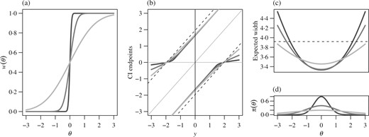
Descriptions of Pratt’s 95% |$z$|-interval procedure: (a) Bayes-optimal |$w$|-functions for |$\tau^2=1/4,1,4$| in decreasingly dark lines; (b) the corresponding confidence interval, CI, procedures, with the standard procedure represented by dashed lines; (c) the expected widths of the 95% |$z$|-intervals for the three values of |$\tau^2$|⁠, along with (d) the corresponding prior densities. Dashed lines in (b)–(d) correspond to the usual |$z$|-interval.

Average performance across |$y$|-values, or the expected confidence interval width, is displayed in Fig. 1(c). The expected widths of Pratt’s |$z$|-intervals are smaller than those of the usual intervals for values of |$\theta$| near |$\mu$|⁠, 15% less for |$\theta=\mu$| and |$\tau^2=1/4$|⁠, but can be much greater for |$\theta$|-values far away from |$\mu$|⁠, particularly for small values of |$\tau^2$|⁠. Relative to small values of |$\tau^2$|⁠, the larger value |$\tau^2=4$| enjoys better performance than the standard interval over a wider range of |$\theta$|-values, but the improvement is not as large near |$\mu$|⁠. Additional calculations show that the performance of Pratt’s |$z$|-interval near |$\mu$| improves as |$\alpha$| increases, as compared to the usual interval. For example, with |$\tau^2=1/4$| and |$\alpha=0{\cdot}50$|⁠, the width of Pratt’s interval at |$y=\mu$| is about 25% that of the usual interval, and its risk at |$\theta=\mu$| is 60% that of the usual interval.

2.3. Bayes-optimal |$t$|-intervals

Adoption of Pratt’s |$z$|-interval has been limited, possibly due to two issues: first, in most applications the population variance is unknown; and second, the prior distribution for |$\theta$| must be specified. We now address the first issue by developing a Bayes-optimal |$t$|-interval. Suppose we have a random sample |$Y_1,\ldots, Y_n$| from a |$N(\theta,\sigma^2)$| population, with sufficient statistics |$(\bar Y, S^2)$|⁠, the sample average and unbiased sample variance. The standard |$t$|-interval is given by |$\{ \theta: \bar y + n^{-1/2} s t_{\alpha/2} < \theta < \bar y + n^{-1/2} s t_{1-\alpha/2} \}$|⁠. This interval is symmetric about |$\bar y$|⁠, with the same tail-area probability of |$\alpha/2$| defining the lower and upper endpoints. The development of the |$w$|-function described in the previous subsection suggests viewing the standard |$t$|-interval as belonging to the larger class of confidence procedures given by

\begin{align} C_w(\bar y,s^2) &= \{ \theta: \bar y + n^{-1/2}st_{\alpha\{1-w(\theta)\}} < \theta < \bar y + n^{-1/2}s t_{1-\alpha w(\theta)} \}, \end{align}

(4)

for some |$w:\mathbb R \rightarrow [0,1]$|⁠. By the same logic as for the class of |$z$|-intervals of the form (3), any procedure of the form (4) has |$1-\alpha$| constant coverage.

 

Proposition 5.

If |$w:\mathbb R \rightarrow [0,1]$|⁠, then |$C_w$| as defined by (4) has constant coverage, that is, |${\rm pr}\{ \theta \in C_w(\bar Y,S^2) \mid \theta,\sigma^2 \} =1-\alpha$| for every |$\theta\in\mathbb R$| and |$\sigma^2>0$|⁠.

Additionally, |$C_w$| is an interval as long as |$w$| is a continuous nondecreasing function.

 

Proposition 6.

Let |$w: \mathbb R \rightarrow [0,1]$| be a continuous nondecreasing function. Then the set |$C_w(\bar y,s^2) = \{ \theta: \bar y + n^{-1/2}s t_{\alpha\{1-w(\theta)\}} < \theta < \bar y + n^{-1/2}s t_{1-\alpha w(\theta)} \}$| is the interval |$(\theta^{\rm L},\theta^{\rm U})$|⁠, where |$\theta^{\rm L} = \bar y+ n^{-1/2} s t_{\alpha\{1-w(\theta^{\rm L})\}}$| and |$\theta^{\rm U} = \bar y+ n^{-1/2} s t_{1-\alpha w(\theta^{\rm U})}$|⁠.

For a given |$w$|-function, the endpoints of the interval can be re-expressed as

\begin{equation} F \!\left (\frac{ \bar y - \theta^{\rm U} }{n^{-1/2}s}\right) = \alpha w(\theta^{\rm U}) , \quad F\!\left (\frac{\bar y-\theta^{\rm L} }{n^{-1/2}s}\right) = 1- \alpha\{1- w(\theta^{\rm L})\}, \end{equation}

(5)

where |$F$| is the |$t_{n-1}$| cumulative distribution function.

Using the logic at the beginning of § 2, the Bayes risk of a confidence procedure for a prior distribution |$\pi$| on |$\theta$| and |$\sigma^2$| is |$R(\pi,C) = \int {\rm pr}\{ (\bar Y , S^2) \in A(\theta')\} \, {\rm d}\theta'$|⁠, where |${\rm pr}\{ ( \bar Y , S^2) \in A(\theta')\}$| is the marginal, or prior predictive, probability of |$(\bar Y, S^2)$| being in the acceptance region |$A(\theta')$| under the prior distribution |$\pi$|⁠. Given a prior |$\pi$| that corresponds to a continuous nondecreasing |$w$|-function, the Bayes-optimal interval can be obtained by using an iterative algorithm to solve the equations in (5). However, this requires computation of the |$w$|-function, which for each |$\theta$| is the minimizer in |$w$| of |${\rm pr}\{ (\bar Y , S^2) \in A_w(\theta) \}$|⁠, where

\begin{equation*} A_w(\theta) = \left \{ (\bar y, s^2): t_{\alpha w} < \frac{\bar y - \theta }{n^{-1/2}s} < t_{1-\alpha(1-w) } \right \}\!\!\text{.} \end{equation*}

Obtaining the optimal |$w$|-function will generally involve numerical integration. Consider a |$N(\mu,\tau^2)$| prior on |$\theta$|⁠, so conditionally on |$\sigma^2$| we have |$\bar Y \sim N( \mu , \sigma^2/n + \tau^2)$| and |$(n-1)S^2/\sigma^2 \sim \chi^2_{n-1}$|⁠. From this we can show that |$c (\bar Y -\theta)/(n^{-1/2}S) $| has a noncentral |$t_{n-1}$| distribution with noncentrality parameter |$\lambda= c n^{1/2}(\mu -\theta)/\sigma $|⁠, where |$c = \{ (\sigma^2/n)/({\sigma^2/n+\tau^2})\}^{1/2}$|⁠. Therefore, the probability of the event |$\{ (\bar Y , S^2) \in A(\theta)\}$|⁠, conditional on |$\sigma^2$|⁠, can be written as

\[ {\rm pr}\{ ( \bar Y, S^2 ) \in A(\theta)\mid\sigma^2\} = F_\lambda( ct_{1-\alpha(1-w)}) - F_\lambda( ct_{\alpha w }), \]

where |$F_\lambda$| is the cumulative distribution function of the noncentral |$t_{n-1}$| distribution with parameter |$\lambda$|⁠. The Bayes-optimal |$w$|-function is therefore given by

\begin{equation} w_{\pi}(\theta) = \mathop{\arg\min}_w \int \big\{ F_\lambda( ct_{1-\alpha(1-w)}) - F_\lambda( ct_{\alpha w }) \big\} p_\pi(\sigma^2) \, {\rm d}\sigma^2, \end{equation}

(6)

where |$p_\pi(\sigma^2)$| is the prior density over |$\sigma^2$|⁠.

We provide R code in the Supplementary Material for obtaining |$w_{\pi}(\theta)$| and the corresponding Bayes-optimal |$t$|-interval |$C_{\pi}( \bar y,s^2)$| for |$\theta$| and |$\sigma^2$| being a priori independently distributed as normal and inverse-gamma random variables. For comparison with Pratt’s |$z$|-interval, one can consider the case where |$n=10$|⁠, |$1/\sigma^2 \sim {\rm Ga}(1,10)$| and |$\theta\sim N(0,\tau^2)$| for |$\tau^2 \in \{1/4,1,4\}$|⁠. This makes the prior median of |$\sigma^2$| near 10 and the variance of |$\bar Y$| near 1, and so the variance of |$\bar Y$| here is comparable to the variance of |$Y$| in § 2.1. Plots analogous to the panels of Fig. 1 are very similar to those in the |$z$|-interval case. In particular, the |$t$|-intervals resemble the corresponding |$z$|-intervals, but are slightly wider due to the use of |$t$|-quantiles instead of |$z$|-quantiles.

3. Empirical Bayes-optimal frequentist intervals for multigroup data

3.1. Constant-coverage empirical Bayes intervals via data splitting

A potential obstacle to the adoption of Bayes-optimal frequentist confidence intervals is the aversion that many researchers have to specifying a distribution over |$\theta$|⁠. However, in multigroup data settings, probabilistic information about the mean of one group may be obtained from data on the other groups. This information can be used to choose a |$w$|-function with which to construct a confidence interval. For example, suppose we have a class of |$w$|-functions |$\{ w_\psi : \psi\in \Psi\}$| we wish to select from, such that |$w_\psi:\mathbb R\rightarrow [0,1]$| for each |$\psi\in \Psi$|⁠. Let |$Y_1,\ldots, Y_n$| be a random sample from a |$N(\theta,\sigma^2)$| population, and let |$\hat\psi$| be a random variable, independent of |$Y_1,\ldots, Y_n$| and taking values in |$\Psi$|⁠. Then the random interval procedure given by |$C_{w_{\hat\psi}}$| will still have constant |$1-\alpha$| coverage, even though the |$w$|-function is stochastic.

 

Proposition 7.

If |$\bar Y \sim N(\theta, \sigma^2/n)$| and |$ (n-1) S^2/\sigma^2 \sim \chi^2_{n-1}$|⁠, and if |$\bar Y$|⁠, |$S^2$| and |$\hat\psi$| are independent, then |${\rm pr}\{ \theta\in C_{w_{\hat\psi}}(\bar Y, S^2) \mid \theta,\sigma^2\}=1-\alpha$|⁠.

 

Proof.

Because |$\hat\psi$| is independent of |$(\bar Y, S^2)$|⁠, the coverage of |$C_{w_{\hat\psi}}$| conditional on |$\hat\psi= \psi$| is the same as that of |$C_{w_{\psi}}$|⁠, which has coverage |$1-\alpha$| for all |$\psi\in \Psi$| by Proposition 5. □

In the multigroup setting, an adaptive procedure |$C_{w_{\hat\psi}}$| for the mean |$\theta_j$| of one group may be constructed by estimating the parameters |$\hat\psi$| in the hierarchical normal model using data from the other groups. Such an interval will have exact |$1-\alpha$| coverage for every value of |$\theta_j$| by Proposition 7, but will also have a shorter expected width for values of |$\theta_j$| that are deemed likely by |$\hat\psi$|⁠.

3.2. Asymptotically optimal procedure for homoscedastic groups

Consider the case of |$p$| normal populations with means |$\theta_1,\ldots, \theta_p$| and with common variance |$\sigma^2$| and sample size |$n$|⁠, so that |$Y_{i,j} \sim N(\theta_j,\sigma^2)$| independently within and across groups. We use a common sample size solely to simplify notation. The standard hierarchical normal model posits that the heterogeneity across groups can be described by a normal distribution, so that |$\theta_1,\ldots, \theta_p$| are a random sample from a |$N(\mu,\tau^2)$| population. In the multigroup setting, this normal distribution is not considered to be a prior distribution for a single |$\theta_j$|⁠, but instead is a statistical model for the across-group heterogeneity of |$\theta_1,\ldots, \theta_p$|⁠. The parameters describing the across- and within-group heterogeneity are |$\psi=(\mu,\tau^2,\sigma^2)$|⁠.

For each group |$j$| let |$C^j$| be a |$1-\alpha$| confidence procedure for |$\theta_j$| that possibly depends on data from all of the other groups. Letting |$C =\{ C^1,\ldots, C^p\}$|⁠, we define the risk of such a multigroup confidence procedure as

\[ R(C,\psi) = \frac{1}{p}\sum_{j=1}^p {E}{ | C^j(Y) | }/p, \]

where |$Y$| represents the data from all of the groups and the expectation is over both |$Y$| and |$\theta_1,\ldots, \theta_p$|⁠. Under the hierarchical normal model, the risk at a value of |$\psi$| is minimized by letting each |$C^j$| equal |$C_{w_\psi}(\bar y_j)$|⁠, Pratt’s |$z$|-interval defined in § 2 but with |$\psi=( \mu,\tau^2,\sigma^2/n)$|⁠, since |${\text{var}}{\bar Y_j\mid\theta_j} = \sigma^2/n$|⁠. The oracle multigroup confidence procedure is then |${C}_{w_\psi} = \{ C_{w_{\psi}}( \bar y_1 ),\ldots, C_{w_\psi}( \bar y_p ) \},$| which has risk

\[ R( {C}_{w_\psi},\psi) = \frac{1}{p}\sum_{j=1}^p {E}{ | C_{w_\psi}(\bar Y_j) | } = {E}{ | C_{w_\psi}(\bar Y) | } , \]

where |$\bar Y \sim N( \theta , \sigma^2/n)$| and |$\theta\sim N(\mu,\tau^2)$|⁠. While this oracle procedure is generally unavailable in practice, estimates of |$\psi$| may be obtained from the data and used to construct a multigroup confidence interval procedure that achieves the oracle risk asymptotically as |$p\rightarrow \infty$|⁠. To do this, we first construct a |$1-\alpha$| procedure for a single |$\theta$| based on |$\bar Y \sim N( \theta , \sigma^2/n)$| and independent estimates |$S^2$| and |$\hat \psi$| of |$\sigma^2$| and |$\psi$|⁠. We show that the risk of this procedure converges to the oracle risk as |$S^2\rightarrow \sigma^2$| and |$\hat \psi \rightarrow \psi$| almost surely, and then use this fact to construct an asymptotically optimal adaptive multigroup confidence interval procedure.

The ingredients of our adaptive procedure for a single population mean |$\theta$| are as follows. Let |$\bar Y\sim N(\theta,\sigma^2/n)$| and |$q S^2/\sigma^2 \sim \chi^2_q$| be independent. Consider the |$1-\alpha$| confidence procedure for |$\theta$| given by

\begin{equation} C_w(\bar y, s^2 ) = \{ \theta : \bar y + n^{-1/2}s t_{\alpha\{1-w(\theta)\} } < \theta < \bar y + n^{-1/2}s t_{1-\alpha w(\theta) } \}, \end{equation}

(7)

where the |$t$|-quantiles are those of the |$t_{q}$| distribution. As described in § 2.2, this procedure has |$1-\alpha$| coverage for every value of |$\theta$| and is an interval if |$w:\mathbb R \rightarrow [0,1]$| is a continuous nondecreasing function. This holds for nonrandom |$w$|-functions as well as for random |$w$|-functions that are independent of |$\bar Y$| and |$S^2$|⁠. In particular, suppose we have estimates |$\hat \psi = (\hat \mu , \hat\tau^2,\hat\sigma^2/n)$| that are independent of |$\bar Y$| and |$S^2$|⁠. We can then let |$w = w_{\hat \psi}$|⁠, the |$w$|-function of the Bayes optimal |$z$|-interval assuming a prior distribution |$\theta\sim N(\hat \mu, \hat\tau^2)$| and that |${\text{var}}{\bar Y\mid\theta} = \hat \sigma^2/n$|⁠. We are not assuming that |$(\mu,\tau^2,\sigma^2/n)$| actually equals |$(\hat \mu,\hat \tau^2,\hat \sigma^2/n)$|⁠; we are just using these values to approximate the optimal |$w$|-function by |$w_{\hat \psi}$| and the optimal interval by |$C_{w_{\hat \psi}}$|⁠.

The random interval |$C_{w_{\hat\psi}}(\bar Y,S^2)$| differs from the optimal interval |$C_{w_\psi}(\bar Y)$| in three ways: first, the former uses |$S^2$| instead of |$\sigma^2$| to scale the endpoints of the interval; second, the former uses |$t$|-quantiles instead of standard normal quantiles; third, the former uses |$\hat \psi$| to define the |$w$|-function, instead of |$\psi$|⁠. Now, as |$q$| increases, |$S^2 \rightarrow \sigma^2$| almost surely, and the |$t$|-quantiles in (7) converge to the corresponding |$z$|-quantiles. If we are also in a scenario where |$\hat \psi$| can be indexed by |$q$| and |$\hat \psi \rightarrow \psi$| almost surely, then we expect that |$w_{\hat \psi}$| converges to |$w_{\psi}$| and that the risk of |$C_{w_{\hat\psi}}$| converges to the oracle risk of |$C_{w_{\psi}}$|⁠.

 

Proposition 8.

Let |$\bar Y\sim N(\theta,\sigma^2/n)$| and |$q S^2/\sigma^2 \sim \chi^2_q$|⁠, and let |$\hat \psi$| be independent for each value of |$q$|⁠, with |$\hat \psi \rightarrow \psi$| almost surely as |$q\rightarrow \infty$|⁠. Then:

• (i) |$C_{w_{\hat\psi}}$| defined in (7) is a |$1-\alpha$| confidence interval procedure for each value of |$\theta$| and |$q$|⁠;

• (ii) |${E}{ | C_{w_{\hat\psi}}|} \rightarrow {E}{ | C_{w_{\psi}}|}$| as |$q\rightarrow \infty$|⁠.

We now construct an asymptotically optimal multigroup procedure. Let |$\bar Y_j$| and |$S^2_j$| be the sample mean and variance for group |$j$|⁠. Divide the remaining groups into two sets, with |$p_1-1$| in the first set and |$p_2=p-p_1+1$| in the second. Pool the group-specific sample variances of the first set with |$S_j^2$| to obtain an estimate |$\tilde S^2_j$| of |$\sigma^2$|⁠, so that |$ p_1(n-1)\tilde S^2_j/\sigma^2\sim \chi^2_{p_1(n-1)}$|⁠. From the remaining groups, obtain a strongly consistent estimate |$\hat \psi_{-j}$| of |$\psi$|⁠, such as the maximum likelihood, restricted maximum likelihood, or moment-based estimate; see Rao et al. (1981), Chatterjee & Das (1983) and Cressie & Lahiri (1996) regarding the consistency of such estimates as |$p\rightarrow \infty$|⁠. Then |$\bar Y_j$|⁠, |$\tilde S^2_j$| and |$\hat \psi_{-j}$| are independent for each value of |$p$|⁠. Therefore, a |$1-\alpha$| confidence interval procedure for |$\theta_j$| is given by

\begin{equation*} C_{w_{\hat\psi_{-j}}}(\bar y_j, \tilde s_j^2 ) = \{ \theta_j : \bar y_j + n^{-1/2}\tilde s_j t_{\alpha\{1-w_{\hat\psi_{-j}}(\theta_j)\} } < \theta_j < \bar y_j + n^{-1/2}\tilde s_j t_{1-\alpha w_{\hat \psi_{-j}}(\theta_j) } \}, \end{equation*}

where the quantiles are those of the |$t_{p_1(n-1)}$| distribution. If |$p_1$| is chosen so that it remains a fixed fraction of |$p$| as |$p$| increases, then |$\tilde S^2_j$| and |$\hat \psi_{-j}$| converge to |$\sigma^2$| and |$\psi$| respectively, and the |$t$|-quantiles converge to the corresponding standard normal quantiles. By Proposition 8, the risk of this interval converges to the oracle risk. Repeating this construction for each group |$j$| gives a multigroup confidence procedure that has |$1-\alpha$| coverage for each group conditional on |$(\theta_1,\ldots, \theta_p)$| but is also asymptotically optimal on average across the population of |$\theta$|-values.

In practice, for finite |$p$|⁠, different choices of |$p_1$| and |$p_2$| will affect the resulting confidence intervals. Since the minimal width of each interval is directly tied to the degrees of freedom |$p_1(n-1)$| of the variance estimate |$\tilde S_j^2$|⁠, we suggest choosing |$p_1$| to ensure that the quantiles of the |$t_{p_1(n-1)}$| distribution are reasonably close to those of the standard normal distribution. If either |$p$| or |$n$| is large, this can be done while still allowing |$p_2$| to be large enough for |$\hat \psi_{-j}= (\hat \mu_{-j},\hat\tau^2_{-j},\hat\sigma^2_{-j}/n)$| to be useful.

By constructing |$\hat\psi_{-j}$| from data that are independent of data from group |$j$|⁠, we have ensured that the conditions of Proposition 7 are met and that exact constant coverage is maintained regardless of the values of |$n_j$| and |$p$|⁠. However, if the number of groups is large, then calculating a separate |$\hat\psi_{-j}$| for each group |$j$| may be quite time-consuming. One alternative is to simply compute a single |$\hat\psi$| using data from all of the groups, to be used for the adaptive confidence intervals for all groups. If |$p$| is large, then the dependence between |$\hat\psi$| and the data in any one group should be small, and so using a single |$\hat\psi$| for all groups should yield close to correct coverage rates for large |$p$|⁠, and asymptotically correct coverage rates as |$p\rightarrow \infty$|⁠.

3.3. Procedure for heteroscedastic groups

If a researcher is unwilling to assume a common within-group variance, constant |$1-\alpha$| group-specific coverage can still be ensured by using intervals of the form

\begin{equation*} C_{w_j}(\bar y_j, s^2_j ) = \{ \theta_j : \bar y_j + n_j^{-1/2}s_j t_{\alpha\{1-w_j(\theta_j)\} } < \theta_j < \bar y_j + n_j^{-1/2} s_j t_{1-\alpha w_j(\theta_j) } \}, \end{equation*}

where |$w_j$| is an estimate of the Bayes-optimal |$w$|-function discussed at the end of § 2.2, estimated with data from groups other than |$j$|⁠. We recommend obtaining |$w_j$| from a hierarchical model for the group-specific means and variances, as this allows across-group sharing of information about both of these quantities. For example, the Supplementary Material includes code to obtain an estimate of the |$w$|-function that is optimal for the heteroscedastic model where |$ \theta_1,\ldots, \theta_p$| and |$1/\sigma_1^2,\ldots, 1/\sigma_p^2$| are independent random samples from a |$N(\mu,\tau^2)$| distribution and a |${\rm Ga}(a,b)$| distribution, respectively. We estimate the across-group heterogeneity parameters |$(\mu,\tau^2,a,b)$| as follows. For each group |$j$| let |$X_j^2=\sum_i (Y_{i,j} -\bar Y_j)^2 \sim \sigma^2_j \chi^2_{n_j-1}$|⁠. If |$1/\sigma^2_j\sim {\rm Ga}(a,b)$| independently for each |$j$|⁠, then the marginal density of |$X_1^2,\ldots, X_p^2$| can be shown to be

\[ p(x_1^2,\ldots, x_p^2\mid a,b) = \prod_{j=1}^p c(x^2_j) \frac{\Gamma\{a+ (n_j-1)/2\} b^a }{\Gamma(a) (b+x^2_j/2)^{a+(n_j-1)/2} }, \]

where |$c$| is a function that does not depend on |$a$| or |$b$|⁠. This quantity can be maximized to obtain marginal maximum likelihood estimates of |$\hat a$| and |$\hat b$|⁠. Now if |$\sigma^2_1,\ldots, \sigma^2_p$| were known, then a maximum likelihood estimate of |$( \mu,\tau^2)$| could be obtained based on the fact that under the hierarchical model, |$\bar Y_j \sim N( \mu , \sigma^2_j/n_j + \tau^2)$| independently across groups. Since the |$\sigma^2_j$| are not known, we use empirical Bayes estimates, |$\hat\sigma^2_j = (\hat b + x_j^2/2)/\{\hat a + (n_j-1)/2\}$|⁠, to obtain the marginal likelihood estimates |$(\hat \mu,\hat\tau^2)$|⁠:

\[ (\hat \mu,\hat\tau^2) = \mathop{\arg\max}_{\mu,\tau^2} \prod_j \frac{1}{( \hat \sigma^2_j/n_j + \tau^2)^{1/2}} \,\phi\!\left \{ \frac{\bar y_j-\mu}{(\hat \sigma^2_j/n_j + \tau^2)^{1/2}}\right\}\!, \]

where |$\phi$| is the standard normal probability density function.

To create an adaptive |$t$|-interval for a given group |$j$|⁠, we obtain estimates |$(\hat \mu_{-j},\hat \tau^2_{-j},\hat a_{-j},\hat b_{-j})$| using the procedure described above with data from all groups except group |$j$|⁠. The |$w$|-function |$w_j$| for group |$j$| is taken to be the Bayes-optimal |$w$|-function defined by (6), under the estimated prior |$\theta_j \sim N(\hat \mu_{-j} ,\hat \tau^2_{-j})$| and |$1/\sigma^2_j \sim \text{Ga}(\hat a_{-j} ,\hat b_{-j})$|⁠. The independence of |$(\bar Y_j,S^2_j)$| and |$(\hat \mu_{-j},\hat \tau^2_{-j} ,\hat a_{-j},\hat b_{-j})$| ensures that the resulting |$t$|-interval has exact |$1-\alpha$| coverage, conditional on |$\theta_1,\ldots, \theta_p$| and |$\sigma_1^2,\ldots, \sigma_p^2$|⁠.

We speculate that this procedure enjoys similar optimality properties to those of the approach for homoscedastic groups described in § 3.1: if the heteroscedastic hierarchical model is correct, then as the number |$p$| of groups increases, the estimates |$(\hat \mu_{-j},\hat \tau^2_{-j},\hat a_{-j},\hat b_{-j})$| will converge to |$(\mu,\tau^2,a,b)$| and the interval for a given group will converge to the corresponding Bayes-optimal interval. So far we have been unable to prove this, the primary difficulty being that the Bayes-optimal |$w$|-function given by (6) is not easily studied analytically.

4. Radon data example

4.1. County-specific confidence intervals

Price et al. (1996) used data from a U.S. Environmental Protection Agency study to estimate county-specific mean radon levels in the state of Minnesota. For each county in Minnesota, a simple random sample of homes was obtained and their radon levels were measured. This resulted in a dataset consisting of log radon levels measured in 919 homes, each located in one of 85 counties. County-specific sample sizes ranged from 1 to 116 homes.

Since the number of homes in each county |$j$| is generally much larger than its sample size, we treat the simple random sample from county |$j$| as a random sample with replacement. As the observed data on log radon levels appear roughly normally distributed in each county, we assume throughout this section that |$Y_{i,j} \sim N(\theta_j, \sigma^2_j)$| independently within and across groups, where |$Y_{i,j}$| is the log radon level of the |$i$|th home sampled from the |$j$|th county. In this model, |$\theta_j$| and |$\sigma^2_j$| represent the mean and variance of home-level radon levels in county |$j$|⁠, that is, the mean and variance of the log radon levels that would have been obtained had all homes in the county been included in the study.

Under the assumptions of a constant across-counties variance |$\sigma^2$| and the normal hierarchical model |$\theta_j\sim N(\mu,\tau^2)$|⁠, the maximum likelihood estimates of |$\sigma^2$|⁠, |$\mu$| and |$\tau^2$| are |$\hat \sigma^2 = 0{\cdot}637$|⁠, |$\hat \mu =1{\cdot}313$| and |$\hat \tau^2 =0{\cdot}096$|⁠. The estimate of the across-counties variability is substantially smaller than the estimate of within-county variability, suggesting that there is useful information to be shared across the groups. However, Levene’s test rejects homoscedasticity with a |$p$|-value of |$0{\cdot}011$|⁠. For this reason, we use the adaptive |$t$|-interval procedure described in § 3.2 for each group, having the form |$\{ \theta_j: \bar y_j + n_j^{-1/2} s_jt_{\alpha\{1-w_j(\theta_j)\}} < \theta_j < \bar y_j + n_j^{-1/2}s_j t_{1-\alpha w_j(\theta_j)} \}$| where |$\alpha=0{\cdot}05$|⁠, |$\bar y_j$| and |$s^2_j$| are the sample mean and variance of county |$j$|⁠, and |$w_j$| is the optimal |$w$|-function assuming |$\theta_j \sim N( \hat \mu_{-j}, \hat \tau^2_{-j})$| and |$1/\sigma^2_j \sim $| Ga |$(\hat a_{-j},\hat b_{-j})$|⁠, with |$\hat\mu_{-j},\hat \tau^2_{-j},\hat a_{-j}$| and |$\hat b_{-j}$| estimated from the counties other than county |$j$|⁠. These intervals have 95% coverage for each county, assuming only within-group normality.

We constructed the adaptive and standard intervals for each of the 82 counties that had a sample size greater than 1, i.e., counties for which we could obtain an unbiased within-sample variance estimate. Intervals for counties with sample sizes greater than 2 are displayed in Fig. 2. Intervals based on a sample size of 2 were excluded from the figure because their widths make smaller intervals difficult to visualize. The standard intervals are wider than the adaptive intervals for 77 of the 82 counties, and are 30% wider on average across counties. Generally speaking, the counties for which the adaptive intervals provide the biggest improvement are those with smaller sample sizes and with sample means near the across-group average. Conversely, the five counties for which the standard intervals are narrower than the adaptive intervals are those with moderate to large sample sizes and with sample means somewhat distant from the across-group average.

Fig. 2.

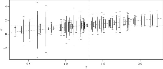
Adaptive, standard and empirical Bayes 95% confidence intervals for the radon dataset: the empirical Bayes intervals are plotted as wide grey lines and the adaptive intervals as narrow black lines, and the horizontal bars represent the endpoints of the standard intervals; vertical and horizontal lines are drawn at |$\sum \bar y_j/p$|⁠.

Also displayed in Fig. 2 are empirical Bayes intervals of the form |$\hat \theta_j \pm t_{1-\alpha/2 } \times (1/\hat \tau_{-j}^2 +n_j/ s^2_j )^{-1/2}$|⁠, where the empirical Bayes estimator is |$\hat\theta_j = (\hat \mu_{-j}/ \hat \tau_{-j}^2 + \bar y_j n_j/ s_j^2)/ ( 1/\hat\tau_j^2 + n_j/ s_j^2 )$| and |$t_{1-\alpha/2}$| is the |$1-\alpha/2$| quantile of the |$t_{n_j-1}$| distribution. As discussed in § 1, such intervals are always narrower than the corresponding standard intervals. For the radon data, they were narrower than the adaptive intervals for 46 of the 82 counties, although about 2% wider on average across counties. However, unlike the adaptive and standard intervals, the empirical Bayes intervals do not have constant coverage: the actual coverage rate of an empirical Bayes interval for a group |$j$| will depend on the unknown value of |$\theta_j$|⁠. We explore this further in the next subsection.

4.2. Risk performance and comparison with posterior intervals

Assuming within-group normality, the adaptive interval procedure described above has 95% coverage for each group |$j$| and for all values of |$\theta_1,\ldots, \theta_p$|⁠. Furthermore, the procedure is designed to approximately minimize the expected risk under the normal hierarchical model among all 95% confidence interval procedures. However, one may wonder how well the adaptive procedure works for fixed values of |$\theta_1,\ldots, \theta_p$|⁠. This question is particularly relevant in cases where the hierarchical model is misspecified, or when a hierarchical model is not appropriate, for example if the groups are not sampled. We investigate this for the radon data with a simulation study in which we take the county-specific sample means and variances as the true county-specific values, that is, we set |$\theta_j = \bar y_j$| and |$\sigma^2_j = s_j^2$| for each county |$j$|⁠. We then simulate |$n_j$| observations for each county |$j$| from the model |$Y_{i,j} \sim N(\theta_j,\sigma^2_j)$|⁠, independently within and across groups.

We generated 25 000 such simulated datasets. For each dataset, we computed the widths of the 95% adaptive, standard and empirical Bayes confidence intervals for each county having a sample size greater than 1. The results of this simulation study are displayed in Fig. 3. Panel (a) shows the expected widths of the adaptive and empirical Bayes procedures relative to those of the standard procedure. Based on the 25 000 simulated datasets, the estimated expected widths across counties were about 2|$\cdot$|28, 1|$\cdot$|60 and 1|$\cdot$|61 for the standard, adaptive and empirical Bayes procedures, respectively. As with the actual interval widths for the nonsimulated data, expected widths of the adaptive intervals are smaller than those of the standard intervals for 79 out of 82 counties. The empirical Bayes intervals are always narrower than the standard intervals for all groups by construction. However, while they tend to be narrower than the adaptive intervals for |$\theta_j$| far from |$\bar\theta=\sum_{j=1}^p \theta_j/p$|⁠, near this average they are often wider than the adaptive intervals. This is not too surprising, as the adaptive intervals are at their narrowest near this overall average, while the empirical Bayes intervals tend to over-cover here. This is illustrated in Fig. 3(b), which shows how the empirical Bayes credible intervals do not have constant coverage across groups, because they are centred around biased estimates that are shrunk towards the estimated overall mean |$\bar \theta$|⁠. If |$\theta_j$| is far from |$\bar\theta$| then the bias is high and the coverage too low, whereas if |$\theta_j$| is near |$\bar\theta$| then the coverage is too high since the variability of the shrinkage estimate |$\hat\theta_j$| is lower than that of |$\bar y_j$|⁠. The group-specific coverage rates of these intervals vary from about 91% to 98%, although the average coverage rate across groups is approximately 95%. In summary, the standard procedure has constant |$1-\alpha$| coverage across groups, but has wider intervals than those obtained from the adaptive and empirical Bayes procedures. The empirical Bayes procedure has narrower intervals but nonconstant coverage. The adaptive procedure has both narrower intervals and constant coverage.

Fig. 3.

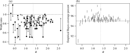
Simulation results: (a) expected interval widths of the adaptive (black) and empirical Bayes (grey) procedures, relative to the standard procedure; (b) empirical Bayes coverage rates, which can be seen to be nonconstant across groups. Error bars are 95% Clopper–Pearson intervals for the coverage rates, based on 25 000 simulated datasets; vertical lines are drawn at |$\sum \theta_j/p$| in each panel.

5. Discussion

Like standard |$t$|-intervals, the coverage properties of our adaptive intervals are based on the assumption that |$n^{1/2} (\bar Y_j - \theta_j)/S_j$| has a |$t$| distribution. Therefore, in terms of coverage rates, the robustness of these adaptive intervals with respect to deviations from within-group normality will be similar to the robustness of the standard |$t$|-interval. On the other hand, if the within-group distributions are normal but the across-group distribution is not, then the adaptive procedure will still maintain the chosen constant coverage rate but will not be optimal. We speculate that in such cases, the adaptive procedure based on a hierarchical normal model, while not optimal, will still asymptotically dominate the standard procedure in terms of risk, because the standard procedure is a limiting case of the adaptive procedure as the across-group variance goes to infinity.

The basic idea behind the adaptive procedure could be implemented with alternative models describing across-group heterogeneity, such as multivariate models that assume a nonexchangeable relationship among the group-level parameters. For example, given spatial information of the counties in the radon example, we could construct a |$w$|-function for each county that depends on data from spatially proximal counties. Such a |$w$|-function would result from using a spatial autoregressive model for the group-level parameters. Another extension would be to use a nonnormal across-group model for the group-level parameters. However, if the within-group and across-group models are not conjugate, then obtaining the Bayes-optimal intervals may require numerical integration and optimization.

Adaptive confidence intervals may also be constructed for contrasts between groups or other linear combinations of parameters. For example, if we are interested in |$\delta_{j,k} = \theta_j - \theta_k$|⁠, then we can construct an adaptive interval from |$\skew3\bar{d}_{j,k} = \bar y_j -\bar y_k$| based on |$\skew3\bar{d}_{j,k} \sim N( \delta_{j,k} , 2 \sigma^2/n )$| and use the model |$\delta_{j,k} \sim N(0 ,2\tau^2)$| to form the |$w$|-function. As long as the estimate of |$\tau^2$| used to form the |$w$|-function is not based on data from group |$j$| or group |$k$|⁠, then such an adaptive procedure will have |$1-\alpha$| constant coverage.

Acknowledgement

We thank the editor, associate editor and reviewers for their consideration of and comments on our paper. This research was supported by the U.S. National Science Foundation.

Supplementary material

Supplementary material available at Biometrika online includes replication code for the numerical results in this article.

Appendix

 

Proof of Proposition 3.

Without loss of generality we give a proof for the case where |$\mu = 0$| and |$\sigma^2 = 1$|⁠. The Bayes-optimal procedure minimizes the Bayes risk |$R(\psi ,C_w) = \int {\rm pr}\{ Y\in A(\theta) \} \, {\rm d}\theta$|⁠, where |$Y\sim N(0,1+\tau ^2)$|⁠. For a given |$w$|-function, the Bayes risk is

\[ R(\psi ,C_w) = \int_{\mathbb{R}} \Phi \!\left [ \frac{\theta- \Phi^{-1}\{\alpha(1-w)\}}{(1+\tau ^2)^{1/2}} \right ] - \Phi\!\left [ \frac{\theta - \Phi^{-1}(1-\alpha w)}{(1+\tau ^2)^{1/2}} \right ] {\rm d}\theta\text{.} \]

For fixed |$\theta$|⁠, let |$H(w)$| denote the integrand as a function of |$w$|⁠. Then

\begin{align*} H'(w) & = \exp\!\left (-\frac{1}{2}\frac{[ \theta - \Phi^{-1}\{\alpha(1-w)\}]^2}{1+\tau ^2}\right )\frac{1}{(1+\tau ^2)^{1/2}}\,\frac{\alpha}{\exp(-\frac{1}{2}[\Phi^{-1}\{\alpha(1-w)\}]^2)}\\ & \quad -\exp\!\left[ -\frac{1}{2} \frac{\{\theta - \Phi^{-1}(1-\alpha w\}^2}{1+\tau ^2}\right ]\frac{1}{(1+\tau ^2)^{1/2}}\,\frac{\alpha}{\exp[-\frac{1}{2}\{\Phi^{-1}(1-\alpha w)\}^2]}\text{.} \end{align*}

Setting |$H'(w)=0$| and simplifying shows that a critical point satisfies |${2\theta }/{\tau ^2} = \Phi^{-1}(w\alpha) - \Phi^{-1}\{(1-w)\alpha\} \equiv g(w)$|⁠. It is not difficult to verify that |$g(w)$| is a continuous and strictly increasing function of |$w$|⁠, with range |$(-\infty, \infty)$|⁠. Thus, for each |$\theta$| there is a unique solution to |$H'(w)=0$|⁠, given by |$w_{\psi}(\theta) = g^{-1}({2\theta / \tau ^2})$|⁠, which is a continuous and strictly increasing function of |$\theta$|⁠. Since |$H'(w)$| is continuous on |$[0,1]$| with only one root, and |$\lim_{w \rightarrow 0} H'(w)= -\infty$| and |$\lim_{w \rightarrow 1} H'(w) = \infty$|⁠, we have that |$H(w)$| is minimized by |$w_{\psi}(\theta)$|⁠. Therefore |$w_{\psi}(\theta)$| minimizes the Bayes risk, and |$C_{w_{\psi}}$| is the Bayes-optimal procedure. □

 

Proof of Proposition 4.

We can write |$C_w(y) = \{ \theta : y< \theta - \sigma l(\theta) , \, \theta - \sigma u(\theta) < y \}$|⁠. Letting |$f_1(\theta) = \theta - \sigma u(\theta)$| and |$f_2(\theta) = \theta - \sigma l(\theta)$|⁠, we first prove that |$C_w(y)$| can also be written as |$C_w(y) = \{ \theta : f_2^{-1}(y)<\theta < f_1^{-1}(y) \}$|⁠. Both |$\Phi^{-1}$| and |$w(\theta)$| are continuous nondecreasing functions. Therefore |$f_1(\theta) = \theta - \Phi^{-1} \{ 1-\alpha w(\theta)\}$| is a strictly increasing continuous function, with |$\lim_{\theta \to -\infty} \theta - \Phi^{-1} \{ 1-\alpha w(\theta)\} = -\infty$| and |$\lim_{\theta \to +\infty} \theta - \Phi^{-1} \{ 1-\alpha w(\theta)\}= +\infty$|⁠. Hence |$f_1^{-1}$| exists and is a strictly increasing continuous function with range |$(-\infty, \infty)$|⁠. Thus |$f_1(\theta) < y$| can also be expressed as |$\theta < f_1^{-1}(y)$|⁠. Similarly, |$y < f_2(\theta) $| can be expressed as |$ f_2^{-1}(y) < \theta$|⁠. Next, in order to show that |$C_w(y)$| is an interval, we need to show that |$f_2^{-1}(y) < f_1^{-1}(y)$|⁠. To see this, we only need to verify that |$ \theta - \sigma \Phi^{-1}\{1-\alpha w(\theta)\} < \theta - \sigma \Phi^{-1}[\alpha\{1-w(\theta)\}]$| or, equivalently, |$\Phi^{-1}\{\alpha w(\theta)\} < \Phi^{-1}[1-\alpha\{1-w(\theta)\}]$|⁠. This follows since |$\Phi^{-1}(x)$| is strictly increasing. Thus |$C_w(y) = \{ \theta : f_2^{-1}(y)<\theta < f_1^{-1}(y) \}$|⁠, which is an interval. □

 

Proof of Propositions 5 and 6.

These proofs are essentially the same as those of Propositions 2 and 4. □

 

Proof of Proposition 8.

For notational convenience, we write the |$\alpha$|-quantile of the |$t_q$| distribution as |$t_q(\alpha)$|⁠. We first prove a lemma bounding the width of the adaptive |$t$|-interval.

 

Lemma A1.

The width of |$C_{w_{\psi }}(\bar y, s^2)$| is less than |$|\bar y-\mu| + sn^{-1/2}\{ |t_q(\alpha/2)|+|t_q(1-\alpha/2)|\}$|⁠.

 

Proof.

The endpoints |$\theta^{\rm L}$| and |$\theta^{\rm U}$| of |$C_{w_{\psi}}(\bar y, s^2)$| solve |$ \theta^{\rm U} - sn^{-1/2}t_q\{1- \alpha w_{\psi}(\theta^{\rm U}) \}=\bar y $| and |$\theta^{\rm L} - sn^{-1/2}t[\alpha \{1-w_{\psi }(\theta^{\rm L})\}] =\bar y\text{.} $| Here |$w_{\psi }(\theta)$| is defined as |$w_{\psi }(\theta) = g^{-1} \{ 2\sigma(\theta-\mu)/\tau^2 \}$|⁠, where |$g(w) = \Phi^{-1}(\alpha w) - \Phi^{-1}\{\alpha(1-w) \}$|⁠. At the upper endpoint, we have |$w_{\psi}(\theta^{\rm U}) = F\{n^{1/2}(\bar y-\theta^{\rm U})/s\} /\alpha$|⁠, where |$F$| is the |$t_q$| cumulative distribution function. When |$\theta^{\rm U} > \mu$|⁠, we have |$w_{\psi}(\theta^{\rm U}) > g^{-1}(0) = 1/2$|⁠. Thus |$\theta^{\rm U} < \bar y - sn^{-1/2}t_q(\alpha/2)$|⁠. Also, |$g^{-1} \{ 2\sigma(\theta^{\rm U}-\mu)/\tau^{2}\} < 1$|⁠, so |$\theta^{\rm U} > \bar y - sn^{-1/2}t_q(\alpha)$|⁠. When |$\theta^{\rm U} < \mu$|⁠, |$\:\bar y - sn^{-1/2}t_q(\alpha/2)< \theta^{\rm U}$|⁠. This implies that |$\bar y - sn^{-1/2}t_q( \alpha)< \theta^{\rm U} < \bar y - sn^{-1/2}t_q( \alpha /2 ) $| if |$ \theta^{\rm U} > \mu$| and |$\bar y - sn^{-1/2}t_q( \alpha /2)< \theta^{\rm U} <\mu $| otherwise. Similarly, we have |$ \mu <\theta^{\rm L} < \bar y - sn^{-1/2}t_q(1 - \alpha /2 ) $| if |$ \theta^{\rm L} > \mu$| and |$ \bar y - sn^{-1/2}t_q(1 - \alpha /2)<\theta^{\rm L} < y - sn^{-1/2}t_q(1 - \alpha ) $| otherwise. Therefore

\begin{equation*} |C_{w_\psi}(\bar y,s ) | =\theta^{\rm U} - \theta^{\rm L} < |\bar y-\mu| + sn^{-1/2}\{ |t_q(\alpha/2)|+|t_q(1-\alpha/2)|\} \end{equation*}

as claimed. □

We now prove Proposition 8. That |$C_{w_{\hat \psi}}$| is a |$1-\alpha$| procedure follows by construction of the interval and from the fact that |$\hat \psi$| is independent of |$\bar Y$| and |$S^2$|⁠. To prove the convergence of the risk, let the endpoints of the oracle procedure be |$\theta^{\rm U}$| and |$\theta^{\rm L}$|⁠, which are the solutions to |$\theta^{\rm U} - \sigma n^{-1/2}\Phi^{-1}\{1- \alpha w_{\psi}(\theta^{\rm U}) \}=\bar Y $| and |$ \theta^{\rm L} - \sigma n^{-1/2}\Phi^{-1}[ \alpha \{1-w_{\psi }(\theta^{\rm L})\}] =\bar Y$|⁠. We denote the endpoints of |$C_{w_{\hat \psi}}$| by |$\theta^{\rm U}_q$| and |$\theta^{\rm L}_q$|⁠, which are the solutions to |$ \theta^{\rm U}_q - Sn^{-1/2}t_q\{ 1-\alpha w_{\hat \psi}(\theta^{\rm U}_q) \}=\bar Y $| and |$ \theta^{\rm L}_q - Sn^{-1/2}t_q[ \alpha \{1-w_{\hat \psi }(\theta^{\rm L}_q)\}] =\bar Y$|⁠. We first prove that |$|C_{w_{\hat \psi}}|-|C_{w_{ \psi}}| = (\theta^{\rm U}_q - \theta^{\rm U}) + (\theta^{\rm L} - \theta^{\rm L}_q) \rightarrow 0$| almost surely as |$q \to \infty$| for each fixed |$\bar Y$|⁠. We can write the upper endpoints as |$\theta^{\rm U} = G(\psi, \bar Y, \sigma^2)$|} and |$\theta^{\rm U}_q = G_q(\hat \psi, \bar Y, S^2)$|⁠, where |$G$| and |$G_q$| are continuous functions of their parameters. The difference between |$G$| and |$G_q$| is that the former is obtained based on |$z$|-quantiles, while the latter is based on |$t$|-quantiles. We have

\begin{align} |\theta^{\rm U}_q - \theta^{\rm U}| &=|G_q(\hat \psi, \bar Y, S^2) - G(\psi, \bar Y, \sigma^2)| \nonumber \\ & \leqslant |G_q(\hat \psi, \bar Y, S^2) - G(\hat \psi, \bar Y, S^2)| + |G(\hat \psi, \bar Y, S^2) - G(\psi, \bar Y, \sigma^2)|\text{.} \end{align}

(A1)

The first term in (A1) converges to zero because the convergence of |$G_q \to G$| is uniform, and the second term converges to zero because |$(\hat \psi, S^2) \rightarrow (\psi,\sigma^2)$| almost surely. Elaborating on the convergence of the first term, note that |$G_q$| is a monotone sequence of continuous functions: given |$q_2 > q_1$|⁠, we have |$t_{q_2}(1-\alpha w) < t_{q_1}(1- \alpha w)$|⁠; hence |$\theta - Sn^{-1/2}t_{q_2}\{1-\alpha w_{\hat \psi}(\theta)\} > \theta - Sn^{-1/2}t_{q_1}\{1-\alpha w_{\hat \psi}(\theta)\}$| and so |$G_{q_2}(\hat \psi, \bar Y, S^2) < G_{q_1}(\hat \psi, \bar Y, S^2)$|⁠. Therefore, by Dini’s theorem, |$G_q \rightarrow G$| uniformly on a compact set of |$(\hat \psi,S^2)$| values. Since |$(\hat \psi, S^2) \rightarrow (\psi,\sigma^2)$| almost surely, with probability 1 there is an integer |$Q$| such that when |$q> Q$|⁠, |$\:|\hat \psi -\psi| \leqslant c_1$| and |$|S^2 - \sigma^2| \leqslant c_2$| for any two positive constants |$c_1$| and |$c_2$|⁠. Thus, |$G_q$| converges to |$G$| uniformly on this compact set and the first term in (A1) converges to zero.

Now we show that the expected width converges to the oracle width by integrating over |$\bar Y$|⁠. This is done by finding a dominating function for |$| C_{w_{\hat\psi}}(\bar Y, S^2)|$| and applying the dominated convergence theorem. By the previous lemma we know that

\begin{equation*} |C_{w_{\hat \psi }}(\bar Y, S^2) | < |\bar Y|+ |\hat \mu| + Sn^{-1/2}\{ |t_q(\alpha/2)|+|t_q(1-\alpha/2)|\}\text{.} \end{equation*}

Note that |$|t_q(\alpha/2)|+|t_q(1-\alpha/2)| < |t_1(\alpha/2)|+|t_1(1-\alpha/2)|$|⁠, where |$t_1$| is the |$t$|-quantile with one degree of freedom. Similar to the argument earlier in this proof, given two constants |$c_1, c_2 > 0$|⁠, we can find a |$Q$| such that when |$q > Q$| we have |$|\hat \mu |<| \mu| + c_1$| and |$S^2 < \sigma^2 + c_2$| almost surely. This gives a dominating function for |$|C_{w_{\hat \psi }}(\bar Y, S^2) |$|⁠,

\begin{equation*} |C_{w_{\hat \psi }}(\bar Y, S^2) | < \bar W(\bar Y, S^2,\hat \psi ) = |\bar Y| + |\mu| + c_1 + n^{-1/2}(\sigma^2+c_2)^{1/2}\{ |t_1(\alpha/2)|+|t_1(1-\alpha/2)|\}\text{.} \end{equation*}

Since |$|\bar Y|$| is a folded normal random variable with finite mean, it is easy to see that this dominating function is integrable. Therefore, by the dominated convergence theorem we have |$ \lim_{q\rightarrow \infty} {E}{ | C_{w_{\hat\psi}}|} = {E}{ | C_{w_{\psi}}|}$|⁠, which completes the proof of Proposition 8. □

Author notes