Variance estimation in the particle filter

Summary

This paper concerns numerical assessment of Monte Carlo error in particle filters. We show that by keeping track of certain key features of the genealogical structure arising from resampling operations, it is possible to estimate variances of a number of Monte Carlo approximations that particle filters deliver. All our estimators can be computed from a single run of a particle filter. We establish that, as the number of particles grows, our estimators are weakly consistent for asymptotic variances of the Monte Carlo approximations and some of them are also non-asymptotically unbiased. The asymptotic variances can be decomposed into terms corresponding to each time step of the algorithm, and we show how to estimate each of these terms consistently. When the number of particles may vary over time, this allows approximation of the asymptotically optimal allocation of particle numbers.

1. Introduction

Particle filters, or sequential Monte Carlo methods, provide approximations of integrals with respect to sequences of measures. In popular statistical inference applications, these measures arise naturally from conditional distributions in hidden Markov models, or are constructed artificially to bridge between target distributions in Bayesian analysis. The number of particles used controls the trade-off between computational complexity and accuracy. Theoretical properties of this relationship have been the subject of intensive research; the literature includes central limit theorems (Del Moral & Guionnet, 1999; Chopin, 2004; Künsch, 2005; Douc & Moulines, 2008) and a variety of refined asymptotic (Douc et al., 2005; Del Moral et al., 2007) and non-asymptotic (Del Moral & Miclo, 2001; Cérou et al., 2011) results. These studies provide a wealth of insight into the mathematical behaviour of particle filter approximations and validate them theoretically, but considerably less is known about how, in practice, to extract information from a realization of a single particle filter in order to report numerical measures of Monte Carlo error. This is in notable contrast to other families of Monte Carlo techniques, especially Markov chain Monte Carlo, for which an extensive literature on variance estimation exists. Our main aim is to address this gap.

We introduce particle filters via a framework of Feynman–Kac models (Del Moral, 2004). This allows us to identify the key ingredients of particle filters and the measures they approximate. Based on a single realization of a particle filter, we provide unbiased estimators of the variance and individual asymptotic variance terms for a class of unnormalized particle approximations. No estimators of these quantities based on a single run of a particle filter have previously appeared in the literature, and all of our estimators ultimately arise from particle approximations of quantities appearing in a non-asymptotic second-moment expression. Upon suitable rescaling, we establish that our estimators are weakly consistent for asymptotic variances associated with a larger class of particle approximations. One of these rescaled estimators is closely related to that of Chan & Lai (2013), which is the only other consistent asymptotic variance estimator based on a single realization of a particle filter in the literature. We also demonstrate how one can use the estimators to inform the choice of algorithm parameters in an attempt to improve performance.

2. Particle filters

2.1. Notation and conventions

For a generic measurable space |$(\mathsf{E},\mathcal{E})$|⁠, we denote by |$\mathcal{L}(\mathcal{E})$| the set of |$\mathbb{R}$|-valued, |$\mathcal{E}$|-measurable and bounded functions on |$\mathsf{E}$|⁠. For |$\varphi\in\mathcal{L}(\mathcal{E})$|⁠, |$\mu$| a measure and |$K$| an integral kernel on |$(\mathsf{E},\mathcal{E})$|⁠, we write |$\mu(\varphi)=\int_{\mathsf{E}}\varphi(x)\mu({\rm d}x)$|⁠, |$K(\varphi)(x)=\int_{\mathsf{E}}K(x,{\rm d}x^{\prime})\varphi(x^{\prime})$| and |$\mu K(A)=\int_{\mathsf{E}}\mu({\rm d}x)K(x,A)$|⁠. Constant functions |$x\in E\mapsto c\in\mathbb{R}$| are denoted simply by |$c$|⁠. For |$\varphi\in\mathcal{L}(\mathcal{E})$|⁠, |$\varphi^{\otimes2}(x,x^{\prime})=\varphi(x)\varphi(x^{\prime})$|⁠. The Dirac measure located at |$x$| is denoted by |$\delta_{x}$|⁠. For any sequence |$(a_{n})_{n\in\mathbb{Z}}$| and |$p\leq q$|⁠, |$a_{p:q}=(a_{p},\ldots,a_{q})$| and by convention |$\prod_{p=0}^{-1}a_{p}=1$|⁠. For any |$m\in\mathbb{N}$|⁠, |$[m]=\{1,\ldots,m\}$|⁠. For any |$c\in\mathbb{R}$|⁠, |$\lceil c\rceil$| is the smallest integer greater than or equal to |$c$|⁠. For a vector of positive values |$(a_{1},\ldots,a_{m})$|⁠, we denote by |$\mathcal{C}(a_{1},\ldots,a_{m})$| the categorical distribution over |$\{1,\ldots,m\}$| with probabilities |$(a_{1}/\sum_{i=1}^{m}a_{i},\ldots,a_{m}/\sum_{i=1}^{m}a_{i})$|⁠. When a random variable is indexed by a superscript |$N$|⁠, a sequence of such random variables is implicitly defined by considering each value |$N\in\mathbb{N}$|⁠, and limits will always be taken along this sequence.

2.2. Discrete time Feynman–Kac models

On a measurable space |$\left(\mathsf{X},\mathcal{X}\right)$| with |$n$| a nonnegative integer, let |$M_{0}$| be a probability measure, |$M_{1},\ldots,M_{n}$| a sequence of Markov kernels and |$G_{0},\ldots,G_{n}$| a sequence of |$\mathbb{R}$|-valued, strictly positive, upper-bounded functions. We assume throughout that |$\mathsf{X}$| does not consist of a single point. We define a sequence of measures by |$\gamma_{0}=M_{0}$| and, recursively,

\begin{equation} \gamma_{p}(S)=\int_{\mathsf{X}}\gamma_{p-1}({\rm d}x)G_{p-1}(x)M_{p}(x,S),\qquad p\in[n],\quad S\in\mathcal{X}\text{.}\label{eq:gamman} \end{equation}

(1)

Since |$\gamma_{p}(\mathsf{X})\in(0,\infty)$| for each |$p$|⁠, the following probability measures are well-defined:

\begin{equation} \eta_{p}(S)=\frac{\gamma_{p}(S)}{\gamma_{p}(\mathsf{X})},\qquad p\in\{0,\ldots,n\},\quad S\in\mathcal{X}\text{.}\label{eq:etan} \end{equation}

(2)

The representation |$\gamma_{n}(\varphi)=E\{\varphi(X_{n})\prod_{p=0}^{n-1}G_{p}(X_{p})\}$|⁠, where the expectation is taken with respect to the Markov chain with initial distribution |$X_{0}\sim M_{0}$| and transitions |$X_{p}\sim M_{p}(X_{p-1},\cdot)$|⁠, establishes the connection to Feynman–Kac formulae. Measures with the structure in (1)–(2) arise in a variety of statistical contexts.

2.3. Motivating examples of Feynman–Kac models

As a first example, consider a hidden Markov model: a bivariate Markov chain |$(X_{p},Y_{p})_{p=0,\ldots,n}$| where |$(X_{p})_{p=0,\ldots,n}$| is itself Markov with initial distribution |$M_{0}$| and transitions |$X_{p}\sim M_{p}(X_{p-1},\cdot)$|⁠, and such that each |$Y_{p}$| is conditionally independent of |$(X_{q},Y_{q};q\neq p)$| given |$X_{p}$|⁠. If the conditional distribution of |$Y_{p}$| given |$X_{p}$| admits a density |$g_{p}(X_{p},\cdot)$| and one fixes a sequence of observed values |$y_{0},\ldots,y_{n-1}$|⁠, then with |$G_{p}(x_{p})=g_{p}(x_{p},y_{p})$|⁠, |$\eta_{n}$| is the conditional distribution of |$X_{n}$| given |$y_{0},\ldots,y_{n-1}$|⁠. Hence, |$\eta_{n}(\varphi)$| is a conditional expectation and |$\gamma_{n}(\mathsf{X})=\gamma_{n}(1)$| is the marginal likelihood of |$y_{0},\ldots,y_{n-1}$|⁠.

As a second example, consider the following sequential simulation set-up. Let |$\pi_{0}$| and |$\pi_{1}$| be two probability measures on |$\left(\mathsf{X},\mathcal{X}\right)$| such that |$\pi_{0}({\rm d}x)=\bar{\pi}_{0}(x)\,{\rm d}x/Z_{0}$| and |$\pi_{1}({\rm d}x)=\bar{\pi}_{1}(x)\,{\rm d}x/Z_{1}$|⁠, where |$\bar{\pi}_{0}$| and |$\bar{\pi}_{1}$| are unnormalized probability densities with respect to a common dominating measure |${\rm d}x$| and |$Z_{i}=\int_{\mathsf{X}}\bar{\pi}_{i}(x)\,{\rm d}x$|⁠, |$i\in\{0,1\}$|⁠, are integrals unavailable in closed form. In Bayesian statistics |$\pi_{1}$| may arise as a badly behaved posterior distribution from which one wishes to sample, |$\pi_{0}$| is a more benign distribution from which sampling is feasible, and calculating |$Z_{1}/Z_{0}$| allows assessment of model fit. Introducing a sequence |$0=\beta_{0}<\cdots<\beta_{n}=1$| and taking |$G_{p}(x)=\left\{ \bar{\pi}_{1}(x)/\bar{\pi}_{0}(x)\right\} ^{\beta_{p+1}-\beta_{p}}$|⁠, |$M_{0}=\pi_{0}$| and, for each |$p=1,\ldots,n$|⁠, |$M_{p}$| as a Markov kernel invariant with respect to the distribution with density proportional to |$\bar{\pi}_{0}(x)^{1-\beta_{p}}\bar{\pi}_{1}(x)^{\beta_{p}}$|⁠, elementary manipulations yield

\[ \gamma_{p}(S)=\frac{1}{Z_{0}}\int_{S}\bar{\pi}_{0}(x)^{1-\beta_{p}}\bar{\pi}_{1}(x)^{\beta_{p}}\,{\rm d}x,\quad\eta_{n}=\pi_{1},\quad\gamma_{n}(\mathsf{X})=\frac{Z_{1}}{Z_{0}}, \]

so that |$\eta_{1},\ldots,\eta_{n-1}$| forms a sequence of intermediate distributions between |$\pi_{0}$| and |$\pi_{1}$|⁠. This type of construction appears in Del Moral et al. (2006) and references therein.

2.4. Particle approximations

We now introduce particle approximations of the measures in (1)–(2). Let |$c_{0:n}$| be a sequence of positive real numbers and let |$N\in\mathbb{N}$|⁠. We define a sequence of particle numbers |$N_{0:n}$| by |$N_{p}=\lceil c_{p}N\rceil$| for |$p\in\{0,\ldots,n\}$|⁠. To avoid notational complications, we shall assume throughout that |$c_{0:n}$| and |$N$| are such that |$\text{min}_{p}N_{p}\geq2$|⁠. The particle system consists of a sequence |$\zeta=\zeta_{0:n}$| where for each |$p$|⁠, |$\zeta_{p}=(\zeta_{p}^{1},\ldots,\zeta_{p}^{N_{p}})$| and each |$\zeta_{p}^{i}$| is valued in |$\mathsf{X}$|⁠. To describe the resampling operation we also introduce random variables denoting the indices of the ancestors of each random variable |$\zeta_{p}^{i}$|⁠. That is, for each |$i\in[N_{p}]$|⁠, |$A_{p-1}^{i}$| is a |$[N_{p-1}]$|-valued random variable and we write |$A_{p-1}=(A_{p-1}^{1},\ldots,A_{p-1}^{N_{p}})$| for |$p\in[n]$| and |$A=A_{0:n-1}$|⁠.

A simple description of the particle system is given in Algorithm 1. An important and non-standard feature is that we keep track of a collection of indices |$E_{0:n}$| with |$E_{p}=(E_{p}^{1},\ldots,E_{p}^{N_{p}})$| for each |$p$|⁠, which will be put to use in our variance estimators. We call these Eve indices because |$E_{p}^{i}$| represents the index of the time-|$0$| ancestor of |$\zeta_{p}^{i}$|⁠. The fact that |$N_{p}$| may vary with |$p$| is also atypical, and allows us to address asymptotically optimal particle allocation in § 5.1. On a first reading, one may wish to assume that |$N_{0:n}$| is not time-varying, i.e., |$c_{p}=1$| so |$N_{p}=N$| for all |$p\in\{0,\ldots,n\}$|⁠. Figure 1 is a graphical representation of a realization of a small particle system.

Fig. 1.

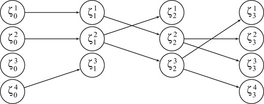
A particle system with |$n=3$| and |$N_{0:3}=(4,3,3,4)$|⁠. An arrow from |$\zeta_{p-1}^{i}$| to |$\zeta_{p}^{j}$| indicates that the ancestor of |$\zeta_{p}^{j}$| is |$\zeta_{p-1}^{i}$|⁠, i.e., |$A_{p-1}^{j}=i$|⁠. In the realization shown, the ancestral indices are |$A_{0}=(1,2,4)$|⁠, |$A_{1}=(2,1,2)$| and |$A_{2}=(3,2,2,3)$|⁠, while |$E_{0}=(1,2,3,4)$|⁠, |$E_{1}=(1,2,4)$|⁠, |$E_{2}=(2,1,2)$| and |$E_{3}=(2,1,1,2)$|⁠.

 

Algorithm 1.

The particle filter.

1. At time |$0$|⁠: for each |$i\in[N_{0}]$|⁠, sample |$\zeta_{0}^{i}\sim M_{0}(\cdot)$| and set |$E_{0}^{i}\leftarrow i$|⁠.

2. At each time |$p=1,\ldots,n$|⁠: for each |$i\in[N_{p}]$|⁠,

   • a.sample |$A_{p-1}^{i}\sim\mathcal{C}\{G_{p-1}(\zeta_{p-1}^{1}),\ldots,G_{p-1}(\zeta_{p-1}^{N_{p-1}})\}$|⁠.

   • b.sample |$\zeta_{p}^{i}\sim M_{p}(\zeta_{p-1}^{A_{p-1}^{i}},\cdot)$| and set |$E_{p}^{i}\leftarrow E_{p-1}^{A_{p-1}^{i}}$|⁠.

The particle approximations to |$\eta_{n}$| and |$\gamma_{n}$| are defined respectively by the random measures

\[ \eta_{n}^{N}=\frac{1}{N_{n}}\sum_{i\in[N_{n}]}\delta_{\zeta_{n}^{i}},\qquad\gamma_{n}^{N}=\left\{ \prod_{p=0}^{n-1}\eta_{p}^{N}(G_{p})\right\} \eta_{n}^{N}, \]

and we observe that, similar to (2), |$\eta_{n}^{N}=\gamma_{n}^{N}/\gamma_{n}^{N}(1)$|⁠. To simplify presentation, the dependence of |$\gamma_{n}^{N}$| and |$\eta_{n}^{N}$| on |$c_{0:n}$| is suppressed from the notation. The following proposition establishes basic properties of the particle approximations, which validate their use.

 

Preposition 1.

There exists a map |$\sigma_{n}^{2}:\mathcal{L}(\mathcal{X})\rightarrow[0,\infty)$| such that for any |$\varphi\in\mathcal{L}(\mathcal{X})$|:

• (i)|$E\left\{ \gamma_{n}^{N}(\varphi)\right\} =\gamma_{n}(\varphi)$| for all |$N\geq1$|;

• (ii)|$\gamma_{n}^{N}(\varphi)\to\gamma_{n}(\varphi)$| almost surely and |$N{\rm var}\left\{ \gamma_{n}^{N}(\varphi)/\gamma_{n}(1)\right\} \to\sigma_{n}^{2}(\varphi)$|;

• (iii)|$\eta_{n}^{N}(\varphi)\to\eta_{n}(\varphi)$| almost surely and |$NE\left[\left\{ \eta_{n}^{N}(\varphi)-\eta_{n}(\varphi)\right\} ^{2}\right]\to\sigma_{n}^{2}\{\varphi-\eta_{n}(\varphi)\}$|.

If the number of particles is constant over time, |$N_{p}=N$|⁠, these properties are well known and can be deduced, for example, from various results of Del Moral (2004). The arguments used to treat the general |$N_{p}=\left\lceil c_{p}N\right\rceil$| case are not substantially different, but since they seem not to have been published anywhere in exactly the form we need, we include a proof of Proposition 1 in the Supplementary Material.

2.5. A variance estimator

For |$\varphi\in\mathcal{L}(\mathcal{X})$|⁠, consider the quantity

\begin{align} V_{n}^{N}(\varphi) & =\eta_{n}^{N}(\varphi)^{2}-\left(\prod_{p=0}^{n}\frac{N_{p}}{N_{p}-1}\right)\frac{1}{N_{n}^{2}}\sum_{i,j:E_{n}^{i}\neq E_{n}^{j}}\varphi(\zeta_{n}^{i})\varphi(\zeta_{n}^{j})\label{eq:V_n^N_defn_front}\\ \end{align}

(3)

\begin{align} & =\eta_{n}^{N}(\varphi)^{2}\left(1-\prod_{p=0}^{n}\frac{N_{p}}{N_{p}-1}\right)+\left(\prod_{p=0}^{n}\frac{N_{p}}{N_{p}-1}\right)\frac{1}{N_{n}^{2}}\sum_{i\in[N_{0}]}\sum_{j:E_{n}^{j}=i}\varphi(\zeta_{n}^{j})^{2},\label{eq:VnN_rearranged} \end{align}

(4)

which is readily computable as a byproduct of Algorithm 1. The following theorem is the first main result of the paper. We state it here to make some of the practical implications of our work accessible to the reader before entering into more technical details; it shows that via (3), the variables |$E_{n}^{i}$| can be used to estimate the Monte Carlo errors associated with |$\gamma_{n}^{N}(\varphi)$| and |$\eta_{n}^{N}(\varphi)$|⁠.

 

Theorem 1.

The following hold for any |$\varphi\in\mathcal{L}(\mathcal{X})$|⁠, with |$\sigma_{n}^{2}(\cdot)$| as in Proposition 1:

• (i)|$E\left\{ \gamma_{n}^{N}(1)^{2}V_{n}^{N}(\varphi)\right\} ={\rm var}\left\{ \gamma_{n}^{N}(\varphi)\right\}$| for all |$N\geq1$|;

• (ii)|$NV_{n}^{N}(\varphi)\to\sigma_{n}^{2}(\varphi)$| in probability;

• (iii)|$NV_{n}^{N}\{\varphi-\eta_{n}^{N}(\varphi)\}\to\sigma_{n}^{2}\{\varphi-\eta_{n}(\varphi)\}$| in probability.

 

Remark 1.

Since |$\eta_{n}^{N}\{\varphi-\eta_{n}^{N}(\varphi)\}=0$|⁠, the estimator |$NV_{n}^{N}\{\varphi-\eta_{n}^{N}(\varphi)\}$| simplifies to

\[ NV_{n}^{N}\left\{ \varphi-\eta_{n}^{N}(\varphi)\right\} =N\left(\prod_{p=0}^{n}\frac{N_{p}}{N_{p}-1}\right)\frac{1}{N_{n}^{2}}\sum_{i\in[N_{0}]}\sum_{j:E_{n}^{j}=i}\left\{ \varphi(\zeta_{n}^{j})-\eta_{n}^{N}(\varphi)\right\} ^{2}\text{.} \]

This estimator is a deterministic and asymptotically negligible modification of Chan & Lai’s (2013) weakly consistent estimator of |$\sigma_{n}^{2}\{\varphi-\eta_{n}(\varphi)\}$|⁠, given by

\[ \hat{\sigma}_{{\rm CL}}^{2}\{\varphi-\eta_{n}(\varphi)\}=\frac{1}{N}\sum_{i\in[N]}\sum_{j:E_{n}^{j}=i}\left\{ \varphi(\zeta_{n}^{j})-\eta_{n}^{N}(\varphi)\right\} ^{2}, \]

when |$N$| is not time-varying. Our estimator is larger than Chan and Lai’s due to the factor |$\prod_{p=0}^{n}N_{p}/(N_{p}-1)$|⁠; we find in the examples that there is little difference in the regime where both are nearly unbiased. Our main contributions, therefore, are the estimators proposed for which there are no existing alternatives in the literature: those with properties (i) or (ii) of Theorem 1, and those developed in the following sections to estimate individual asymptotic variance terms arising from a natural decomposition of |$\sigma_{n}^{2}(\varphi)$|⁠.

The proof of Theorem 1, given in the Appendix, relies on a number of intermediate results concerning moment properties of the particle approximations which we shall develop. Before embarking on this, we discuss how |$V_{n}^{N}(\varphi)$| may be interpreted. Consider independent, identically distributed random variables |$X_{1},\ldots,X_{N}$| with sample mean |$\bar{X}$|⁠. The unbiased estimator of the variance of |$\bar{X}$| is

\begin{equation} \frac{1}{N(N-1)}\sum_{i}(X_{i}-\bar{X})^{2}=\bar{X}^{2}\left(1-\frac{N}{N-1}\right)+\left(\frac{N}{N-1}\right)\frac{1}{N^{2}}\sum_{i=1}^{N}X_{i}^{2}\text{.}\label{eq:sample_varmean} \end{equation}

(5)

Observe the resemblance between the right-hand sides of (4) and (5): the role of |$X_{i}^{2}$| is played by |$\sum_{j:E_{n}^{j}=i}\varphi(\zeta_{n}^{j})^{2}$|⁠, the sum of |$\varphi^{2}$| evaluated at the descendants of |$\zeta_{0}^{i}$|⁠. This change, and the product term |$\prod_{p=0}^{n}N_{p}/(N_{p}-1)$| replacing |$N/(N-1)$|⁠, arise from the nontrivial dependence structure associated with |$\zeta_{0},\ldots,\zeta_{n}$|⁠. One of the main difficulties we face is to develop a suitable mathematical perspective from which to account for this dependence and establish Theorem 1.

The main statistical implication of Theorem 1 is that the variance estimators are weakly consistent as |$N\rightarrow\infty$| with |$n$| fixed. In the opposite regime, where |$N$| is fixed and |$n\rightarrow\infty$|⁠, the estimators degenerate because the resampling operations cause |$E_{n}^{1},\ldots,E_{n}^{N}$| to eventually become equal. Using results reported here, Olsson & Douc (2018) address the degeneracy issue by modifying |$\hat{\sigma}_{{\rm CL}}^{2}$| so that ancestries are traced only over a fixed time horizon.

3. Moment properties of the particle approximations

3.1. Genealogical tracing variables

Our next step is to introduce some auxiliary random variables associated with the genealogical structure of the particle system. These variables are introduced only for purposes of analysis: they will assist in deriving and justifying our variance estimators. Given |$(A,\zeta)$|⁠, the first collection of variables, |$K^{1}=(K_{0}^{1},\ldots,K_{n}^{1})$|⁠, is conditionally distributed as follows: |$K_{n}^{1}$| is uniformly distributed on |$[N_{n}]$| and for each |$p=n-1,\ldots,0$|⁠, |$K_{p}^{1}=A_{p}^{K_{p+1}^{1}}$|⁠. Given |$(A,\zeta)$| and |$K^{1}$|⁠, the second collection of variables, |$K^{2}=(K_{0}^{2},\ldots,K_{n}^{2})$|⁠, is conditionally distributed as follows: |$K_{n}^{2}$| is uniformly distributed on |$[N_{n}]$| and for each |$p=n-1,\ldots,0$| we have |$K_{p}^{2}=A_{p}^{K_{p+1}^{2}}$| if |$K_{p+1}^{2}\neq K_{p+1}^{1}$| and |$K_{p}^{2}\sim\mathcal{C}\{G_{p}(\zeta_{p}^{1}),\ldots,G_{p}(\zeta_{p}^{N_{p}})\}$| if |$K_{p+1}^{2}=K_{p+1}^{1}$|⁠. The interpretation of |$K^{1}$| is that it traces backwards in time the ancestral lineage of a particle chosen randomly from the population at time |$n$|⁠. The interpretation of |$K^{2}$| is slightly more complicated: it traces backwards in time a sequence of broken ancestral lineages, where breaks occur when components of |$K^{1}$| and |$K^{2}$| coincide.

3.2. Lack of bias and second moment of |$\gamma_{n}^{N}(\varphi)$|

We now give expressions for the first two moments of |$\gamma_{n}^{N}(\varphi)$|⁠.

 

Lemma 1.

For any |$\varphi\in\mathcal{L}(\mathcal{X})$|⁠, |$E\left\{ \gamma_{n}^{N}(1)\varphi(\zeta_{n}^{K_{n}^{1}})\right\} =\gamma_{n}(\varphi)$| and |$E\left\{ \gamma_{n}^{N}(\varphi)\right\} =\gamma_{n}(\varphi)$|.

The proof is in the Supplementary Material. The lack-of-bias property |$E\{ \gamma_{n}^{N}(\varphi)\} =\gamma_{n}(\varphi)$| is well known and a martingale proof for the |$N_{p}=N$| case can be found in Del Moral (2004, Ch. 9).

In order to present an expression for the second moment of |$\gamma_{n}^{N}(\varphi)$|⁠, we now introduce a collection of measures on |$\mathcal{X}^{\otimes2}$|⁠, denoted by |$\{\mu_{b}:b\in B_{n}\}$|⁠, where |$B_{n}=\{0,1\}^{n+1}$| is the set of binary strings of length |$n+1$|⁠. The measures are constructed as follows. For a given |$b\in B_{n}$|⁠, let |$(X_{p},X_{p}')_{p=0,\ldots,n}$| be a Markov chain with state space |$\mathsf{X}^{2}$|⁠, distributed according to the following recipe. If |$b_{0}=0$| then |$X_{0}\sim M_{0}$| and |$X_{0}'\sim M_{0}$| independently, while if |$b_{0}=1$| then |$X_{0}'=X_{0}\sim M_{0}$|⁠. Then, for |$p=1,\ldots,n$|⁠, if |$b_{p}=0$| then |$X_{p}\sim M_{p}(X_{p-1},\cdot)$| and |$X_{p}'\sim M_{p}(X_{p-1}',\cdot)$| independently, while if |$b_{p}=1$| then |$X_{p}'=X_{p}\sim M_{p}(X_{p-1},\cdot)$|⁠. Letting |$E_{b}$| denote expectation with respect to the law of this Markov chain, we then define

\[ \mu_{b}(S)=E_{b}\left[\mathbb{I}\left\{ (X_{n},X_{n}')\in S\right\} \prod_{p=0}^{n-1}G_{p}(X_{p})G_{p}(X_{p}')\right],\qquad S\in\mathcal{X}^{\otimes2},\; b\in B_{n}\text{.} \]

Recalling that |$\gamma_{n}(\varphi)=E\{\varphi(X_{n})\prod_{p=0}^{n-1}G_{p}(X_{p})\}$| for |$\varphi\in\mathcal{L}(\mathcal{X})$|⁠, we write |$\mu_{b}(\phi)=E_{b}\{ \phi(X_{n},X_{n}')\prod_{p=0}^{n-1}G_{p}(X_{p})G_{p}(X_{p}')\}$| for |$\phi\in\mathcal{L}(\mathcal{X}^{\otimes2})$| and |$b\in B_{n}$|⁠, and can view |$\mu_{b}$| as defining a Feynman–Kac model on |$\mathcal{X}^{\otimes2}$|⁠.

 

Remark 2.

Observe that with |$0_{n}\in B_{n}$| denoting the zero string, |$\mu_{0_{n}}(\varphi^{\otimes2})=\gamma_{n}(\varphi)^{2}$|⁠.

In order to succinctly express the second moment of |$\gamma_{n}^{N}(\varphi)$|⁠, we define appropriate sets of pairs of strings of length |$n+1$|⁠. Letting |$[N_{0:n}]=[N_{0}]\times\cdots\times[N_{n}]$| and, for any |$b\in B_{n}$|⁠,

\[ \mathcal{I}(b)=\{(k^{1},k^{2})\in[N_{0:n}]^{2}\,:\,\text{for each }p,\:k_{p}^{1}=k_{p}^{2}\iff b_{p}=1\}, \]

we have that |$\mathcal{I}(b)$| contains strings which coincide in their |$p$|th coordinate exactly when |$b_{p}=1$|⁠.

 

Lemma 2.

For any |$\phi\in\mathcal{L}(\mathcal{X}^{\otimes2})$|⁠, |$\varphi\in\mathcal{L}(\mathcal{X})$| and |$b\in B_{n}$|,

\begin{equation} E\left[\mathbb{I}\left\{ (K^{1},K^{2})\in\mathcal{I}(b)\right\} \gamma_{n}^{N}(1)^{2}\phi(\zeta_{n}^{K_{n}^{1}},\zeta_{n}^{K_{n}^{2}})\right]=\prod_{p=0}^{n}\left\{ \left(\frac{1}{N_{p}}\right)^{b_{p}}\left(1-\frac{1}{N_{p}}\right)^{1-b_{p}}\right\} \mu_{b}(\phi)\label{eq:second_moment_formula_disintegrated} \end{equation}

(6)

and

\begin{equation} E\left\{ \gamma_{n}^{N}(\varphi)^{2}\right\} =\sum_{b\in B_{n}}\prod_{p=0}^{n}\left(\frac{1}{N_{p}}\right)^{b_{p}}\left(1-\frac{1}{N_{p}}\right)^{1-b_{p}}\mu_{b}(\varphi^{\otimes2})\text{.}\label{eq:second_moment_formula} \end{equation}

(7)

The proof of Lemma 2 uses an argument involving the law of a doubly conditional sequential Monte Carlo algorithm (see alsoAndrieu et al., 2018). The identity (7) was first proved by Cérou et al. (2011) in the case where |$N_{p}=N$|⁠. Our proof technique is different: we obtain (7) as a consequence of (6). The appearance of |$K^{1}$| and |$K^{2}$| in (6) is also central to the justification of our variance estimators below.

3.3. Asymptotic variances

For each |$p\in\{0,\ldots,n\}$|⁠, let |$e_{p}\in B_{n}$| denote the vector with a |$1$| in position |$p$| and zeros elsewhere. As in Remark 2, |$0_{n}$| denotes the zero string in |$B_{n}$|⁠. The following result builds upon Lemmas 1 and 2. It shows that a particular subset of the measures |$\{\mu_{b}:b\in B_{n}\}$|⁠, namely |$\mu_{0_{n}}$| and |$\{\mu_{e_{p}}:p=0,\ldots,n\}$|⁠, appear in the asymptotic variances; its proof is in the Supplementary Material.

 

Lemma 3.

Let, for any |$\varphi\in\mathcal{L}(\mathcal{X})$|,

\begin{equation} v_{p,n}(\varphi)=\frac{\mu_{e_{p}}(\varphi^{\otimes2})-\mu_{0_{n}}(\varphi^{\otimes2})}{\gamma_{n}(1)^{2}},\qquad p\in\{0,\ldots,n\}\text{.}\label{eq:vpndefn} \end{equation}

(8)

Then |$N\mathrm{var}\left\{ \gamma_{n}^{N}(\varphi)/\gamma_{n}(1)\right\} \to\sum_{p=0}^{n}c_{p}^{-1}v_{p,n}(\varphi)$| and

\begin{equation} NE\left[\left\{ \eta_{n}^{N}(\varphi)-\eta_{n}(\varphi)\right\} ^{2}\right]\to\sum_{p=0}^{n}c_{p}^{-1}v_{p,n}\{\varphi-\eta_{n}(\varphi)\}\text{.}\label{eq:mseetan} \end{equation}

(9)

 

Remark 3.

The map in Proposition 1 satisfies |$\sigma_{n}^{2}(\varphi)=\sum_{p=0}^{n}c_{p}^{-1}v_{p,n}(\varphi)$|⁠. We observe that if |$Q_{p}(x_{p-1},{\rm d}x_{p})=G_{p-1}(x_{p-1})M_{p}(x_{p-1},{\rm d}x_{p})$| for |$p\in[n]$| and if |$Q_{n,n}={\rm Id}$| and |$Q_{p,n}=Q_{p+1}\cdots Q_{n}$| for |$p\in\{0,\ldots,n-1\}$|⁠, then |$\mu_{e_{p}}(\varphi^{\otimes2})=\gamma_{p}(1)\gamma_{p}\{Q_{p,n}(\varphi)^{2}\}$|⁠. With Remark 2, we obtain

\begin{equation} v_{p,n}(\varphi)=\frac{\gamma_{p}(1)\gamma_{p}\{Q_{p,n}(\varphi)^{2}\}}{\gamma_{n}(1)^{2}}-\eta_{n}(\varphi)^{2}=\frac{\eta_{p}\{Q_{p,n}(\varphi)^{2}\}}{\eta_{p}Q_{p,n}(1)^{2}}-\eta_{n}(\varphi)^{2}\text{.}\label{eq:vpn_Q_expr} \end{equation}

(10)

This particular decomposition of |$\sigma_{n}^{2}(\varphi)$| is also prominent in the limiting variance for the central limit theorem for |$\gamma_{n}^{N}(\varphi)$| in Del Moral (2004, Ch. 9).

4. Estimators

4.1. Particle approximations of each |$\mu_{b}$|

We now introduce particle approximations to the measures |$\{\mu_{b}:b\in B_{n}\}$|⁠, from which we shall subsequently derive the variance estimators. For each |$b\in B_{n}$| and |$\phi\in\mathcal{L}(\mathcal{X}^{\otimes2})$| we define

\begin{equation} \mu_{b}^{N}(\phi)=\left\{\prod_{p=0}^{n}\left(N_{p}\right)^{b_{p}}\left(\frac{N_{p}}{N_{p}-1}\right)^{1-b_{p}} \right\}\gamma_{n}^{N}(1)^{2}E\left[\mathbb{I}\left\{ (K^{1},K^{2})\in\mathcal{I}(b)\right\} \phi(\zeta_{n}^{K_{n}^{1}},\zeta_{n}^{K_{n}^{2}})\mid A,\zeta\right]\text{.} \end{equation}

(11)

Recalling from § 3.1 that given |$A$| and |$\zeta$|⁠, |$K_{n}^{1}$| and |$K_{n}^{2}$| are conditionally independent and uniformly distributed on |$[N_{n}]$|⁠, it follows from (11) that

\begin{eqnarray} \gamma_{n}^{N}(\varphi)^{2} & = & \gamma_{n}^{N}(1)^{2}\frac{1}{N_{n}^{2}}\sum_{i,j\in[N_{n}]}\varphi(\zeta_{n}^{i})\varphi(\zeta_{n}^{j})\nonumber \\ & = & \gamma_{n}^{N}(1)^{2}\sum_{b\in B_{n}}E\left[\mathbb{I}\left\{ (K^{1},K^{2})\in\mathcal{I}(b)\right\} \varphi(\zeta_{n}^{K_{n}^{1}})\varphi(\zeta_{n}^{K_{n}^{2}})\Big| A,\zeta\right]\nonumber \\ & = & \sum_{b\in B_{n}}\left\{ \prod_{p=0}^{n}\left(\frac{1}{N_{p}}\right)^{b_{p}}\left(1-\frac{1}{N_{p}}\right)^{1-b_{p}}\right\} \mu_{b}^{N}(\varphi^{\otimes2}), \end{eqnarray}

(12)

mirroring (7). This identity is complemented by the following result.

 

Theorem 2.

For any |$b\in B_{n}$| and |$\phi\in\mathcal{L}(\mathcal{X}^{\otimes2})$|:

• (i)|$E\left\{ \mu_{b}^{N}(\phi)\right\} =\mu_{b}(\phi)$| for all |$N\geq1$|;

• (ii)|$\sup_{N\geq1}NE\left[\left\{ \mu_{b}^{N}(\phi)-\mu_{b}(\phi)\right\} ^{2}\right]<\infty$| and hence |$\mu_{b}^{N}(\phi)\to\mu_{b}(\phi)$| in probability.

The proof of Theorem 2 is in the Supplementary Material. Although (11) can be computed in principle from the output of Algorithm 1 without the need for any further simulation, the conditional expectation in (11) involves a summation over all binary strings in |$\mathcal{I}(b)$|⁠, so calculating |$\mu_{b}^{N}(\varphi^{\otimes2})$| in practice may be computationally expensive. Fortunately, relatively simple and computationally efficient expressions are available for |$\mu_{b}^{N}(\varphi^{\otimes2})$| in the cases |$b=0_{n}$| and |$b=e_{p}$|⁠, and those are the only ones required to construct our variance estimators.

4.2. Variance estimators

Our next objective is to explain how (3) is related to the measures |$\mu_{b}^{N}$| and to introduce another family of estimators associated with the individual terms (10).

 

Lemma 4.

The following identity of events holds: |$\left\{ E_{n}^{K_{n}^{1}}\neq E_{n}^{K_{n}^{2}}\right\} =\left\{ (K^{1},K^{2})\in\mathcal{I}(0_{n})\right\}$|.

The proof is in the Appendix. Combined with the fact that given |$(A,\zeta)$|⁠, |$K_{n}^{1}$| and |$K_{n}^{2}$| are independent and identically distributed according to the uniform distribution on |$[N_{n}]$|⁠, we have

\begin{equation} E\left[\mathbb{I}\left\{ (K^{1},K^{2})\in\mathcal{I}(0_{n})\right\} \phi(\zeta_{n}^{K_{n}^{1}},\zeta_{n}^{K_{n}^{2}})\Big| A,\zeta\right]=N_{n}^{-2}\sum_{i,j:E_{n}^{i}\neq E_{n}^{j}}\phi(\zeta_{n}^{i},\zeta_{n}^{j}), \end{equation}

(13)

and therefore we arrive at the following equivalent of (3), written in terms of |$\mu_{0_{n}}^{N}$|⁠:

\begin{eqnarray} V_{n}^{N}(\varphi) & = & \eta_{n}^{N}(\varphi)^{2}-\frac{\mu_{0_{n}}^{N}(\varphi^{\otimes2})}{\gamma_{n}^{N}(1)^{2}}\text{.} \end{eqnarray}

(14)

Detailed pseudocode for computing |$V_{n}^{N}(\varphi)$| in |${O}(N)$| time and space upon running Algorithm 1 is provided in the Supplementary Material. Mirroring (8), we now define

\[ v_{p,n}^{N}(\varphi)=\frac{\mu_{e_{p}}^{N}(\varphi^{\otimes2})-\mu_{0_{n}}^{N}(\varphi^{\otimes2})}{\gamma_{n}^{N}(1)^{2}},\quad p\in\{0,\ldots,n\},\quad\quad v_{n}^{N}(\varphi)=\sum_{p=0}^{n}c_{p}^{-1}v_{p,n}^{N}(\varphi), \]

and these estimators also satisfy lack-of-bias and weak consistency properties.

 

Theorem 3.

For any |$\varphi\in\mathcal{L}(\mathcal{X})$|:

• (i)|$E\left\{ \gamma_{n}^{N}(1)^{2}v_{p,n}^{N}(\varphi)\right\} =\gamma_{n}(1)^{2}v_{p,n}(\varphi)$| for all |$N\geq1$|;

• (ii)|$v_{p,n}^{N}(\varphi)\to v_{p,n}(\varphi)$| and |$v_{p,n}^{N}\{\varphi-\eta_{n}^{N}(\varphi)\}\to v_{p,n}\{\varphi-\eta_{n}(\varphi)\}$|⁠, both in probability;

• (iii)|$E\left\{ \gamma_{n}^{N}(1)^{2}v_{n}^{N}(\varphi)\right\} =\gamma_{n}(1)^{2}\sigma_{n}^{2}(\varphi)$| for all |$N\geq1$| and |$v_{n}^{N}(\varphi)\to\sigma_{n}^{2}(\varphi)$| in probability.

Pseudocode for computing each |$v_{p,n}^{N}(\varphi)$| and |$v_{n}^{N}(\varphi)$| with time and space complexity in |${O}(Nn)$| time upon running Algorithm 1 is provided in the Supplementary Material. The time complexity is the same as that of running Algorithm 1, but the space complexity is larger. Empirically, we have found that |$NV_{n}^{N}(\varphi)$| is very similar to |$v_{n}^{N}(\varphi)$| as an estimator of |$\sigma_{n}^{2}(\varphi)$| when |$N$| is large enough that they are both accurate, and hence may be preferable due to its reduced space complexity. On the other hand, the estimators |$v_{p,n}^{N}(\varphi)$| and |$v_{p,n}^{N}\{\varphi-\eta_{n}^{N}(\varphi)\}$| are the first of their kind to appear in the literature, and may be used to gain insight into the underlying Feynman–Kac model.

5. Use of the estimators to tune the particle filter

5.1. Asymptotically optimal allocation

The variance estimators can be used to report Monte Carlo errors alongside particle approximations, but may also be useful in algorithm design and tuning. Here and in § 5.2 we provide simple examples to illustrate this point. To simplify presentation, we focus on performance in estimating |$\gamma_{n}^{N}(\varphi)$|⁠, but the ideas can easily be modified to deal instead with |$\eta_{n}^{N}(\varphi)$|⁠.

The following well-known result is closely related to Neyman’s optimal allocation in stratified random sampling (Tschuprow, 1923; Neyman, 1934). A short proof using Jensen’s inequality can be found in Glasserman (2004, § 4.3).

 

Lemma 5.

Let |$a_{0},\ldots,a_{n}\geq0$|⁠. The function |$(c_{0},\ldots,c_{n})\mapsto\sum_{p=0}^{n}c_{p}^{-1}a_{p}$| is minimized, subject to |$\min_{p}c_{p}>0$| and |$\sum_{p=0}^{n}c_{p}=n+1$|⁠, at |$(n+1)^{-1}(\sum_{p=0}^{n}a_{p}^{1/2})^{2}$| when |$c_{p}\propto a_{p}^{1/2}$|.

As a consequence, we can in principle minimize |$\sigma_{n}^{2}(\varphi)$| by choosing |$c_{p}\propto v_{p,n}(\varphi)^{1/2}$|⁠. An approximation of this optimal allocation can be obtained by the following two-stage procedure. First run a particle filter with |$N_{p}=N$| to obtain the estimates |$v_{p,n}^{N}(\varphi)$| and then define |$c_{0:n}$| by |$c_{p}=\max\{ v_{p,n}^{N}(\varphi),g(N)\} ^{1/2}$|⁠, where |$g$| is some positive but decreasing function with |$\lim_{N\rightarrow\infty}g(N)=0$|⁠.

Then run a second particle filter with each |$N_{p}=\left\lceil c_{p}N\right\rceil$|⁠, and report the quantities of interest, e.g., |$\gamma_{n}^{N}(\varphi)$|⁠. The function |$g$| is chosen to ensure that |$c_{p}>0$| and that for large |$N$| we permit small values of |$c_{p}$|⁠. The quantity |$\sum_{p=0}^{n}v_{p,n}^{N}(\varphi)/\{\sum_{p=0}^{n}c_{p}^{-1}v_{p,n}^{N}(\varphi)\}$|⁠, obtained from the first run, is an indication of the improvement in variance using the new allocation.

Approximately optimal allocation has previously been addressed by Bhadra & Ionides (2016), who introduced a meta-model to approximate the distribution of the Monte Carlo error associated with |$\log\gamma_{n}^{N}(1)$| in terms of an autoregressive process, the objective function to be minimized then being the variance under this meta-model. They provide only empirical evidence for the fit of their meta-model, whereas our approach targets the true asymptotic variance |$\sigma_{n}^{2}(\varphi)$| directly.

5.2. An adaptive particle filter

Monte Carlo errors of particle filter approximations can be sensitive to |$N$|⁠, and an adequate value of |$N$| to achieve a given error may not be known a priori. The following procedure increases |$N$| until |$V_{n}^{N}(\varphi)$| is in a given interval. Given an initial number of particles |$N^{(0)}$| and a threshold |$\delta>0$|⁠, one can run successive particle filters, doubling the number of particles each time, until the associated random variable |$V_{n}^{N^{(\tau)}}(\varphi)\in[0,\delta]$|⁠. Finally, one runs a final particle filter with |$N^{(\tau)}$| particles, and returns the estimate of interest. In § 6 we provide empirical evidence that this procedure can be effective in some applications.

6. Applications and illustrations

6.1. Linear Gaussian hidden Markov model

This model is specified by |$M_{0}(\cdot)=\mathcal{N}(\cdot;0,1)$|⁠, |$M_{p}(x_{p-1},\cdot)=\mathcal{N}(\cdot;0{\cdot}9x_{p-1},1)$| and |$G_{p}(x_{p})=\mathcal{N}(y_{p};x_{p},1)$|⁠. The measures |$\eta_{n}$| and |$\gamma_{n}$| are available in closed form via the Kalman filter, and |$v_{p,n}(\varphi)$| can be computed exactly and very accurately for |$\varphi\equiv1$| and |$\varphi={\rm Id}$| respectively, allowing us to assess the accuracy of our estimators. We used a synthetic dataset, simulated according to the model with |$n=99$|⁠. A Monte Carlo study with |$10^{4}$| replicates of |$V_{n}^{N}(\varphi)$| for each value of |$N$| and |$c_{p}\equiv1$| was used to measure the accuracy of the estimate |$NV_{n}^{N}(\varphi)$| as |$N$| grows; results are displayed in Fig. 2 and for this data |$\sigma_{n}^{2}(1)=294{\cdot}791$| and |$\sigma_{n}^{2}\{{\rm Id}-\eta_{n}({\rm Id})\}\approx1{\cdot}95$|⁠. The Chan & Lai (2013) estimator of |$\sigma_{n}^{2}\{{\rm Id}-\eta_{n}({\rm Id})\}$| is fairly similar for |$N$| large enough that the variance estimator is approximately unbiased. The estimates |$v_{n}^{N}(\varphi)$| differed very little from |$NV_{n}^{N}(\varphi)$|⁠, and so are not shown. We then tested the accuracy of the estimates |$v_{p,n}^{N}(1)$|⁠; results are displayed in Fig. 3. The estimates |$v_{p,n}^{N}\{{\rm Id}-\eta_{n}^{N}({\rm Id})\}$| are very close to |$0$| for |$p<95$| with values |$(0{\cdot}009,0{\cdot}07,0{\cdot}39,1{\cdot}48)$| for |$p\in\{96,97,98,99\}$|⁠; this behaviour is in keeping with time-uniform bounds on asymptotic variances (Whiteley, 2013, and references therein).

Fig. 2.

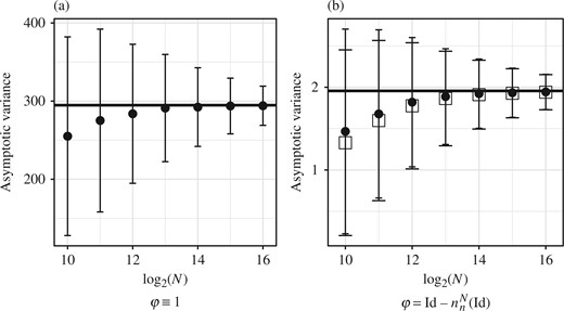
Estimated asymptotic variances |$NV_{n}^{N}(\varphi)$| (dots and error bars for the mean |$\pm$| one standard deviation from |$10^{4}$| replicates) against |$\log_{2}N$| for the linear Gaussian example. The horizontal lines correspond to the true asymptotic variances. The sample variances of |$\gamma_{n}^{N}(1)/\gamma_{n}(1)$| and |$\eta_{n}^{N}({\rm Id})$|⁠, scaled by |$N$|⁠, were close to their asymptotic variances. Corresponding results for the estimator of Chan & Lai (2013) are overlaid with boxes instead of dots and wider tick marks on the error bars.

Fig. 3.

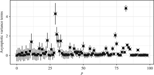
Plot of |$v_{p,n}^{N}(1)$| (dots and error bars for the mean |$\pm$| one standard deviation from |$10^{3}$| replicates) and |$v_{p,n}(1)$| (crosses) at each |$p\in\{0,\ldots,n\}$| for the linear Gaussian example, with |$N=10^{5}$|⁠.

We also compared a constant |$N$| particle filter, the asymptotically optimal particle filter where the asymptotically optimal allocation is computed exactly, and its approximation described in § 5.1 for different values of |$N$| using a Monte Carlo study with |$10^{4}$| replicates. We took |$g(N)=2/\log_{2}N$| in defining the approximation, and the results in Fig. 4(a) indicate that the approximation reduces the variance. The improvement is fairly modest for this particular model, and indeed the exact asymptotic variances associated with the constant |$N$| and asymptotically optimal particle filters differ by less than a factor of |$2$|⁠. In contrast, Fig. 4(b) shows that the improvement can be fairly dramatic in the presence of outlying observations; the improvement in variance there is by a factor of close to |$40$|⁠. Finally, we tested the adaptive particle filter described in § 5.2 using |$10^{4}$| replicates for each value of |$\delta$|⁠; results are displayed in Fig. 5, and indicate that the variances are close to their prescribed thresholds.

Fig. 4.

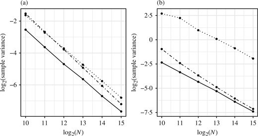
Logarithmic plots of sample variance for |$10^{4}$| replicates of |$\gamma_{n}^{N}(1)/\gamma_{n}(1)$| against |$N$| for the linear Gaussian example, using a constant |$N$| particle filter (dotted), the approximately asymptotically optimal particle filter (dot-dash), and the asymptotically optimal particle filter (solid). In panel (b), the observation sequence is |$y_{p}=0$| for |$p\in\{0,\ldots,99\}\setminus\{49\}$| and |$y_{49}=8$|⁠.

Fig. 5.

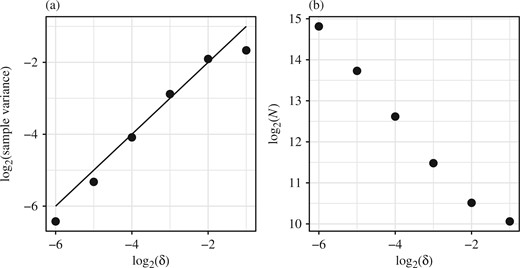
Logarithmic plots for the simple adaptive |$N$| particle filter estimates of |$\gamma_{n}(1)$| for the linear Gaussian example. Panel (a) plots the sample variance of |$\gamma_{n}^{N}(1)/\gamma_{n}(1)$| against |$\delta$|⁠, along with the straight line |$y=x$|⁠. Panel (b) plots |$N$| against |$\delta$|⁠, where |$N$| is the average number of particles used by the final particle filter.

6.2. Stochastic volatility hidden Markov model

A stochastic volatility model is defined by |$M_{0}(\cdot)=\mathcal{N}\{ \,\cdot\,;0,\sigma^{2}/(1-\rho^{2})\}$|⁠, |$M_{p}(x_{p-1},\cdot)=\mathcal{N}(\,\cdot\,;\rho x_{p-1},\sigma^{2})$| and |$G_{p}(x_{p})=\mathcal{N}\{y_{p};0,\beta^{2}\exp(x_{p})\}$|⁠. We used the pound/dollar daily exchange rates for 100 consecutive weekdays ending on 28th June 1985, a subset of the well-known dataset analysed in Harvey et al. (1994). Our results are obtained by choosing the parameters |$(\rho,\sigma,\beta)=(0{\cdot}95,0{\cdot}25,0{\cdot}5)$|⁠. We provide in the Supplementary Material plots of the accuracy of the estimate |$NV_{n}^{N}(\varphi)$| as |$N$| grows using |$10^{4}$| replicates for each value of |$N$|⁠; the asymptotic variances |$\sigma_{n}^{2}(1)$| and |$\sigma_{n}^{2}\{{\rm Id}-\eta_{n}({\rm Id})\}$| are estimated as being approximately |$347$| and |$1{\cdot}24$| respectively. In the Supplementary Material we plot the estimates of |$v_{p,n}(\varphi)$|⁠. We found modest improvement for the approximation of the asymptotically optimal particle filter, as one could infer from the estimated |$v_{p,n}(\varphi)$| and Lemma 5. For the simple adaptive |$N$| particle filter, results in the Supplementary Material indicate that the variances are close to their prescribed thresholds.

6.3. A sequential Monte Carlo sampler

We consider a sequential simulation problem, as described in § 2.3, with |$\mathsf{X=\mathbb{R}}$|⁠, |$\bar{\pi}_{0}(x)=\mathcal{N}(0,10^{2})$| and |$\bar{\pi}_{1}(x)=0{\cdot}3\mathcal{N}(x;-10,0{\cdot}1^{2})+0.7\mathcal{N}(x;10,0{\cdot}2^{2})$|⁠. The distribution |$\pi_{1}$| is bimodal with well-separated modes. With |$n=11$| and the sequence of tempering parameters

\[ \beta_{0:n}=(0,0{\cdot}0005,0{\cdot}001,0{\cdot}0025,0{\cdot}005,0{\cdot}01,0{\cdot}025,0{\cdot}05,0{\cdot}1,0{\cdot}25,0{\cdot}5,1), \]

we let each Markov kernel |$M_{p}$|⁠, |$p\in\{1,\ldots,n\}$|⁠, be an |$\eta_{p}$|-invariant random walk Metropolis kernel iterated |$k=10$| times with proposal variance |$\tau_{p}^{2}$|⁠, where |$\tau_{1:n}=(10,9,8,7,6,5,4,3,2,1,1)$|⁠.

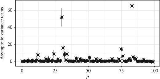
One striking difference between the estimates for this model and those for the hidden Markov models above is that the asymptotic variance |$\sigma_{n}^{2}\{{\rm Id}-\eta_{n}({\rm Id})\}\approx822$| is considerably larger than |$\sigma_{n}^{2}(1)\approx2{\cdot}1$|⁠; the variability of the estimates |$NV_{n}^{N}(\varphi)$| is shown in the Supplementary Material. Inspection of the estimates of |$v_{p,n}(\varphi)$| in Fig. 6 allows us to investigate both this difference and the dependence of |$v_{p,n}(\varphi)$| on |$k$| in greater detail.

Fig. 6.

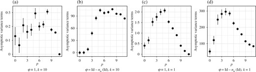
Plot of |$v_{p,n}^{N}(\varphi)$| (dots and error bars for the mean |$\pm$| one standard deviation) at each |$p\in\{0,\ldots,n\}$| with |$k=10$| iterations in (a) and (b) and with |$k=1$| iteration in (c) and (d) for each Markov kernel in the sequential Monte Carlo sampler example and |$N=10^{5}$|⁠.

Figure 6(a) and (b) show that while |$v_{p,n}(1)$| is small for all |$p$|⁠, the values of |$v_{p,n}\{{\rm Id}-\eta_{n}({\rm Id})\}$| are larger for large |$p$| than for small |$p$|⁠; this could be due to the inability of the Metropolis kernels |$(M_{q})_{q\geq p}$| to mix well due to the separation of the modes in |$(\eta_{q})_{q\geq p}$| when |$p$| is large. In Fig. 6(c) and (d), |$k=1$|⁠, i.e., each |$M_{p}$| consists of only a single iterate of a Metropolis kernel, and we see that the values of |$v_{p,n}(\varphi)$| associated with small |$p$| are much larger than when |$k=10$|⁠, indicating that the larger number of iterates does improve the asymptotic variance of the particle approximations. However, the effect on |$v_{p,n}(\varphi)$| is less pronounced for large |$p$|⁠. Results for the simple adaptive |$N$| particle filter approximating |$\eta_{n}({\rm Id})$| are provided in the Supplementary Material, which again show that the estimates are close to their prescribed thresholds.

7. Discussion

7.1. Alternatives to the bootstrap particle filter

In the hidden Markov model examples in § 6, we have constructed the Feynman–Kac measures taking |$M_{0},\ldots,M_{n}$| to be the initial distribution and transition probabilities of the latent process and defining |$G_{0},\ldots,G_{n}$| to incorporate the realized observations. This is only one, albeit important, way to construct particle approximations of |$\eta_{n}$|⁠, and the algorithm itself is usually referred to as the bootstrap particle filter. Alternative specifications of |$(M_{p},G_{p})_{0\leq p\leq n}$| lead to different Feynman–Kac models, as discussed in Del Moral (2004, § 2.4.2), and the variance estimators introduced here are applicable to these models as well.

One particular specification corresponds to the fully adapted auxiliary particle filter of Pitt & Shephard (1999), as discussed by Doucet & Johansen (2008). Specifically, we define |$\check{M}_{0}({\rm d}x_{0})=M_{0}({\rm d}x_{0})G_{0}(x_{0})/M_{0}(G_{0})$| and

\[ \check{M}_{p}(x_{p-1},{\rm d}x_{p})=\frac{M_{p}(x_{p-1},{\rm d}x_{p})G_{p}(x_{p})}{M_{p}(G_{p})(x_{p-1})},\qquad p\in[n], \]

and then |$\check{G}_{0}(x_{0})=M_{0}(G_{0})M_{1}(G_{1})(x_{0})$| and |$\check{G}{}_{p}(x_{p})=M_{p+1}(G_{p+1})(x_{p})$| for |$p\geq1$|⁠. If we denote by |$\check{\gamma}_{n}$| and |$\check{\eta}_{n}$| the Feynman–Kac measures associated with |$(\check{M}_{p},\check{G}_{p})_{0\leq p\leq n}$|⁠, we obtain |$\check{\gamma}_{n-1}(1)=\gamma_{n}(1)$|⁠. Moreover, the variance of |$\check{\gamma}_{n-1}^{N}(1)$| is often smaller than the variance of |$\gamma_{n}^{N}(1)$|⁠. In Fig. 7, we plot the corresponding |$\check{v}_{p,n-1}(1)$| and their approximations for the same linear Gaussian example as in § 6.1. Here, the asymptotic variance of |$\check{\gamma}_{n-1}^{N}(1)/\check{\gamma}_{n-1}(1)$| is 40|$\cdot$|679, more than seven times smaller than |$\sigma_{n}^{2}(1)$|⁠.

Fig. 7.

Plot of |$\check{v}_{p,n}^{N}(1)$| (dots and error bars for the mean |$\pm$| one standard deviation) and |$\check{v}_{p,n}(1)$| (crosses) at each |$p\in\{0,\ldots,n\}$| in the linear Gaussian example.

7.2. Estimators based on independent, identically distributed replicates

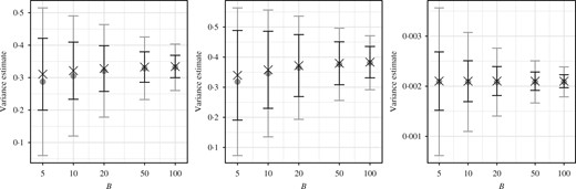
It is clearly possible to consistently estimate the variance of |$\gamma_{n}^{N}(\varphi)/\gamma_{n}(1)$| by using independent identically distributed replicates of |$\gamma_{n}^{N}$|⁠. Such estimates necessarily entail simulation of multiple particle filters. We now compare the accuracy of such estimates with those based on independent, identically distributed replicates of |$V_{n}^{N}(\varphi)$|⁠. For some |$\varphi\in\mathcal{L}(\mathcal{X})$| and |$B\in\mathbb{N}$|⁠, let |$\gamma_{n,i}^{N}(\varphi)$| and |$V_{n,i}^{N}(\varphi)$| be independent and identically distributed replicates for |$i\in[B]$|⁠, and define |$M=N^{-1}\sum_{i\in[B]}\gamma_{n,i}^{N}(1)$|⁠. A standard estimate of |${\rm var}\{ \gamma_{n}^{N}(\varphi)/\gamma_{n}(1)\}$| is obtained by calculating the sample variance of |$\{M^{-1}\gamma_{n,i}^{N}(\varphi)\::\:i\in[B]\}$|⁠. Noting the lack of bias of |$\gamma_{n}^{N}(1)^{2}V_{n}^{N}(\varphi)$|⁠, an alternative estimate of |${\rm var}\{ \gamma_{n}^{N}(\varphi)/\gamma_{n}(1)\}$| can be obtained as |$B^{-1}\sum_{i\in[B]}\{ M^{-1}\gamma_{n,i}^{N}(1)\} ^{2}V_{n,i}^{N}(\varphi)$|⁠. Both these estimates can be seen as ratios of simple Monte Carlo estimates of |${\rm var}\{ \gamma_{n}^{N}(\varphi)\}$| and |$\gamma_{n}(1)^{2}$|⁠, and are therefore consistent as |$B\rightarrow\infty$|⁠. We show in Fig. 8 a comparison between these estimates for the three models discussed in § 6 with |$N=10^{3}$| and |$\varphi\equiv1$|⁠, and we can see that the alternative estimate based on |$V_{n}^{N}(1)$| is empirically more accurate for these examples.

Fig. 8.

Plot of the standard estimate of |${\rm var}\{ \gamma_{n}^{N}(\varphi)/\gamma_{n}(1)\}$| (gray dots and error bars) and the alternative estimate using |$V_{n}^{N}(1)$| (black crosses and error bars) against |$B$| in (left to right) the examples of § 6.1–6.3.

7.3. Final remarks

The particular approximations developed here provide a natural way to estimate the terms appearing in the non-asymptotic second-moment expression (7). We have also provided the first generally applicable, consistent estimators of |$v_{p,n}(\varphi)$|⁠. The expression (7) does not apply to particle approximations with resampling schemes other than multinomial; one possible avenue of future research is to investigate these other settings. Whilst we have emphasized variances and asymptotic variances, the measures |$\mu_{b}$| also appear in expressions which describe propagation of chaos properties of the particle system. For instance, in the situation |$N_{p}\equiv N$|⁠, the asymptotic bias formula of Del Moral et al. (2007, p.7) can be expressed as

\[ NE\left\{ \eta_{n}^{N}(\varphi)-\eta_{n}(\varphi)\right\} \rightarrow-\sum_{p=0}^{n-1}\frac{\eta_{p}[Q_{p,n}(1)Q_{p,n}\{\varphi-\eta_{n}(\varphi)\}]}{\eta_{p}Q_{p,n}(1)^{2}}\equiv-\sum_{p=0}^{n-1}\frac{\mu_{e_{p}}[1\otimes\{\varphi-\eta_{n}(\varphi)\}]}{\gamma_{n}(1)^{2}}, \]

which can be consistently estimated using |$\mu_{e_{p}}^{N}$| and |$\gamma_{n}^{N}$|⁠. Finally, the technique used to prove Lemma 2 can be generalized to arbitrary positive integer moments of |$\gamma_{n}^{N}(\varphi)$|⁠.

In many applications, particularly in the context of hidden Markov models, particle filters are used to approximate conditional expectations with respect to updated Feynman–Kac measures. We define these, their approximations, and provide corresponding variance estimators in the Supplementary Material. Of some interest is the updated estimator |$\hat{\gamma}_{n-1}^{N}(1)=\gamma_{n}^{N}(1)$| whose variance estimator is |$\hat{V}_{n-1}^{N}(1)=V_{n-1}^{N}(G_{n-1})/\eta_{n-1}^{N}(G_{n-1})^{2}\neq V_{n}^{N}(1)$|⁠. In fact, |$V_{n}^{N}(1)$| is an unbiased, noisy approximation of |$\hat{V}_{n-1}^{N}(1)$|⁠, due to using |$E_{n}$| instead of |$G_{n-1}$| and |$\zeta_{n-1}$|⁠. However, empirical investigations indicate that the difference in variance is practically negligible.

Acknowledgement

This paper was first submitted when Anthony Lee was at the University of Warwick. He was partially supported by the Alan Turing Institute.

Supplementary material

Supplementary material available at Biometrika online includes algorithms for efficient computation of the variance estimators, results for estimators associated with updated Feynman–Kac measures, additional figures and proofs.

Appendix

 

Proof of Theorem 1.

Throughout the proof, |$\to$| denotes convergence in probability. For part (i), the fact |$\mu_{0_{n}}(\varphi^{\otimes2})=\gamma_{n}(\varphi)^{2}$| and Theorem 2 together give

\[ E\left\{ \gamma_{n}^{N}(1)^{2}V_{n}^{N}(\varphi)\right\} =E\left\{ \gamma_{n}^{N}(\varphi)^{2}-\mu_{0_{n}}^{N}(\varphi^{\otimes2})\right\} =E\left\{ \gamma_{n}^{N}(\varphi)^{2}\right\} -\gamma_{n}(\varphi)^{2}={\rm var}\left\{ \gamma_{n}^{N}(\varphi)\right\} \text{.} \]

For part (ii), combining the identity (12), |$\mu_{b}^{N}(\varphi^{\otimes2})\to\mu_{b}(\varphi^{\otimes2})$| by Theorem 2, and the fact that for any |$b\in B_{n}$| other than |$0_{n}$| and |$e_{0},\ldots,e_{n}$|⁠, |$\prod_{p=0}^{n}({1}/{N_{p}})^{b_{p}}(1-{1}/{N_{p}})^{1-b_{p}}$| is in |${O}(N^{-2})$|⁠, we obtain

\begin{equation} \gamma_{n}^{N}(\varphi)^{2}-\mu_{0_{n}}^{N}(\varphi^{\otimes2})=\left\{ \sum_{p=0}^{n}\frac{\mu_{e_{p}}^{N}(\varphi^{\otimes2})-\mu_{0_{n}}^{N}(\varphi^{\otimes2})}{\left\lceil c_{p}N\right\rceil }\right\} +{O}_{\rm p}(N^{-2})\text{.} \end{equation}

(A1)

Also noting that by Proposition 1 |$\gamma_{n}^{N}(1)^{2}\to\gamma_{n}(1)^{2}$| and that from (8) we have |$\gamma_{n}(1)^{2}v_{p,n}(\varphi)=\mu_{e_{p}}(\varphi^{\otimes2})-\mu_{0_{n}}(\varphi^{\otimes2})$| and again using |$\mu_{b}^{N}(\varphi^{\otimes2})\to\mu_{b}(\varphi^{\otimes2})$|⁠, we then have

\begin{equation} NV_{n}^{N}(\varphi)=\frac{N}{\gamma_{n}^{N}(1)^{2}}\left\{ \gamma_{n}^{N}(\varphi)^{2}-\mu_{0_{n}}^{N}(\varphi^{\otimes2})\right\} \to\sum_{p=0}^{n}\frac{v_{p,n}(\varphi)}{c_{p}}=\sigma_{n}^{2}(\varphi)\text{.} \end{equation}

(A2)

For part (iii), first note that by Theorem 2 and Proposition 1, for any |$b\in B_{n}$|⁠,

\begin{eqnarray*} \mu_{b}^{N}[\{\varphi-\eta_{n}^{N}(\varphi)\}^{\otimes2}] & = & \mu_{b}^{N}(\varphi^{\otimes2})-\eta_{n}^{N}(\varphi)\{\mu_{b}^{N}(\varphi\otimes1)+\mu_{b}^{N}(1\otimes\varphi)\}+\eta_{n}^{N}(\varphi)^{2}\mu_{b}^{N}(1^{\otimes2})\\ & \to & \mu_{b}[\{\varphi-\eta_{n}(\varphi)\}^{\otimes2}], \end{eqnarray*}

from which it follows that (A1) also holds with |$\varphi$| replaced by |$\varphi-\eta_{n}^{N}(\varphi)$|⁠, and similarly to (A2),

\begin{align*} NV_{n}^{N}\{\varphi-\eta_{n}^{N}(\varphi)\}\to\sum_{p=0}^{n}\frac{v_{p,n}\{\varphi-\eta_{n}(\varphi)\}}{c_{p}}=\sigma_{n}^{2}\left\{ \varphi-\eta_{n}(\varphi)\right\} \text{.}\\[-4pc] \end{align*}

□

 

Proof of Lemma 4.

For |$i\in[N_{n}]$| define |$B_{n-1}^{i}=A_{n-1}^{i}$| and |$B_{p-1}^{i}=A_{p-1}^{B_{p}^{i}}$| for |$p\in[n-1]$|⁠. Since in Algorithm 1, |$E_{p}^{i}=E_{p-1}^{A_{p-1}^{i}}$| for all |$p\in[n]$| and |$i\in[N_{p}]$|⁠, a simple inductive argument then shows that

\begin{equation} E_{n}^{i}=E_{p}^{B_{p}^{i}},\quad p\in\{0,\dots,n\},\,i\in[N_{n}]\text{.} \end{equation}

(A3)

We shall now prove |$(K^{1},K^{2})\in\mathcal{I}(0_{n})\Rightarrow E_{n}^{K_{n}^{1}}\neq E_{n}^{K_{n}^{2}}$|⁠. Recall from § 3.1 that when |$(K^{1},K^{2})\in\mathcal{I}(0_{n})$|⁠, we have |$A_{p-1}^{K_{p}^{1}}=K_{p-1}^{1}\neq K_{p-1}^{2}=A_{p-1}^{K_{p}^{2}}$| for all |$p\in[n]$|⁠, hence |$B_{0}^{K_{n}^{1}}=K_{0}^{1}\neq K_{0}^{2}=B_{0}^{K_{n}^{2}}$|⁠. Applying (A3) with |$p=0$| and using the fact that in Algorithm 1, |$E_{0}^{i}=i$| for all |$i\in[N_{n}]$|⁠, we have |$E_{n}^{i}=E_{0}^{B_{0}^{i}}=B_{0}^{i}$|⁠, hence |$E_{n}^{K_{n}^{1}}=B_{0}^{K_{n}^{1}}\neq B_{0}^{K_{n}^{2}}=E_{n}^{K_{n}^{2}}$| as required. It remains to prove |$(K^{1},K^{2})\notin\mathcal{I}(0_{n})\Rightarrow E_{n}^{K_{n}^{1}}=E_{n}^{K_{n}^{2}}$|⁠. Assuming |$(K^{1},K^{2})\notin\mathcal{I}(0_{n})$|⁠, consider |$\tau=\mathrm{max}\{p:K_{p}^{1}=K_{p}^{2}\}$|⁠. If |$\tau=n$| then clearly |$E_{n}^{K_{n}^{1}}=E_{n}^{K_{n}^{2}}$|⁠, so suppose |$\tau<n$|⁠. It follows from § 3.1 that |$B_{\tau}^{K_{n}^{1}}=K_{\tau}^{1}=K_{\tau}^{2}=B_{\tau}^{K_{n}^{2}}$|⁠, so taking |$p=\tau$| and |$i=K_{n}^{1},K_{n}^{2}$| in (A3) gives |$E_{n}^{K_{n}^{1}}=E_{n}^{K_{n}^{2}}$|⁠. □

 

Proof of Theorem 3.

For part (i), Theorem 2 gives

\[ E\left\{ \gamma_{n}^{N}(1)^{2}v_{p,n}^{N}(\varphi)\right\} =E\left\{ \mu_{e_{p}}^{N}(\varphi^{\otimes2})-\mu_{0_{n}}^{N}(\varphi^{\otimes2})\right\} =\mu_{e_{p}}(\varphi^{\otimes2})-\mu_{0_{n}}(\varphi^{\otimes2})=\gamma_{n}(1)^{2}v_{p,n}(\varphi)\text{.} \]

For the remainder of the proof, |$\to$| denotes convergence in probability. For part (ii), |$\mu_{e_{p}}^{N}(\varphi^{\otimes2})-\mu_{0_{n}}^{N}(\varphi^{\otimes2})\to\gamma_{n}(1)^{2}v_{p,n}(\varphi)$| by Theorem 2, and |$\gamma_{n}^{N}(1)^{2}\to\gamma_{n}(1)^{2}$| by Proposition 1, so |$v_{p,n}^{N}(\varphi)=\{\mu_{e_{p}}^{N}(\varphi^{\otimes2})-\mu_{0_{n}}^{N}(\varphi^{\otimes2})\}/\gamma_{n}^{N}(1)^{2}\to v_{p,n}(\varphi)$|⁠; as in the proof of Theorem 1, |$\mu_{b}^{N}[\{\varphi-\eta_{n}^{N}(\varphi)\}^{\otimes2}]\to\mu_{b}[\{\varphi-\eta_{n}(\varphi)\}^{\otimes2}]$| gives |$v_{p,n}^{N}\{\varphi-\eta_{n}^{N}(\varphi)\}\to v_{p,n}\{\varphi-\eta_{n}(\varphi)\}$|⁠. Part (iii) follows from (i) and (ii). □

Author notes