A semiparametric extension of the stochastic block model for longitudinal networks

Summary

We propose an extension of the stochastic block model for recurrent interaction events in continuous time, where every individual belongs to a latent group and conditional interactions between two individuals follow an inhomogeneous Poisson process with intensity driven by the individuals’ latent groups. We show that the model is identifiable and estimate it with a semiparametric variational expectation-maximization algorithm. We develop two versions of the method, one using a nonparametric histogram approach with an adaptive choice of the partition size, and the other using kernel intensity estimators. We select the number of latent groups by an integrated classification likelihood criterion. We demonstrate the performance of our procedure on synthetic experiments, analyse two datasets to illustrate the utility of our approach, and comment on competing methods.

1. Introduction

Over the past few years there has been increasing interest in modelling dynamic interactions between individuals. Continuous-time information on interactions is often available, for example as email exchanges between employees in a company (Klimt & Yang, 2004) or as face-to-face contacts between individuals measured by sensors (Stehlé et al., 2011), but most models are based on discrete time. Commonly, data are aggregated on predefined time intervals to obtain a sequence of snapshots of random graphs. Apart from the loss of information due to aggregation, the choice of the time intervals has a direct impact on the results, so developing continuous-time models is important. These are called longitudinal networks, interaction event data, link streams or temporal networks.

There are many statistical methods for longitudinal networks, especially in social science; see Holme (2015) for a review. It is natural to model temporal event data by stochastic point processes. An important line of research involves continuous-time Markov processes, with seminal works on dyad-independent models (Wasserman, 1980a, b) or so-called stochastic actor-oriented models (Snijders & van Duijn, 1997; Snijders et al., 2010). In these works, interactions last for some time. Here, in contrast, we focus on instantaneous interactions identified by time-points, and we model dependencies between interactions of pairs of individuals.

The analysis of event data is well established (Andersen et al., 1993). Generally, the numbers of interactions between all pairs |$(i,j)$| of individuals up to time |$t$| are modelled by a multivariate counting process |$N(t)=\{N_{i,j}(t)\}_{(i,j)}$|⁠. Butts (2008) considered time-stamped interactions marked by a label representing a behavioural event. His model is an instance of Cox’s multiplicative hazard model with time-dependent covariates and constant baseline function. In the same vein, Vu et al. (2011) proposed regression-based modelling of the intensity of nonrecurrent interaction events. They considered two different frameworks: Cox’s multiplicative and Aalen’s additive hazard rates. Perry & Wolfe (2013) proposed another variant of Cox’s multiplicative intensity model for recurrent interaction events, where the baseline function is specific to each individual. In the above-mentioned works, a set of statistics chosen by the user may modulate the interactions. As in any regression framework, the choice of these statistics raises some issues: increasing their number may lead to a high-dimensional problem, and interpretation of the results could be blurred by their possible correlations.

The approaches of Butts (2008), Vu et al. (2011), Perry & Wolfe (2013) and others are based on conditional Poisson processes characterized by random intensities, also known as doubly stochastic Poisson processes or Cox processes. An example of a conditional Poisson process is the Hawkes process (Hawkes, 1971), which is a collection of point processes with some background rate, where each event adds a nonnegative impulse to the intensity of all the other processes. Blundell et al. (2012) extended the infinite relational model by introducing reciprocating Hawkes processes to parameterize edges and make all events codependent over time. Cho et al. (2014) developed a model for spatial-temporal networks with missing information, based on Hawkes processes for temporal dynamics combined with a Gaussian mixture for the spatial dynamics. Similarly, Linderman & Adams (2014) combined temporal Hawkes processes with latent distance models for implicit networks. Models associating point processes with single nodes rather than pairs also exist; see Fox et al. (2016) and the references therein.

Clustering individuals based on interaction data is a well-established way to account for the intrinsic heterogeneity and to summarize information. For discrete-time sequences of graphs, recent works have proposed generalizations of the stochastic block model to a dynamic context (Yang et al., 2011; Xu & Hero, 2014; Corneli et al., 2016; Matias & Miele, 2017). Stochastic block models posit that all individuals belong to one of finitely many groups, and given these groups all pairs of interactions are independent. Stochastic block models induce more general clusterings than do community detection algorithms. Indeed, clusters are not necessarily characterized by intense within-group interaction and low interaction frequency with other groups. Another attempt to use stochastic block models for interaction events appears in DuBois et al. (2013), which generalizes the approach of Butts (2008) by adding discrete latent variables for the individuals.

We introduce a semiparametric stochastic block model for recurrent interaction events in continuous time, which we refer to as the Poisson process stochastic block model. Interactions are modelled by conditional inhomogeneous Poisson processes, whose intensities depend only on the latent groups of the interacting individuals. We do not rely on a parametric model where intensities are modulated by predefined network statistics; they are modelled and estimated in a nonparametric way. The model parameters are shown to be identifiable. Our estimation and clustering approach is a semiparametric version of the variational expectation-maximization algorithm, where the maximization step is replaced by nonparametric estimators of the intensities. Semiparametric generalizations of the classical expectation-maximization algorithm have been proposed in many different contexts; see Böhning (1995), Bordes et al. (2007) and Robin et al. (2007) for semiparametric mixtures or Dannemann (2012) for a semiparametric hidden Markov model. However, we are not aware of other attempts to incorporate nonparametric estimation in a variational approximation algorithm. We propose two different estimators of the nonparametric part of the model: a histogram approach using Reynaud-Bouret (2006), where the partition size is adaptively chosen, and a kernel estimator based on Ramlau-Hansen (1983). With the histogram approach, an integrated classification likelihood criterion is proposed to select the number of latent groups. Synthetic experiments and analysis of two datasets illustrate the strengths and weaknesses of our approach. The code is available in the R (R Development Core Team, 2018) package ppsbm.

2. A semiparametric Poisson process stochastic block model

2.1. Model

We consider pairwise interactions of |$n$| individuals during some time interval |$[0,T]$|⁠. For notational convenience we restrict our attention to directed interactions without self-interactions. The undirected case and self-interactions are handled similarly. The set of all pairs of individuals, i.e., the set of all possible dyads in the graph, is denoted by

$$ \mathcal R=\{(i,j) : i,j=1,\ldots,n;\: i\neq j\}, $$

which has cardinality |$r=n(n-1)$|⁠. We observe the interactions during the time interval |$[0,T]$|⁠, that is,

$$ \mathcal O=\{(t_m,i_m,j_m): m=1,\ldots,M\}, $$

where |$(t_m,i_m,j_m)\in[0,T]\times \mathcal R$| corresponds to the event that a directed interaction from the |$i_m$|th individual to the |$j_m$|th individual occurs at time |$t_m$|⁠. The random total number of events is |$M$|⁠. We assume that |$0<t_1<\dots< t_M<T$|⁠, i.e., there is at most one event at a time.

Every individual is assumed to belong to one of |$Q$| groups, and the relation between two individuals, i.e., how they interact with one another, is driven by their group membership. Let |$Z_1,\ldots,Z_n$| be independent and identically distributed latent random variables taking values in |$\{1,\ldots,Q\}$| with nonzero probabilities |${\mathrm{pr}}(Z_1=q) =\pi_q$||$(q=1,\ldots,Q)$|⁠. For the moment, |$Q$| is treated as fixed and known. When no confusion is likely to occur, we also use the notation |$Z_i=(Z^{i,1},\ldots,Z^{i,Q})$| where |$Z^{i,q}\in\{0,1\}$| such that |$Z_i$| has multinomial distribution |$\mathcal M(1,\pi)$| with |$\pi=(\pi_1,\ldots,\pi_Q)$|⁠.

For every pair |$(i,j)\in\mathcal R$|⁠, the interactions from individual |$i$| to |$j$| conditional on the latent groups |$Z_1,\ldots,Z_n$| are modelled by a conditional inhomogeneous Poisson process |$N_{i,\,j}(\cdot)$| on |$[0,T]$| with intensity depending only on |$Z_i$| and |$Z_j$|⁠. For |$q, l=1,\ldots, Q$| and |$(i,j)\in\mathcal R$|⁠, the conditional intensity of |$N_{i,j}(\cdot)$| given |$Z_i=q$| and |$Z_j=l$| is |$\alpha^{(q,l)}(\cdot)$|⁠, with corresponding cumulative intensity

$$ A^{(q,l)} (t)= \int_0^t \alpha^{(q,l)}(u)\,{\mathrm{d}} u \quad (0\le t \le T)\text{.} $$

The set of observations |$\mathcal O$| is a realization of the multivariate counting process |$\{N_{i,j}(\cdot)\}_{(i,j)\in \mathcal{R}}$| with conditional intensity process |$\{\alpha^{(Z_i,Z_j)}(\cdot)\}_{(i,j)\in \mathcal{R}}$|⁠. The process |$N_{i,j}$| has intensity |$\sum_{q=1}^Q\sum_{l=1}^Q\pi_q\pi_l \alpha^{(q,l)}$|⁠. We let |$\theta =(\pi,\alpha)$| denote the infinite-dimensional parameter of our model and write |${\mathrm{pr}_\theta}$| for the Poisson process stochastic block model distribution of the multivariate counting process |$\{N_{i,j}(\cdot)\}_{(i,j)\in \mathcal{R}}$|⁠. An extension that accounts for sparse interaction processes is given in the Supplementary Material.

2.2. Identifiability

Identifiability of the parameter |$\theta$| corresponds to injectivity of |$\theta \mapsto {\mathrm{pr}_\theta}$| and may be obtained, if at all, up to label switching, as defined below. We let |$\mathfrak{S}_Q$| denote the set of permutations of |$\{1,\ldots, Q\}$|⁠.

 

Definition 1.

The parameter |$\theta=(\pi, \alpha)$| of a Poisson process stochastic block model is identifiable on |$[0,T]$| up to label switching if for all |$\theta$| and |$\tilde\theta$| such that |${\mathrm{pr}_\theta} = \mathrm{pr}_{\tilde \theta}$| there exists a permutation |$\sigma \in \mathfrak{S}_Q$| such that |$\pi_q =\tilde \pi_{\sigma(q)}$| and |$\alpha^{(q,l)} = \tilde \alpha^{(\sigma(q),\sigma(l))}$| almost everywhere on |$[0,T]$| for |$q, l=1,\ldots, Q$|.

Identifiability up to label switching is ensured in the very general setting where the intensities |$\alpha^{(q,l)}$| are not equal almost everywhere.

 

Assumption 1.

The set of intensities |$\{\alpha^{(q,l)}\}_{q, l=1,\ldots, Q}$| contains exactly |$Q^2$| distinct functions in the directed case, and |$Q(Q+1)/2$| in the undirected case.

 

Proposition 1.

Under Assumption 1, the parameter |$\theta=(\pi,\alpha)$| is identifiable on |$[0,T]$| up to label switching from the Poisson process stochastic block model distribution |${\mathrm{pr}_\theta}$|⁠, as soon as |$n\ge 3$|.

Assumption 1 is similar to the hypothesis from Theorem 12 in Allman et al. (2011), which, to our knowledge, is the only identifiability result for weighted stochastic block models. The question of whether the necessary condition that any two rows or any two columns of the parameter matrix |$\alpha$| are distinct is also a sufficient condition for identifiability remains open even in the simpler binary case. In the binary stochastic block model, Allman et al. (2009, 2011) established generic identifiability, which means identifiability except on a subset of parameters with Lebesgue measure zero, without specifying this subset. For the directed and binary stochastic block model, Celisse et al. (2012) established identifiability under the assumption that the product vector |$\alpha \pi$|⁠, or |$\pi^{{\rm T}} \alpha$|⁠, has distinct coordinates. This condition is slightly stronger than requiring any two rows of the parameter matrix to be distinct. Another identifiability result appears in Bickel et al. (2011) for some specific block models. These last two approaches are specific to the binary set-up and cannot be generalized to the continuous case.

Proposition 1 does not cover the undirected affiliation case, where only two intensities |$\alpha^{\mathrm{in}}$| and |$\alpha^{\mathrm{out}}$| are considered such that |$\alpha^{(q,q)}=\alpha^\mathrm{in}$| and |$\alpha^{(q,l)}=\alpha^\mathrm{out}$||$(q,l=1,\ldots, Q;\, q\neq l)$|⁠.

 

Proposition 2.

If the intensities |$\alpha^\mathrm{in}$| and |$\alpha^\mathrm{out}$| are distinct functions on |$[0,T]$|⁠, then both |$\alpha^\mathrm{in}$| and |$\alpha^\mathrm{out}$| are identifiable on |$[0,T]$| from the undirected affiliation Poisson process stochastic block model distribution |${\mathrm{pr}_\theta}$| when |$n\ge 3$|⁠. Moreover, for |$n\ge \max(Q, 3)$|⁠, the proportions |$\pi_1,\ldots, \pi_Q$| are also identifiable up to a permutation.

2.3. Additional notation

We introduce some quantities that will be relevant below. Let

\begin{align} Y^{(q,l)}_{\mathcal Z} &= \sum_{(i,j)\in\mathcal R}Z^{i,q}Z^{j,l} \quad (q, l=1,\ldots, Q), \label{Yql}\\ \end{align}

(1)

\begin{align} N_{{\mathcal{Z}}}^{(q,l)} &=\sum_{(i,j)\in\mathcal R} Z^{i,q}Z^{j,l} N_{i,j} \quad (q, l=1,\ldots, Q), \label{eq:N_Z}\\ \end{align}

(2)

\begin{align} Z_{m}^{(q,l)} &= Z^{i_m,q}Z^{j_m,l} \quad (q, l=1,\ldots, Q;\: m=1,\ldots,M)\text{.} \label{eq:Zmql} \end{align}

(3)

These are, respectively, the latent number of dyads |$(i,j)\in \mathcal{R}$| with latent groups |$(q,l)$|⁠, the latent counting process of interactions between individuals in groups |$(q,l)$|⁠, and the latent binary indicator of observation |$(t_m,i_m,j_m)$| belonging to groups |$(q,l)$|⁠. As these quantities are unobserved, our work relies on proxies based on approximations of the latent group variables |$Z^{i,q}$|⁠. Write

\begin{equation} \label{eq:tau_class} \mathcal T=\left\{\tau=(\tau^{i,q})_{i=1,\ldots,n; \,q=1,\ldots,Q} : \tau^{i,q}\ge 0, \; \sum_{q=1}^Q\tau^{i,q}=1 \; (i=1,\ldots,n;\, q=1,\ldots,Q) \right\}\!\text{.} \end{equation}

(4)

While the variables |$Z^{i,q}$| are indicators, their counterparts |$\tau^{i,q}$| are weights representing the probability that node |$i$| belongs to group |$q$|⁠. Now, for every |$\tau\in\mathcal T$|⁠, replacing all latent variables |$Z^{i,q}$| in (1)–(3) by |$\tau^{i,q}$|⁠, we define |$Y^{(q,l)}$|⁠, |$N^{(q,l)}$| and |$\tau_{m}^{(q,l)}$|⁠, which are estimators of |$Y^{(q,l)}_{\mathcal Z}$|⁠, |$N_{{\mathcal{Z}}}^{(q,l)}$| and |$Z_{m}^{(q,l)}$|⁠, respectively.

3. Semiparametric estimation procedure

3.1. A variational semiparametric expectation-maximization algorithm

The complete-data likelihood of observations |$\mathcal O$| and latent variables |$\mathcal Z=(Z_1,\ldots,Z_n)$| is

\[ \mathcal L (\mathcal O,\mathcal Z \mid \theta) =\exp\!\left\{-\!\sum_{(i,j)\in\mathcal R} A^{(Z_i,Z_j)}(T) \right\}\prod_{m=1}^M\alpha^{(Z_{i_m},Z_{j_m})}(t_m) \prod_{i=1}^n\prod_{q=1}^Q\pi_q^{Z^{i,q}}\text{.} \]

The likelihood of the observed data |$\mathcal L(\mathcal O\mid\theta)$| is obtained by summing the above over the set of all possible configurations of the latent variables |$\mathcal Z$|⁠. This set is huge, so the likelihood |$\mathcal L(\mathcal O\mid\theta)$| is intractable for direct maximization. Hence, an expectation-maximization algorithm (Dempster et al., 1977) is used. Two issues arise in our model. First, as already observed for the standard stochastic block model (Daudin et al., 2008), the E-step requires computation of the conditional distribution of |$\mathcal Z$| given the observations |$\mathcal O$|⁠, which is intractable. Therefore, we use a variational approximation (Jordan et al., 1999) of the latent variables’ conditional distribution to perform the E-step. See Matias & Robin (2014) on variational approximations in stochastic block models for more details. Second, part of our parameter is infinite-dimensional, so the M-step is partially replaced by a nonparametric estimation procedure.

3.2. Variational E-step

The standard E-step consists of computing the expectation of the complete-data loglikelihood given the observations at some current parameter value |$\theta$|⁠. This requires knowledge of the conditional distribution of the latent variables |${\mathrm{pr}}_\theta(\mathcal Z\mid\mathcal O)$|⁠, which is not tractable because the |$Z_i$| are not conditionally independent. Hence we use a variational approximation of |${\mathrm{pr}}_\theta(\mathcal Z\mid\mathcal O)$| by a simpler distribution. Using the class of parameters |$\mathcal{T}$| defined in (4), we consider the family of factorized distributions on |$\mathcal Z$| given |$\mathcal O$|⁠, defined as

\begin{align*} {\mathrm{pr}}_\tau\{\mathcal Z=(q_1,\ldots,q_n)\mid\mathcal O\} &=\prod_{i=1}^n{\mathrm{pr}}_\tau(Z_i=q_i\mid\mathcal O) =\prod_{i=1}^n \tau^{i,q_i}, \quad (q_1,\ldots,q_n) \in\{1,\ldots,Q\}^n, \end{align*}

with corresponding expectation |$E_\tau(\cdot\mid\mathcal O)$|⁠. Writing |${\small{\text{KL}}}(\cdot \| \cdot)$| for the Kullback–Leibler divergence, we search for the parameter |$\hat \tau\in\mathcal T$| that yields the best approximation |${\mathrm{pr}}_\tau(\cdot\mid\mathcal O)$| of |${\mathrm{pr}}_\theta(\cdot\mid\mathcal O)$| through

\begin{align}\label{eq:hat_tau} \hat\tau = \mathop{\arg\min}_{\tau\in\mathcal T}\,\,{{\small{\text{KL}}}\{{ {\mathrm{pr}}_\tau(\cdot\mid \mathcal{O}) } \,\|\, { {\mathrm{pr}}_{\theta}(\cdot\mid \mathcal{O}) }\}} \text{.} \end{align}

(5)

Let |$\mathcal{H}(\cdot)$| be the entropy of a distribution. It can be seen that |$\hat\tau$| maximizes with respect to |$\tau$| the quantity

\begin{align*} J(\theta,\tau) & = E_\tau\{ \log\mathcal L(\mathcal O,\mathcal Z\mid\theta)\mid\mathcal O\} +\mathcal{H}\{{\mathrm{pr}}_\tau(\cdot\mid \mathcal{O})\} \\ &= -\sum_{q=1}^Q\sum_{l=1}^Q Y^{(q,l)} A^{(q,l)}(T) + \sum_{q=1}^Q\sum_{l=1}^Q \sum_{m=1}^M\tau_{m}^{(q,l)} \log\bigl\{ \alpha^{(q,l)}(t_m)\bigr\}\\ & \quad + \sum_{i=1}^n\sum_{q=1}^Q{\tau^{i,q}}\log \left(\frac{\pi_q}{\tau^{i,q}} \right)\!\text{.} \end{align*}

The solution |$\hat \tau$| satisfies a fixed-point equation, and in practice is found by successively updating the variational parameters |$\tau^{i,q}$| via (6) until convergence.

 

Proposition 3.

The solution |$\hat \tau$| to the minimization problem (5) satisfies the fixed-point equation

\begin{equation} \label{eq_vstep_pi_q_fixed_point} \hat \tau^{i,q}\propto \pi_q \exp\{D_{iq}(\hat \tau, \alpha)\} \quad (i=1,\ldots,n;\: q=1,\ldots,Q), \end{equation}

(6)

where, with |${\rm 1}\kern-0.24em{\rm I}_A$| denoting the indicator function of set |$A$|,

\begin{align*} D_{iq}(\tau,\alpha)& = -\sum_{l=1}^Q \sum_{\substack{j=1\\ j\neq i}}^n \tau^{j,l} \bigl\{A^{(q,l)}(T)+A^{(l,q)}(T)\bigr\} \\[-2pt] &\quad+\sum_{l=1}^Q\sum_{m=1}^M \Big[ {\rm 1}\kern-0.24em{\rm I}_{\{i_m=i\}}\tau^{j_m,l} \log\bigl\{\alpha^{(q,l)}(t_m)\bigr\}+{\rm 1}\kern-0.24em{\rm I}_{\{j_m=i\}}\tau^{i_m,l}\log\bigl\{\alpha^{(l,q)}(t_m)\bigr\} \Big]\text{.} \end{align*}

3.3. Nonparametric M-step: general description

In a parametric context the M-step consists in the maximization of |$J(\theta,\tau)$| with respect to |$\theta=(\pi,\alpha)$|⁠. Considering only the finite-dimensional part, |$\pi$|⁠, of the parameter, the maximizer |$\hat \pi$| is

\begin{equation}\label{eq_mstep_pi_q} \hat \pi_q=\frac{\sum_{i=1}^n\tau^{i,q}}{\sum_{q=1}^Q\sum_{i=1}^n\tau^{i,q}} =\frac1n{\sum_{i=1}^n\tau^{i,q}} \quad (q=1,\ldots,Q)\text{.} \end{equation}

(7)

Concerning the infinite-dimensional parameter, |$\alpha$|⁠, we replace the maximization of |$J(\pi,\alpha,\tau)$| with respect to |$\alpha$| by a nonparametric estimation step. If the process |$N_{{\mathcal{Z}}}^{(q,l)}$| defined by (2) was observed, the estimation of |$\alpha^{(q,l)}$| would be straightforward. Now the criterion |$J$| depends on |$\alpha$| through |$E_\tau \{\log \mathcal L(\mathcal O,\mathcal Z \mid \theta) \mid \mathcal O \}$|⁠, which corresponds to the loglikelihood in a set-up where we observe the weighted cumulative process |$N^{(q,l)}$|⁠; see § 2.3. Intensities may be estimated easily in this direct observation set-up. We develop two different approaches to updating |$\alpha$|⁠: a histogram method and a kernel method.

3.4. Histogram-based M-step

In this part the intensities |$\alpha^{(q,l)}$| are estimated by piecewise-constant functions and we propose a data-driven choice of the partition of the time interval |$[0,T]$|⁠. The procedure is based on a least-squares penalized criterion, following Reynaud-Bouret (2006). Here |$(q,l)$| is fixed, and for reasons of computational efficiency we focus on regular dyadic partitions that form embedded sets of partitions.

For some given |$d_{\max}$|⁠, consider all regular dyadic partitions of |$[0,T]$| into |$2^d$| intervals,

\[ \mathcal{E}_d = \left\{ \mathcal I_{k} =\left[(k-1)\frac T {2^d} ,\, k \frac T{2^d} \right) : k =1,\ldots, 2^d\right\} \quad (d= 0,\ldots,d_{\max})\text{.} \]

For any interval |$\mathcal I$| included in |$[0,T]$|⁠, the estimated mean number of observed interactions |$(t_m,i_m,j_m)$| between individuals with latent groups |$(q,l)$| occurring in |$\mathcal I$| is

\begin{align*} N^{(q,l)}(\mathcal I)= \int_{\mathcal I} {\mathrm{d}} N^{(q,l)}(s) = \sum_{m=1}^M\tau^{i_m,q}\tau^{j_m,l}{\rm 1}\kern-0.24em{\rm I}_{\mathcal I}(t_m)\text{.} \end{align*}

The total number of dyads |$r$| is an upper bound for |$Y^{(q,l)}$|⁠, so we define a least-squares contrast relative to the counting process |$N^{(q,l)}$| for all |$f \in {L}^2([0,T],{\mathrm{d}} t)$| by

\begin{equation*} \gamma^{(q,l)}(f)=-\frac{2}{r} \int_0^T f(t) \,{\mathrm{d}} N^{(q,l)}(t) +\frac{Y^{(q,l)}}{r} \int_0^T f^2(t) \,{\mathrm{d}} t\text{.} \end{equation*}

The projection estimator of |$\alpha^{(q,l)}$| onto the set |$S_d$| of piecewise-constant functions on |$\mathcal{E}_d$| is

\begin{equation*} \hat{\alpha}_d ^{(q,l)}=\mathop{\arg\min}_{f \in S_d} \gamma^{(q,l)}(\hskip 2.3ptf)= \frac1{Y^{(q,l)}} \sum_{\mathcal I\in \mathcal{E}_d}\frac{N^{(q,l)}(\mathcal I)}{| \mathcal I| }{\rm 1}\kern-0.24em{\rm I}_{\mathcal I}(\cdot), \end{equation*}

where |$|\mathcal I|$| is the length of interval |$\mathcal I$|⁠, here equal to |$T2^{-d}$|⁠. Adaptive estimation consists in choosing the best estimator from the collection |$\{ \hat{\alpha}_d^{(q,l)} : d=0,\ldots, d_{\max} \}$| using a penalized least-squares criterion

\begin{equation*} \text{crit}^{(q,l)}(d)=\gamma^{(q,l)}(\hat{\alpha}_d^{(q,l)})+\text{pen}^{(q,l)}(d), \end{equation*}

for some penalty function |$\text{pen}^{(q,l)} : \{0,\ldots ,d_{\max}\}\rightarrow \mathbb{R}^{+}$| that penalizes large partitions. We choose the penalty function to be

\begin{equation*} \text{pen}^{(q,l)}(d)=\frac{2^{d+1}}{r} C , \quad C=\frac{ 2^{d_{\max}}}{T Y^{(q,l)}} \sup_{\mathcal I\in \mathcal{E}_{d_{\max}}} N^{(q,l)} (\mathcal I)\text{.} \end{equation*}

Finally, the penalized least-squares criterion simplifies to

\begin{equation*} {\hat{d}}^{(q,l)} = \mathop{\arg\min}_{ d =0,\ldots, d_{\max}} 2^d\left\{-\!\! \sum_{\mathcal I\in \mathcal{E}_d}N^{(q,l)}(\mathcal I)^2 + 2^{d_{\max} +1} \sup_{\mathcal I'\in \mathcal{E}_{d_{\max}}} N^{(q,l)} (\mathcal I') \right\}\!\text{.} \end{equation*}

The selected partition size |$\hat d=\hat d^{(q,l)}$| may be specific to the groups |$(q,l)$|⁠. Finally, the adaptive estimator of intensity |$\alpha^{(q,l)}$| is

\begin{equation} \hat {\alpha}^{(q,l)}_{\text{hist}} (t) = \hat \alpha_{\hat d}^{(q,l)}(t) =\frac{2^{\hat d }}{T Y^{(q,l)}} \sum_{\mathcal I\in \mathcal{E}_{\hat d}}N^{(q,l)} (\mathcal I) {\rm 1}\kern-0.24em{\rm I}_{\mathcal I }(t) \quad (0\leqslant t\leqslant T ; \: q,l=1,\ldots,Q)\text{.} \label{eq:mstep_histo} \end{equation}

(8)

Reynaud-Bouret (2006) developed her approach for the Aalen multiplicative intensity model, which is slightly different from our context. Moreover, our set-up does not satisfy the assumptions of Theorem 1 in Reynaud-Bouret (2006) as we have recurrent events, so the number of jumps of the processes |$N_{i,j}$| is not bounded by a known value. Nevertheless, in our simulations this procedure correctly estimates the intensities |$\alpha^{(q,l)}$|⁠; see § 4. See Baraud & Birgé (2009) for a theoretical study of an adaptive nonparametric estimation method for the intensity of a Poisson process. Reynaud-Bouret (2006) also studied other penalized least-squares estimators which could be used here.

3.5. Kernel-based M-step

Kernel methods are well suited to the estimation of smooth functions. If the variational parameters |$\tau^{i,q}$| are good approximations of the latent variables |$Z^{i,q}$|⁠, then the intensity of |$N^{(q,l)}$| is approximately |$Y^{(q,l)}\alpha^{(q,l)}$|⁠, where |$Y^{(q,l)}$| is the variational mean number of dyads with latent groups |$(q,l)$|⁠. Following Ramlau-Hansen (1983) and considering a nonnegative kernel function |$K$| with support within |$[-1,1]$| together with some bandwidth |$b>0$|⁠, the intensity |$\alpha^{(q,l)}$| is estimated by

\begin{align}\label{eq_mstep__kernel_lamb_ql} \hat{\alpha}_{\text{ker}}^{(q,l)}(t) &=\frac{1}{b Y^{(q,l)} } \int_0^T K\left(\frac{t-u}{b}\right){\mathrm{d}} N^{(q,l)}(u) =\frac{1}{b Y^{(q,l)}} \sum_{m=1}^M\tau_{m}^{(q,l)} K\left(\frac{t-t_m}{b} \right) \end{align}

(9)

if |$Y^{(q,l)}>0$| and |$\hat{\alpha}_{\text{ker}}^{(q,l)}(t)=0$| otherwise, where |$\tau_{m}^{(q,l)}$| is defined in § 2.3.

The bandwidth |$b$| could be chosen adaptively from the data following the procedure proposed by Grégoire (1993). Kernel methods are not always suitable for inferring a function on a bounded interval, as boundary effects may degrade their quality. However, it is beyond the scope of this work to investigate refinements of this kind.

3.6. Semiparametric variational expectation-maximization algorithm

The implementation of the algorithm raises two issues: convergence and initialization. As our algorithm is iterative, one has to test for convergence. A stopping criterion can be defined based on criterion |$J(\theta,\tau)$|⁠. Concerning initialization, the algorithm is run several times with different starting values, which are chosen by some |$k$|-means method combined with perturbation techniques; see the Supplementary Material. Algorithm 1 provides a description of the procedure.

 

Algorithm 1.

Semiparametric variational expectation-maximization algorithm.

|$\quad$|Set |$s=0$|

|$\quad$|Initialize |$\tau^{[0]}$|

|$\quad$|While convergence is not attained, do

|$\qquad$||$\quad$|Update |$\pi^{[s+1]}$| via (7) with |$\tau=\tau^{[s]}$|

|$\qquad$||$\quad$|Update |$\alpha^{[s+1]}$| via (8) for histogram method or (9) for kernel method with |$\tau=\tau^{[s]}$|

|$\qquad$||$\quad$|Update |$\tau^{[s+1]}$| via the fixed point equation (6) using |$(\pi,\alpha)=(\pi^{[s+1]},\alpha^{[s+1]})$|

|$\qquad$||$\quad$|Evaluate the stopping criterion

|$\qquad$||$\quad$||$s\leftarrow s+1$|

|$\quad$|Output |$(\tau^{[s]},\pi^{[s]},\alpha^{[s]})$|

3.7. Model selection with respect to |$Q$|

We propose an integrated classification likelihood criterion that performs data-driven model selection for the number of groups |$Q$|⁠, based on the complete-data variational loglikelihood penalized by the number of parameters. It was introduced in the mixture context by Biernacki et al. (2000) and adapted to the stochastic block model by Daudin et al. (2008). The issue here is that our model contains a nonparametric part, so the parameter is infinite-dimensional. However, in the case of histogram estimators, once the partition is selected, there is only a finite number of parameters to estimate. This number can be used to build our integrated classification likelihood criterion.

For any |$Q$| let |$\hat \theta(Q)$| be the estimated parameter and |$\hat \tau(Q)$| the corresponding group probabilities obtained by our algorithm run with |$Q$| groups. The parameter |$\hat \theta(Q)$| has two components: the first, |$\hat \pi(Q)$|⁠, is a vector of dimension |$Q-1$|⁠, while the second has dimension |$\sum_{q, l=1,\ldots, Q} \exp(\,\hat{d}^{(q,l)} \log 2)$|⁠. In the adaptation of the integrated classification likelihood criterion to the stochastic block model, these components are treated differently: the first one, which concerns the |$n$| individuals, is penalized by a |$\log(n)/2$| term; the second component, concerning the dyads, is penalized by a |$\log(r)/2$| term. We refer to Daudin et al. (2008) for more details. In our case the integrated classification likelihood criterion is

\begin{equation*} {\small{\text{ICL}}} (Q) = \log \mathbb{P}_{\hat \theta(Q)}\{ \mathcal{O},\hat \tau(Q)\} -\frac 1 2 (Q-1)\log n - \frac 1 2 \log r \sum_{q=1}^Q\sum_{l=1}^Q2^{ \hat d^{(q,l)}}\text{.} \end{equation*}

After fixing an upper bound |$Q_{\max}$|⁠, we select the number of groups

\begin{equation} \label{eq:ICLmax} \hat Q = \mathop{\arg\max}_{ Q=1,\ldots, Q_{\max}} {\small{\text{ICL}}}(Q)\text{.} \end{equation}

(10)

4. Synthetic experiments

We generate data using the undirected Poisson process stochastic block model in the following two scenarios.

Scenario 1: to evaluate the classification performance, we consider the affiliation model with |$Q=2$| groups, equal probabilities |$\pi_q=1/2$|⁠, and a number of individuals |$n\in \{10,30\}$|⁠; the intensities are sinusoids with varying shift parameter |$\varphi$| set to |$\alpha^{\mathrm{in}}(\cdot)=10 \{1+\sin(2\pi \,\cdot )\}$| and |$\alpha^{\mathrm{out}}(\cdot )= 10 [1+\sin\{2\pi (\cdot +\varphi) ]$| with |$\varphi \in \{0{\cdot}01, 0{\cdot}05, 0{\cdot}1, 0{\cdot}2, 0{\cdot}5\}$|⁠. Clustering is more difficult for small values of |$\varphi$|⁠.

Scenario 2: to evaluate the intensity estimators, we choose |$Q=3$| groups with equal probabilities |$\pi_q=1/3$| and six intensity functions that have different shapes and amplitudes, see the solid lines in Fig. 1. The number of individuals |$n$| varies in |$\{20,50\}$|⁠.

Fig. 1.

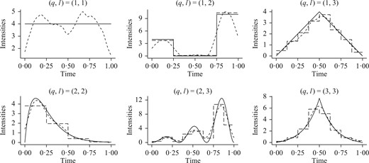
Intensities in synthetic experiments from Scenario 2 with |$n= 50$|⁠: each panel displays, for a pair of groups |$(q,l)$| with |$q,l=1,2, 3$| and |$q\le l$|⁠, the true intensity (solid) along with the kernel (dotted) and histogram (dashed) estimates for one simulated dataset selected at random.

For each parameter setting, our algorithm is applied to 1000 simulated datasets. The histogram estimator is used with regular dyadic partitions and |$d_{\max}=3$|⁠, while the kernel estimator uses the Epanechnikov kernel.

To assess the clustering performance, we use the adjusted Rand index (Hubert & Arabie, 1985), which measures the agreement between the estimated and true latent structures. For two classifications that are identical up to label switching, this index equals |$1$|⁠; otherwise the adjusted Rand index is smaller than |$1$|⁠, and negative values are possible. Figure 2 shows boxplots of the adjusted Rand index obtained with the histogram and kernel versions of our method in Scenario 1. For small values of the shift parameter, |$\varphi \in \{0{\cdot}01,0{\cdot}05\}$|⁠, the intensities are so close that classification is very difficult, especially when |$n$| is small, i.e., |$n=10$|⁠. The classification improves when the shift between the intensities and/or the number of observations increases, with almost perfect classification achieved for larger values of |$\varphi$| and/or |$n$|⁠.

Fig. 2.

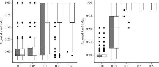
Boxplots of the adjusted Rand index in synthetic experiments from Scenario 1 for the histogram (grey) and kernel (white) estimators. The horizontal axis represents different values of the shift parameter |$\varphi$|⁠.

Concerning the recovery of the intensities in Scenario 2, we define the risk measuring the distance between the true intensity |$\alpha^{(q,l)}$| and its estimate |$\hat{\alpha}^{(q,l)}$| as

\begin{equation*} {\small{\text{RISK}}}(q,l)=\| \hat{\alpha}^{(q,l)} - \alpha^{(q,l)} \|_2= \left[\int_0^T \{ \hat{\alpha}^{(q,l)}(t) - \alpha^{(q,l)}(t) \}^2 \,{\mathrm{d}} t \right]^{1/2}\text{.} \end{equation*}

Table 1 reports mean values and standard deviations of the risk when |$n=50$|⁠. Our histogram and kernel estimators are compared with their oracle equivalents obtained using knowledge of the true groups. The table also reports the mean number of events with latent groups |$(q,l)$|⁠. As expected, when the true intensity is piecewise constant, the histogram version of our method outperforms the kernel estimator. Conversely, when the true intensity is smooth, the kernel estimator is better at recovering the shape of the intensity. Both estimators perform well compared with the oracle versions.

Table 1.

Mean numbers of events and risks (with standard deviations in parentheses) in Scenario|$\;2$| with |$n=50$|⁠; histogram and kernel estimators are compared with their oracle counterparts; all values associated with the risks are multiplied by |$100$|

Groups |$(q,l)$|	Nb.events	Hist (sd)	Or.Hist (sd)	Ker (sd)	Or.Ker (sd)
|$(1,1)$|	543	31 (32)	20 (18)	81 (51)	63 (12)
|$(1,2)$|	949	44 (17)	81 (4)	172 (57)	156 (7)
|$(1,3)$|	545	46 (16)	38 (6)	53 (88)	21 (6)
|$(2,2)$|	212	69 (10)	70 (9)	50 (56)	35 (11)
|$(2,3)$|	844	187 (6)	185 (2)	125 (56)	106 (11)
|$(3,3)$|	298	83 (13)	81 (13)	64 (53)	43 (12)

Nb.events, mean number of events; sd, standard deviation; Hist, histogram estimator; Ker, kernel estimator; Or.Hist, oracle counterpart of the histogram estimator; Or.Ker, oracle counterpart of the kernel estimator.

We use Scenario 2 to illustrate the performance of the integrated classification likelihood criterion in selecting the number |$Q$| of latent groups from the data. For each of the 1000 simulated datasets, the maximizer |$\hat Q$| of the integrated classification likelihood criterion defined in (10) with |$Q_{\max}=10$| is computed. For |$n=20$| the correct number of groups is recovered in 74% of the cases; the remaining cases select values in |$\{2,4\}$|⁠. Moreover, for datasets where the criterion does not select the correct number |$Q$|⁠, the adjusted Rand index of the classification obtained with three groups is rather low, indicating that the algorithm has failed in the classification task and that probably only a local maximum of |$J$| has been found.

For |$n=50$| our procedure selects the correct number of groups in 99|$\cdot$|9% of the cases.

5. Datasets

5.1. London bicycles dataset

We analyse cycle hire usage data from the bike-sharing system in the city of London from 2012 to 2015 (Transport for London, 2016). We focus on two randomly chosen weekdays, 1 and 2 February 2012, which we call day 1 and day 2, respectively. The data consist of pairs of stations associated with a single hiring/journey, identified by the starting station, ending station and corresponding time stamp, defined as the hire starting time expressed in seconds. The datasets were pre-processed to remove journeys that either correspond to loops, last less than 1 minute or more than 3 hours, or do not have an ending station. The datasets contain |$n_1=415$| and |$n_2=417$| stations on day 1 and day 2 with |$M_1=17\,631$| and |$M_2= 16\,333$| hire events, respectively. With more than |$17\times 10^4$| oriented pairs of stations, the number of processes |$N_{i,j}$| is huge, but only around 7% of these processes are nonnull, i.e., contain at least one hiring event between these stations. Indeed, bike-sharing systems are mostly used for short trips, and stations far from each other are unlikely to be connected. The data correspond to origin/destination flows and are analysed in a directed set-up using the histogram version of our algorithm on a regular dyadic partition with maximum size 32 corresponding to |$d_{\max} =5$|⁠.

The integrated classification likelihood criterion achieves its maximum with |$\hat Q=6$| latent groups for both datasets. Geographic locations of the bike stations and the clusters can be represented on a city map, thanks to the OpenStreetMap project; see Fig. 3 for day 1. Clusters for day 2 are similar, so we focus on day 1. Our procedure globally recovers geographic clusters, as interacting stations are expected to be near each other. While all clusters but one contain between 17 and 202 stations, cluster 4, shown with dark blue crosses in Fig. 3, consists of only two bike stations, at King’s Cross and Waterloo railway stations, which are among the stations showing the highest activity in terms of both departures and arrivals relative to all other stations. These stations appear to be outgoing stations in the morning, with many more departures than arrivals around 8 a.m., and to be incoming stations at the end of the working day, with more arrivals than departures between 5 p.m. and 7 p.m. The bike stations close to the other two main railway stations in London, Victoria and Liverpool Street stations, do not exhibit the same pattern and are clustered differently despite having a large number of hiring events. Cluster 4 is thus created from the similarity of the temporal profiles of these two stations rather than their total quantity of interactions. Moreover, it mostly interacts with cluster 5, which roughly corresponds to the City of London neighbourhood. It is therefore characterized by stations used by people living in the suburbs and working in the city.

Fig. 3.

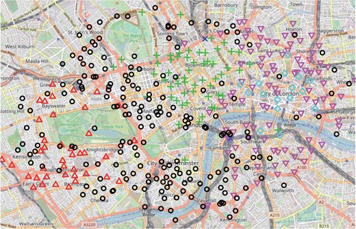
Map of London bike-sharing system, showing the geographic locations of the stations and clustering for day 1: cluster 1 (red triangles), cluster 2 (black circles), cluster 3 (green crosses), cluster 4 (dark blue crosses), cluster 5 (light blue diamonds), and cluster 6 (pink triangles).

We compare our method with the discrete-time approach of Matias & Miele (2017), where individuals are allowed to change groups over time. We applied the R package dynsbm to the London bikes dataset, aggregated into |$T=24$| snapshots of length one hour, but no similar results emerged. The model selection criterion of Matias & Miele (2017) chooses four groups; the clusters with |$Q=4$| groups drop to only one nonempty group between midnight and 3 a.m., two groups between 3 a.m. and 7 a.m., and three groups between 10 p.m. and midnight. Globally there is one very large group, containing from 168 to all stations, one medium-size group with 0 to 148 stations, and two small groups with 0 to 62 and 64 stations. Our small cluster is not detected by the dynsbm method.

The same dataset was analysed in Guigourès et al. (2015) from a different perspective. Randriamanamihaga et al. (2014) rely on Poisson mixture models to analyse the bike-sharing system in Paris. Their approach does not take into account the network structure of the data, where, for instance, two flows from the same station are related. As a consequence, clusters are obtained on pairs of stations, so their interpretation is completely different from ours and in a way less natural.

5.2. Enron dataset

The Enron corpus contains email exchanges between people working at Enron, mostly in senior management, covering the period of the affair that led to the bankruptcy of the company (Klimt & Yang, 2004). From the data provided by the CALO Project (2015) we extracted 21 267 emails exchanged among 147 persons between 27 April 2000 and 14 June 2002, for which the sender, the recipient and the time when each email was sent are known. For most people, their position in the company is known: one out of four are employees, while all other positions involve responsibility and we summarize them as managers.

We applied our algorithm using the directed model and the histogram approach with regular dyadic partitions of maximal size 256, corresponding to |$d_{\max}=8$|⁠. For each fixed number of groups |$Q\in\{2,\ldots,20\}$|⁠, the algorithm identifies one large group, which always contains the same individuals. One could consider this group as having the standard behaviour at the company. For varying values of |$Q$| the differences in the clustering only concern the remaining individuals with nonstandard behaviour. The integrated classification likelihood criterion does not provide a reasonably small enough number of groups that could be used for interpretation. We therefore choose to analyse the data with |$Q=4$| clusters. The group with the standard behaviour, group 1, contains 127 people, both employees and managers. The second largest group, group 4, contains managers almost exclusively, and group 2 is composed of employees. The standard behaviour of group 1 consists in receiving mails from all other groups but with little sending activity. The members of group 3 have the greatest intensity of email exchanges. The specific manager and employee groups, i.e., groups 2 and 4, are quite similar, and indeed at |$Q=3$| they merge. For a number of pairs of groups communication is relatively constant over time, but for others the activity evolves a lot, e.g., emails sent to members of group 1; see Fig. 4. The intragroup intensity of group 1 increased over time, with a peak in October 2001, which coincides with the beginning of the investigations relating to the scandal. In contrast, the managers of group 4 communicated more intensely with group 1 during the first half of the observation time than during the later half. More details are provided in the Supplementary Material.

Fig. 4.

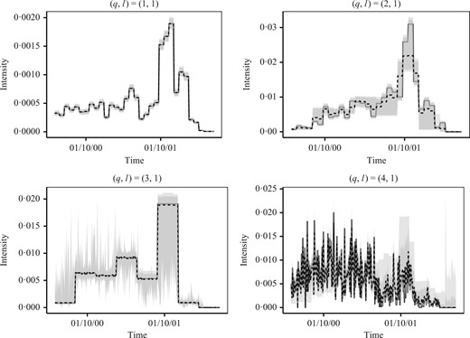
The Enron dataset: intensity estimates for pairs of groups |$(q,1)$| for |$q\in\{1,\ldots,4\}$| and bootstrap confidence intervals with confidence level 90% (light grey) or 80% (dark grey); in each panel the dashed line represents the median value of the 80% confidence interval.

The confidence intervals in Fig. 4 were obtained via a parametric bootstrap. In general, the confidence intervals are satisfactory for large groups but not for small groups. Indeed, some of the estimated probabilities |$\hat \pi_k$| of group membership are very small, with two being lower than 3%, so bootstrap samples tend to have empty groups, which ruins the associated bootstrap intervals.

Rastelli et al. (2017) analysed the same dataset with a discrete-time model where individuals may change groups over time. They also found that most individuals assemble in one group, corresponding to people who were rather inactive but were receiving emails. They also observed a specific behaviour of some groups of employees and managers. However, there is a difference in the interpretation of results from the two models. In Rastelli’s model, groups may be identified with specific tasks, such as sending newsletters, and individuals may execute this task for a while and then change activity. In contrast, our model identifies groups of individuals with similar behaviour over the entire observation period. Thus our approach is more natural for analysing the temporal evolution of the activity of a fixed group of persons.

Finally, we carried out a comparison with a classical stochastic block model. Taking |$d_{\max}=0$| in our approach amounts to forgetting the time stamps of the emails, as the algorithm then only considers email counts over the whole observation period, and our method boils down to a classical stochastic block model with Poisson emission distribution and mean parameter |$A^{(q,l)} (T)$| (Mariadassou et al., 2010). Comparing the classification at |$Q=4$| with that obtained using our continuous-time approach, the adjusted Rand index equals 0|$\cdot$|798, indicating that the clusterings are different. Both models roughly identify the same large group with standard behaviour, but huge differences appear in the classification of the nonstandard individuals. Thus our approach does use the temporal distribution of events to cluster the individuals. The higher value of the complete loglikelihood in the Poisson process stochastic block model indicates that the solution is indeed an improvement over the classical model.

Acknowledgement

We thank Agathe Guilloux for pointing out valuable references, Nathalie Eisenbaum for her help on doubly stochastic counting processes and Pierre Latouche for sharing information on datasets. The computations were partly performed at the Institute for Computing and Data Sciences at Sorbonne University.

Supplementary material

Supplementary material available at Biometrika online includes a model that accounts for sparse datasets, proofs of the theoretical results, technical details of the methods and algorithm, the study of a third dataset, code in R the corresponding R package, named ppsbm, has been released on CRAN.

Author notes

C. Matias,

F. Villers,