In search of lost mixing time: adaptive Markov chain Monte Carlo schemes for Bayesian variable selection with very large p

Summary

The availability of datasets with large numbers of variables is rapidly increasing. The effective application of Bayesian variable selection methods for regression with these datasets has proved difficult since available Markov chain Monte Carlo methods do not perform well in typical problem sizes of interest. We propose new adaptive Markov chain Monte Carlo algorithms to address this shortcoming. The adaptive design of these algorithms exploits the observation that in large-|$p$|⁠, small-|$n$| settings, the majority of the |$p$| variables will be approximately uncorrelated a posteriori. The algorithms adaptively build suitable nonlocal proposals that result in moves with squared jumping distance significantly larger than standard methods. Their performance is studied empirically in high-dimensional problems and speed-ups of up to four orders of magnitude are observed.

1. Introduction

The availability of large datasets has led to an increasing interest in variable selection methods applied to regression models with many potential variables, but few observations, so-called large-|$p$|⁠, small-|$n$| problems. Frequentist approaches have mainly concentrated on point estimates under assumptions of sparsity using penalized maximum likelihood procedures (Hastie et al., 2015). Bayesian approaches to variable selection are an attractive and natural alternative, and lead to a posterior distribution on all possible models which can address model uncertainty for variable selection and prediction. A growing literature provides a theoretical basis for good posterior properties in large-|$p$| problems (see, e.g., Johnson & Rossell, 2012; Castillo et al., 2015).

The posterior probabilities of all possible models can usually only be calculated or approximated if |$p$| is smaller than 30. If |$p$| is larger, Markov chain Monte Carlo methods are typically used to sample from the posterior distribution (George & McCulloch, 1997; O’Hara & Sillanpää, 2009; Clyde et al., 2011). García-Donato & Martínez-Beneito (2013) discuss the benefits of such methods. The most widely used Markov chain Monte Carlo algorithm in this context is the Metropolis–Hastings sampler, where new models are proposed using add-delete-swap samplers (Brown et al., 1998; Chipman et al., 2001). For example, this approach is used by Nikooienejad et al. (2016) in a binary regression model with a nonlocal prior for the regression coefficients on a dataset with 7129 genes. Some supporting theoretical understanding of convergence is available for the add-delete-swap samplers, e.g., conditions for rapid mixing in linear regression models have been derived by Yang et al. (2016). Others have considered more targeted moves in model space. For example, Titsias & Yau (2017) introduce the Hamming ball sampler which more carefully selects the proposed model in a Metropolis–Hastings sampler, in a similar way to shotgun variable selection (Hans et al., 2007), and Schäfer & Chopin (2013) develop a sequential Monte Carlo method that uses a sequence of annealed posteriors. Several authors use more general shrinkage priors and develop suitable Markov chain Monte Carlo algorithms for high-dimensional problems (see, e.g., Bhattacharya et al., 2016). Nonlocal priors (Johnson & Rossell, 2012) are adopted in Shin et al. (2018), who use screening for high dimensions. Zanella & Roberts (2019) combine Markov chain Monte Carlo and importance sampling ideas in their tempered Gibbs sampler.

The challenge of performing Markov chain Monte Carlo for Bayesian variable selection in high dimensions has led to several developments sacrificing exact posterior exploration. For example, Liang et al. (2013) use the stochastic approximation Monte Carlo algorithm (Liang et al., 2007) to efficiently explore model space. In another direction, variable selection can be performed as a post-processing step after fitting a model including all variables (see, e.g., Bondell & Reich, 2012; Hahn & Carvalho, 2015). Several authors develop algorithms that focus on high posterior probability models. In particular, Rockova & George (2014) propose a deterministic expectation-maximization-based algorithm for identifying posterior modes, while Papaspiliopoulos & Rossell (2017) develop an exact deterministic algorithm to find the most probable model of any given size in block-diagonal design models.

Alternatively, Markov chain Monte Carlo methods for variable selection can be tailored to the data to allow faster convergence and mixing using adaptive ideas (see, e.g., Green et al., 2015, § 2.4, and references therein). Several strategies have been developed in the literature for both the Metropolis-type algorithms (Ji & Schmidler, 2013; Lamnisos et al., 2013) and Gibbs samplers (Nott & Kohn, 2005; Richardson et al., 2010). Our proposal is a Metropolis–Hastings kernel that learns the relative importance of the variables, unlike previous work (see, e.g., Ji & Schmidler, 2013; Lamnisos et al., 2013). A similar strategy is used by Zanella & Roberts (2019) in a Gibbs sampling framework. This leads to substantially more efficient algorithms than commonly used methods in high-dimensional settings, and for which the computational cost of one step scales linearly with |$p$|⁠. The algorithms adaptively build suitable nonlocal Metropolis–Hastings-type proposals that result in moves with expected squared jumping distance (Gelman et al., 1996) significantly larger than standard methods. In idealized examples the limiting versions of our adaptive algorithms converge in |$\mathcal{O}(1)$| and result in super-efficient sampling. They outperform independent sampling in terms of the expected squared jump distance and also in the sense of the central limit theorem asymptotic variance. This is in contrast to the behaviour of optimal local random walk Metropolis algorithms that on analogous idealized targets need at least |$\mathcal{O}(p)$| samples to converge (Roberts et al., 1997). The performance of our algorithms is studied empirically in realistic high-dimensional problems for both synthetic and real data. In particular, in § 4.1, for a well-studied synthetic data example, speed-ups of up to four orders of magnitude are observed compared to standard algorithms. Moreover, in § 4.2, we show the efficiency of the method in the presence of multicollinearity on a real-data example with |$p=100$| variables, and in § 4.3, we present real-data gene expression examples with |$p=22\, 576$| and with |$p=79\, 748$|⁠, and reliably estimate the posterior inclusion probabilities for all variables. The Supplementary Material has results from three datasets with moderate |$p$| and high correlations used in Schäfer & Chopin (2013), indicating that our algorithms outperform most other methods in the literature. The algorithms have the potential to be parallelized across the multiple chains and to be applied to non-Gaussian models or more general prior structures.

2. Design of the adaptive samplers

2.1. The setting

Our approach is applicable to general regression settings, but we will focus on normal linear regression models. This will allow for clean efficiency comparisons independent of model-specific sampling details, e.g., of a reversible jump implementation. We define |$\gamma=(\gamma_1,\dots,\gamma_p) \in \Gamma = \{0,1\}^p$| to be a vector of indicator variables with |$\gamma_i=1$| if the |$i$|th variable is included in the model and |$p_{\gamma}=\sum_{j=1}^p \gamma_j$|⁠. We consider the model specification

$$\begin{equation*} y=\alpha 1_n + X_{\gamma}\beta_{\gamma} + e,\qquad e\sim{{N}}(0,\sigma^2 I_n) , \end{equation*}$$

where |$y$| is an |$(n\times 1)$|-dimensional vector of responses, |$a_q$| represents a |$q$|-dimensional column vector with entries |$a$|⁠, and |$X_\gamma$| is an |$(n\times p_\gamma)$|-dimensional data matrix formed using the included variables. We consider Bayesian variable selection and, for clarity of exposition and validity of comparisons, we will assume the commonly used prior structure

$$\begin{equation}p(\alpha,\sigma^2,\beta_{\gamma},\gamma)\propto \sigma^{-2}\,p(\beta_{\gamma}\mid\sigma^2, \gamma)\,p(\gamma) , \label{prior} \end{equation}$$

(1)

with |$\beta_{\gamma} \mid \sigma^2,\gamma \sim {{N}}(0,\sigma^2 V_{\gamma})$|⁠, and |$p(\gamma) = h^{p_{\gamma}}(1-h)^{p-p_{\gamma}}$|⁠. The hyperparameter |$0<h<1$| is the prior probability that a particular variable is included in the model, and |$V_{\gamma}$| is often chosen as proportional to |$(X_\gamma^{ \mathrm{\scriptscriptstyle T} } X_\gamma)^{-1}$|⁠, a |$g$|-prior, or to the identity matrix. In both cases, the marginal likelihood |$p(y\mid \gamma)$| can be calculated analytically. The prior can be further extended with hyperpriors, for example adopting |$h\sim{\mbox{Be}}(a,b)$|⁠.

We will consider sampling from the target distribution |$\pi_p(\gamma)=p(\gamma\mid y)$| using a nonsymmetric Metropolis–Hastings kernel. Let the probability of proposing to move from model |$\gamma$| to |$\gamma'$| be

$$\begin{equation} q_{\eta}(\gamma,\gamma')=\prod_{j=1}^p q_{\eta,\ j}(\gamma_j,\gamma'_j) , \label{gen_prop} \end{equation}$$

(2)

where |$\eta = (A,D) = (A_1,\dots, A_p, D_1, \dots, D_p)$|⁠, |$q_{\eta,\ j}(\gamma_j=0, \gamma_j'=1)=A_j$| and |$q_{\eta,\ j} (\gamma_j=1,\gamma_j'=0)=D_j$|⁠. The proposal can be quickly sampled, the parameterization allows optimization of the expected squared jumping distance, and multiple variables can be added to or deleted from the model in one iteration. The proposed model is accepted using the standard Metropolis–Hastings acceptance probability

$$\begin{equation*} a_{\eta}(\gamma,\gamma') = \min\left\{1,\frac{\pi_p(\gamma') q_{\eta}(\gamma',\gamma)}{\pi_p(\gamma) q_{\eta}(\gamma,\gamma')}\right\}\!. \end{equation*}$$

2.2. In search of lost mixing time: optimizing the sampler

The transition kernel in (2) is highly parameterized, with |$2p$| parameters, and these will be tuned using adaptive Markov chain Monte Carlo methods (see, e.g., Andrieu & Thoms, 2008; Roberts & Rosenthal, 2009; Green et al., 2015). These methods allow the tuning of parameters on the fly to improve mixing using some computationally accessible performance criterion whilst maintaining the ergodicity of the chain. Suppose that |$\mu_p$| is a |$p$|-dimensional probability density function which has the form |$\mu_p = \prod_{j=1}^p f$|⁠. A commonly used result is that the optimal scale of a random walk proposal for |$\mu_p$| leads to a mean acceptance rate of |$0.234$| as |$p\rightarrow\infty$| for some smooth enough |$f$|⁠. The underlying analysis also implies that the optimized random walk Metropolis will converge to stationarity in |$\mathcal{O}(p)$| steps. This is a useful guide even in moderate dimensions, and well beyond the restrictive independent, identically distributed product form assumption of Roberts et al. (1997). Lamnisos et al. (2013) show that this rule can be effectively used to tune a Metropolis–Hastings sampler for Bayesian variable selection. However, other results suggest that other optimal scaling rules could work well in Bayesian variable selection problems. Firstly, Neal et al. (2012) establish, under additional regularity conditions, that if |$f$| is discontinuous, the optimal mean acceptance rate for a Metropolis–Hastings random walk is |${\rm e}^{-2}\approx 0.1353$| and the chain mixes in |$\mathcal{O}(p^2)$| steps, an order of magnitude slower than with smooth target densities |$f$|⁠. Rather surprisingly, Lee & Neal (2018) show that the optimally tuned independence sampler in this setting recovers the |$O(p)$| mixing and acceptance rate of |$0.234$| without any additional smoothness conditions. Secondly, Roberts (1998) considers optimal scaling of the random walk Metropolis–Hastings algorithm on |$\Gamma=\{0,1\}^p$| for the product measures

$$\begin{equation*} \mu_p(\gamma_1, \dots, \gamma_p) = s^{p_\gamma}(1-s)^{p- p_\gamma},\qquad \gamma=(\gamma_1,\dots,\gamma_p)\in\Gamma, \quad 0<s<1. \end{equation*}$$

If |$s$| is close to |$1/2$|⁠, the optimal |$\mathcal{O}(p)$| mixing rate occurs as |$p$| tends to infinity if the mean acceptance rate is |$0.234$|⁠. If |$s\rightarrow 0$| as |$p\rightarrow \infty$|⁠, the numerical results of Roberts (1998, § 3) indicate that the optimally tuned random walk Metropolis proposes to change two |$\gamma_j$|s at a time, but that the acceptance rate deteriorates to zero resulting in the chain not moving. This suggests that the actual mixing in this regime is slower than the |$\mathcal{O}(p)$| observed for smooth continuous densities.

In Bayesian variable selection, it is natural to assume that the variables differ in posterior inclusion probabilities and so we consider target densities that have the form

$$\begin{equation}\label{our-target} \pi_p(\gamma) = \prod_{j=1}^{p}\pi_j^{\gamma_j}(1-\pi_j)^{1-\gamma_j},\qquad \gamma\in\Gamma , \end{equation}$$

(3)

where |$0<\pi_j<1$| for |$j=1,\dots,p$|⁠. Consider the nonsymmetric Metropolis–Hastings algorithm with the product form proposal |$q_{\eta}(\gamma, \gamma')$| given by (2) targeting the posterior distribution given by (3). Note that |$\alpha_{\eta}(\cdot \, , \cdot) \equiv 1$| for any choice of |$\eta = (A,D)$|⁠, satisfying

$$\begin{equation}\label{accept1} \frac{A_j}{D_j} = \frac{\pi_j}{1-\pi_j} \qquad \textrm{for every } j. \end{equation}$$

(4)

To discuss optimal choices of |$\eta$|⁠, we consider several commonly used criteria for Markov chains with stationary distribution |$\pi$| and transition kernel |$P$| on a finite discrete state space |$\Gamma$|⁠. The mixing time of a Markov chain (Roberts & Rosenthal, 2004) is |$ \rho := \min\{t: \max_{\gamma \in \Gamma} \|P^t(\gamma, \cdot) - \pi(\cdot)\|_{\rm TV} < 1/2\} , $| where |$\|\cdot\|_{\rm TV}$| is the total variational norm. If |$\Gamma = \{0,1\}^p$|⁠, it is natural to define the expected squared jumping distance (Gelman et al., 1996) as |${E}_{\pi}\big(\sum_{j=1}^p \big\vert\gamma^{(0)}_j - \gamma^{(1)}_j\big\vert^2\big)$|⁠, where |$\gamma^{(0)}$| and |$\gamma^{(1)}$| are two consecutive values in a Markov chain trajectory, which is the average number of variables changed in one iteration. Suppose that the Markov chain is ergodic; then, for any function |$f: \Gamma \to \mathbb{R}$|⁠, |$ \frac{1}{\surd{n}}\sum_{k=0}^{n-1} f(\gamma^{(k)}) \stackrel {D}{\rightarrow} N(E_{\pi}f, \sigma^2_{P,\ f}), $| where the constant |$\sigma^2_{P,\ f}$| depends on the transition kernel |$P$| and function |$f$|⁠. Consider transition kernels |$P_1$| and |$P_2$|⁠. If |$\sigma^2_{P_1,f} \leqslant \sigma^2_{P_2,f} $| for every |$f,$| then |$P_1$| dominates |$P_2$| in Peskun ordering (Peskun, 1973). If |$P_1$| dominates all other kernels from a given class, then |$P_1$| is optimal in this class with respect to Peskun ordering. Apart from toy examples, Peskun ordering can rarely be established without further restrictions. Hence, for the variable selection problem, where posterior inclusion probabilities are often of interest, we consider Peskun ordering for the class |$\mathbb{L}(\Gamma)$| of linear combinations of univariate functions,

$$\begin{equation} \label{lin_fun}\mathbb{L}(\Gamma) := \bigg\{f:\Gamma \to \mathbb{R}: f(\gamma) = a_0 + \sum_{j=1}^p a_j f_j(\gamma_j) \bigg\}. \end{equation}$$

(5)

We consider two proposals which satisfy (4): the independent proposal for which |$A_j=1-D_j=\pi_j $|⁠, and the informed proposal for which |$A_j = \min\big(1, \frac{\pi_j}{1-\pi_j}\big)$| and |$D_j = \min\big(1, \frac{1- \pi_j}{\pi_j}\big)$|⁠. The following proposition shows that the informed proposal has more desirable properties.

 

Proposition 1.

Consider the class of Metropolis–Hastings algorithms with target distribution given by (3), and proposal |$q_{\eta}(\gamma, \gamma')$| given by (2) with the independent or informed proposal. Let |${\rm var}_{\pi}f $| be the stationary variance of |$f$| under |$\pi_p(\gamma)$| and |$\pi^{(j)} := \{1-\pi_j, \pi_j\}$|⁠. Then:  

• (i) The independent proposal leads to

  • (a) independent sampling and optimal mixing time |$\rho = 1$|⁠;

  • (b) the expected squared jumping distance |$E_{\pi}(\Delta^2) = 2\sum_{j=1}^p \pi_j(1-\pi_j)$|⁠;

  • (c) the asymptotic variances |$\sigma_{P,\ f}^2 = {\rm var}_{\pi}f$| for arbitrary |$f$| and |$\sigma_{P,\ f}^2 = {\rm var}_{\pi}f = \sum_{j=1}^p a_j^2 {\rm var}_{\pi^{(j)}}f_j$| for |$f \in \mathbb{L}(\Gamma)$|⁠.

• (ii) The informed proposal leads to

  • (a) the expected squared jumping distance |$E_{\pi}(\Delta^2) = 2\sum_{j=1}^p\min(1-\pi_j, \pi_j)$|⁠, which is maximal;

  • (b) the asymptotic variance |$\sigma_{P,\ f}^2 = \sum_{j=1}^p \left\{2 \max (1-\pi_j, \pi_j) -1 \right\}a_j^2 {\rm Var}_{\pi^{(j)}}f_j$| for |$f \in \mathbb{L}(\Gamma)$|⁠, which is optimal with respect to the Peskun ordering for the class of linear functions |$\mathbb{L}(\Gamma)$| defined in (5).

 

Remark 1.

The differences of the expected squared jumping distance and asymptotic variance for the two proposals is largest when |$\pi_j$| is close to |$1/2$|⁠.

 

Remark 2.

In discrete spaces, Schäfer & Chopin (2013) argue that the mutation rate

$$\begin{equation*} \bar{a}_{\rm M}=\int \mathbb{I}(\gamma~{\rm =}\kern-0.5em{\rm |}~ \gamma')\,a_\eta(\gamma,\gamma')\,q_{\eta}(\gamma,\gamma')\,\pi(\gamma) \,{\rm d}\gamma'\,{\rm d}\gamma, \end{equation*}$$

which excludes moves which do not change the model, is more appropriate than the average acceptance rate. The mutation rate is |$ \bar{a}_{\rm M} =1 - \prod_{j=1}^p\big \{ (1 - \pi_j)^2 + \pi_j^2 \big\}$| with independent sampling and |$ \bar{a}_{\rm M} =1 - \prod_{j=1}^p \vert 2\pi_j-1\vert$| with the informed proposal. Therefore, the informed proposal always leads to a higher mutation rate.

 

Remark 3.

Zanella (2020) discusses a framework for designing informed proposals in discrete spaces, and discusses optimal choices under Peskun ordering.

These results suggest that the informed proposal should be preferred to the independent proposal when designing a Metropolis–Hastings sampler for idealized posteriors of the form in (3). In practice, the posterior distribution will not have a product form, but can anything be said about its form when |$p$| is large? The following result sheds some light on this issue. We define |${\rm BF}_j(\gamma_{-j})$| to be the Bayes factor of including the |$j$|th variable given the values of |$\gamma_{-j}=(\gamma_1,\dots,\gamma_{j-1},\gamma_{j+1},\dots,\gamma_p)$| and denote by |$\gamma_0$| the vector |$\gamma$| without |$\gamma_j$| and |$\gamma_k$|⁠.

 

Proposition 2.

Let |$a=\frac{{\rm BF}_j(\gamma_k=1,\gamma_0)} {{\rm BF}_j(\gamma_k=0,\gamma_0)}$|⁠. If (i) |$a \rightarrow 1$| or (ii) |$a\rightarrow A<\infty$| and |${\rm BF}_j(\gamma_k=0,\gamma_{0}) h\rightarrow 0$| then |$ p(\gamma_j=1\mid \gamma_k=1,\gamma_0) \rightarrow p(\gamma_j=1\mid \gamma_k=0,\gamma_0)$|⁠.

This result gives conditions under which |$\gamma_j$| and |$\gamma_k$| are approximately independent. Condition (ii) is interesting in large |$p$| settings: |$\gamma_j$| and |$\gamma_k$| are approximately independent if |$p$| is large, and so |$h$| is small, and |${\rm BF}_j(\gamma_k=0,\gamma_{0})$| is not large, i.e., the evidence in favour of including |$\gamma_j$| is not large. This will be the case for all variables apart from the most important. Although this result provides some reassurance, there will be some posterior correlation in many problems, and the informed proposal may propose changing too many variables, leading to low acceptance rates. This can be addressed by using a scaled proposal of the form

$$\begin{equation}\label{individually_scaled} A_j = \zeta_j \min\left(1, \frac{\pi_j}{1-\pi_j}\right), \qquad D_j = \zeta_j \min\left(1, \frac{1- \pi_j}{\pi_j}\right). \end{equation}$$

(6)

The family of these proposals for |$\zeta_j \in [0,1]$| form a line segment for |$(A_j, D_j)$| between |$(0, 0)$| and |$\big\{\min\big(1, \frac{\pi_j}{1-\pi_j}\big), \min\big(1, \frac{1- \pi_j}{\pi_j}\big)\big\}$|⁠, which is illustrated in Fig. 1. The independent proposal corresponds to the point on this line where |$\zeta_j=\max(\pi_j, 1-\pi_j)$|⁠.

Fig. 1.

The solid black line shows pairs |$(A_j, D_j)$| corresponding to |$\pi=1/3$| and |$\zeta_j \in [0,1]$| in (6). The independent proposal (i), marked with a triangle, is a shrunk version of the informed proposal (ii), marked with a bullet.

In the next section we devise adaptive Markov chain Monte Carlo algorithms to tune proposals of the form (2) so that the |$A_j$| and |$D_j$| lie approximately on this line. Larger values of |$\zeta_j$| tend to lead to larger jumps, whereas smaller values of |$\zeta_j$| tend to increase acceptance. These algorithms aim to find a point which balances this trade-off. We define two strategies for adapting |$\eta$|⁠: exploratory individual adaptation and adaptively scaled individual adaptation.

With both forms of adaptation, we run independent parallel chains which share the same proposal parameters and refer to this as multiple-chain acceleration. Craiu et al. (2009) show empirically that running multiple independent Markov chains with the same adaptive parameters improves the rate of convergence of adaptive algorithms towards their target acceptance rate in the context of the classical adaptive Metropolis algorithm of Haario et al. (2001); see also Bornn et al. (2013).

At this point, it is helpful to define some notation. Let |$\eta^{(i)}=(A^{(i)},D^{(i)})$| and |$\gamma^{(i)}$| be the values of |$\eta$| and |$\gamma$| at the start of the |$i$|th iteration, and |$\gamma'$| be the subsequently proposed value. Let |$ a_i = a_{\eta^{(i)}}(\gamma^{(i)}, \gamma')$| be the acceptance probability at the |$i$|th iteration. We define, for |$j=1,\dots,p$|⁠,

$$\begin{align*} \gamma^{A\,(i)}_j= \left\{\begin{array}{ll} 1\mbox{ if }\gamma'_j~{\rm =}\kern-0.5em{\rm |}~ \gamma_j^{(i)}\mbox{ and }\gamma_j^{(i)}=0 , \\ 0\mbox{ otherwise} ; \end{array}\right. \qquad \gamma^{D\,(i)}_j= \left\{\begin{array}{ll} 1\mbox{ if }\gamma'_j~{\rm =}\kern-0.5em{\rm |}~ \gamma_j^{(i)}\mbox{ and }\gamma_j^{(i)}=1 , \\ 0\mbox{ otherwise} , \end{array}\right. \end{align*}$$

and the map |${\mbox{logit}}_{\epsilon}: (\epsilon,1-\epsilon)\rightarrow \mathbb{R}$| by |$ {\mbox{logit}}_{\epsilon}(x) = \log(x-\epsilon) - \log(1 - x - \epsilon), $| where |$0\leqslant\epsilon\leqslant1/2$|⁠. This reduces to the usual logit transform if |$\epsilon=0$|⁠.

2.3. Remembrance of things past: exploratory individual adaptation

The first adaptive strategy is a general purpose method that we term exploratory individual adaptation. It aims to find pairs |$(A_j, D_j)$| on the line segment defined by (4) which lead to good mixing. Proposals with larger values of |$A_j$| and |$D_j$| will tend to propose more changes to the included variables, but will also tend to reduce the average acceptance probability or mutation rate. The method introduces two tuning parameters, |$\tau_{\rm L}$| and |$\tau_{\rm U}$|⁠. There are three types of updates for |$A^{(i)}$| and |$D^{(i)}$| which move towards the correct ratio |$A_j/D_j$| and then along the segment, where the slope of the segment depends on |$\pi_j$|⁠. Unless otherwise stated, |$A^{(i+1)}_j=A^{(i)}_j$| and |$D^{(i+1)}_j=D^{(i)}_j$|⁠.

Both the expansion step and the shrinkage step change |$A^{(i+1)}_j$|⁠, and |$D^{(i+1)}_j$| for |$j$| in |$\gamma^{A(i)}$| and |$\gamma^{D(i)}$| to adjust the average squared jumping distance whilst maintaining that |$A^{(i+1)}_j / D^{(i+1)}_j \approx A^{(i)}_j / D^{(i)}_j$|⁠. The expansion step is used if a promising move is proposed, when |$a_i>\tau_{\rm U}$|⁠, and sets |$A^{(i+1)}_j$| and |$D^{(i+1)}_j$| larger than |$A^{(i)}_j$| and |$D^{(i)}_j$|⁠, respectively. Similarly, the shrinkage step is used if an unpromising move has been proposed, when |$a_i<\tau_{\rm L}$|⁠, and |$A^{(i+1)}_j$| and |$D^{(i+1)}_j$| are set smaller than |$A^{(i)}_j$| and |$D^{(i)}_j$|⁠.

The correction step aims to increase the average acceptance rate by correcting the ratio between |$A$| and |$D$|⁠. If |$\tau_{\rm L}<a_i<\tau_{\rm U}$|⁠, we set |$A^{(i+1)}_j>A^{(i)}_j$| and |$D^{(i+1)}_j<D^{(i}_j$| if |$\gamma^{D(i)}_j=1$|⁠, and |$A^{(i+1)}_j<A^{(i)}_j$| and |$D^{(i+1)}_j>D^{(i)}_j$| if |$\gamma^{A(i)}_j=1$|⁠.

The following updates achieve these properties:

$$\begin{eqnarray} {\mbox{logit}}_{\epsilon}A^{(i+1)}_j& = &{\mbox{logit}}_{\epsilon}A^{(i)}_j + \phi_i \times\left[ \gamma^{A(i)}_j d_i(\tau_{\rm U}) + \gamma^{D(i)}_j d_i(\tau_{\rm L}) - \gamma^{A(i)}_j \{1-d_i(\tau_{\rm U})\}\right]\!, \label{eqn:adap_A} \\ \end{eqnarray}$$

(7)

 

$$\begin{eqnarray} {\mbox{logit}}_{\epsilon}D^{(i+1)}_j & = &{\mbox{logit}}_{\epsilon}D^{(i)}_j + \phi_i\times \left[ \gamma^{D(i)}_j d_i(\tau_{\rm U}) + \gamma^{A(i)}_j d_i(\tau_{\rm L}) - \gamma^{D(i)}_j \{1 - d_i(\tau_{\rm U})\}\right]\!, \label{eqn:adap_B} \end{eqnarray}$$

(8)

for |$j=1\dots,p$| where |$d_i(\tau) = \mathbb{I}\left(a_i\geqslant \tau\right)$| and |$\phi_i=O(i^{-\lambda})$| for some constant |$1/2<\lambda\leqslant 1$|⁠. The gradient fields of these updates are shown in the Supplementary Material. The transformation implies that |$\epsilon<A_j^{(i)}<1-\epsilon$| and |$\epsilon<D_j^{(i)}<1-\epsilon$|⁠, and we assume that |$0<\epsilon<1/2$|⁠. It also implies diminishing adaptation, since the derivative of the inverse logit is bounded; see Lemma 2. Based on several simulation studies, we suggest taking |$\tau_{\rm L} = 0.01$| and |$\tau_{\rm U} = 0.1$|⁠. As discussed in § 2.2, targeting a low acceptance rate is often beneficial in irregular cases, so we expect this choice to be robust in real data applications. In all our simulations with this parameter setting, the resulting mean acceptance rate was between |$0.15$| and |$0.35$|⁠, i.e., in the high efficiency region identified in Roberts et al. (1997). We also suggest an initial choice of parameters such that |$A_j^{(1)}/D_j^{(1)} \approx h/(1-h)$| as this summarizes the prior information on |$\pi_j / (1-\pi_j)$|⁠; in particular, |$D_j^{(1)}\equiv 1$| and |$A_j^{(1)}\equiv h$| often works well. The parameter |$\epsilon$| controls the minimum and maximum values of |$A_i$| and |$D_i$|⁠. In the large-|$p$| setting, |$A_i\approx\epsilon$| for unimportant variables and the expected number of those unimportant variables proposed to be included at each iteration will be approximately |$p\epsilon$|⁠, since the number of excluded, unimportant variables will be close to |$p$|⁠. This expected value can be controlled by choosing |$\epsilon=0.1/p$|⁠. The exploratory individual adaptation algorithm is described in Algorithm 1, and we indicate its transition kernel at time |$i$| as |$P_{\eta^{(i)}}^{\textrm{EIA}}$|⁠.

 

Algorithm 1.

Exploratory individual adaptation.

$$\begin{array} \qquad \textrm{for } i=\textrm{ 1 to }i=M\\ \qquad \qquad \textrm{sample } \gamma' \sim q_{\eta^{(i)}}(\gamma^{(i)}, \cdot) \textrm{ and } U \sim U(0,1);\\ \qquad \qquad \textrm{if } {U < a_{\eta^{(i)}}(\gamma^{(i)}, \gamma')} \textrm{ then } \gamma^{(i+1)}:=\gamma', \textrm{ else } \gamma^{(i+1)}:=\gamma^{(i)}; \\ \qquad \qquad \textrm{update } A^{(i+1)} \textrm{ using (7) and } D^{(i+1)} \textrm{ using (8) };\\ \textrm{endfor} \qquad \end{array}$$

2.4. Remembrance of things past: adaptively scaled individual adaptation

Algorithm 1 learns two parameters |$A_j^{(i)}$| and |$D_j^{(i)}$| for each variable and, we shall see, can slowly converge to optimal values if |$p$| is large. Alternatively, we could learn |$\pi_1,\dots,\pi_p$| from the chain to approximate the slope of the line defined by (4) and use the proposal (6) with the same scale parameter for all variables. We term this approach the adaptively scaled individual adaptation proposal. In particular, we use

$$\begin{equation} A_j^{(i)}=\zeta^{(i)}\min\big\{1,\hat\pi^{(i)}_j/\big(1-\hat\pi^{(i)}_j\big)\big\} \quad \mbox{and} \quad D_j^{(i)}=\zeta^{(i)}\min\big\{1,\big(1-\hat\pi^{(i)}_j\big)/\hat\pi^{(i)}_j\big\}, \label{ASI_update} \end{equation}$$

(9)

for |$j=1,\dots,p$|⁠, where |$0<\zeta^{(i)}<1$| is a tuning parameter and |$\hat\pi^{(i)}_j$| is a Rao–Blackwellized estimate of the posterior inclusion probability of variable |$j$| at the |$i$|th iteration. Like Ghosh & Clyde (2011), we work with the Rao–Blackwellized estimate conditional on the model, marginalizing over |$\alpha$|⁠, |$\beta_{\gamma}$| and |$\sigma^2$|⁠, in contrast to Guan & Stephens (2011) who condition on the model parameters. We assume that |$V_{\gamma} = g I_{p_{\gamma}}$|⁠, where |$I_q$| is the |$q\times q$| identity matrix. After |$N$| posterior samples, |$\gamma^{(1)},\dots,\gamma^{(N)}$|⁠, the Rao–Blackwellised estimate of |$\pi_j=p(\gamma_j=1\mid y)$| is

$$\begin{equation}\label{eq:RB} \hat\pi_j = \frac{1}{N} \sum_{k=1}^N \frac{\tilde{h}_j^{(k)}\,{\rm BF}_j\big(\gamma_{-j}^{(k)}\big)}{1-\tilde{h}_j^{(k)}+\tilde{h}_j^{(k)}\,{\rm BF}_j\big(\gamma_{-j}^{(k)}\big)} , \end{equation}$$

(10)

where |$\tilde{h}_j^{(k)} = h$| if |$h$| is fixed or |$\tilde{h}_j^{(k)} = \frac{\#\gamma^{(k)}_{-j}+1+a}{p+a+b}$| if |$h\sim{\mbox{Be}}(a,b)$|⁠. Let |$Z_{\gamma} = [1_n \ X_{\gamma}]$|⁠,

$\Lambda_{\gamma} = \left(\begin{array} {cc} 0 & 0_{p_{\gamma}}^{ \mathrm{\scriptscriptstyle T} }\\ 0_{p_{\gamma}} & V^{-1}_{\gamma} \end{array} \right)$

⁠, |$F = (Z_{\gamma}^{ \mathrm{\scriptscriptstyle T} } Z_{\gamma} + \Lambda_{\gamma})^{-1}$| and |$A = y^{ \mathrm{\scriptscriptstyle T} } y - y^{ \mathrm{\scriptscriptstyle T} } Z_{\gamma} F Z_{\gamma}^{ \mathrm{\scriptscriptstyle T} } y$|⁠. If |$\gamma_j=0$|⁠,

$$\begin{align*} {\rm BF}_j(\gamma_{-j})={d_j^{\uparrow}}^{-1/2}g^{-1/2} \left\{ \frac{A-\frac{1}{d_j^\uparrow} (y^{ \mathrm{\scriptscriptstyle T} } x_j-y^{ \mathrm{\scriptscriptstyle T} } Z_{\gamma} F Z_{\gamma}^{ \mathrm{\scriptscriptstyle T} } x_j)^2}{A} \right\}^{-n/2} , \end{align*}$$

with |$ d_j^\uparrow = x_j^{ \mathrm{\scriptscriptstyle T} } x_j + g^{-1} - (x_j^{ \mathrm{\scriptscriptstyle T} } Z_{\gamma})F(Z_{\gamma}^{ \mathrm{\scriptscriptstyle T} } x_j)$|⁠. If |$\gamma_j=1$|⁠, we define |$z_j$| to be the ordered position of the included variables, |$z_j=1$| if |$j$| is the first included variable, etc.; then,

$$\begin{align*} {\rm BF}_{j}(\gamma_{-j})={d_j^{\downarrow}}^{-1/2}g^{-1/2} \left\{ \frac{A}{A + {d_j^\downarrow} (y^{ \mathrm{\scriptscriptstyle T} } Z_{\gamma} F_{\cdot, z_j+1})^2} \right\}^{-n/2} , \end{align*}$$

where |$ d_j^\downarrow = 1/F_{z_j+1,z_j+1}$|⁠. These results allow the contribution to the Rao–Blackwellized estimates for all values of |$j$| to be calculated in |$O(p)$| operations at each iteration if the values of |$F$| and |$A$|⁠, which are needed for calculating the marginal likelihood, are stored. Derivations are provided in the Supplementary Material. The value of |$\zeta^{(i)}$| is updated using

$$\begin{equation} \label{eqn:adap_C} {\mbox{logit}}_{\epsilon} \zeta^{(i+1)} = {\mbox{logit}}_{\epsilon} \zeta^{(i)} + \phi_i (a_i - \tau), \end{equation}$$

(11)

where |$\tau$| is a targeted acceptance rate. We use |$\epsilon=0.1/p$| as in Algorithm 1. We shall see in Lemma 2 that adaptively scaled individual adaptation also satisfies diminishing adaptation by verifying that the Rao–Blackwellized estimate in (10) evolves at the rate |$1/i$|⁠, and reiterating the argument about inverse logit derivatives. To avoid proposing to change no variable with high probability, we set |$\zeta^{(i+1)} = 1/\Delta^{(i+1)}$| if |$\zeta^{(i+1)}\Delta^{(i+1)}<1$|⁠, where |$\Delta^{(i+1)}=2\sum_{j=1}^p \min\big(\pi_j^{(i+1)},1-\pi_j^{(i+1)}\big)$|⁠. This ensures that the algorithm will propose to change at least one variable with high probability. The adaptively scaled individual adaptation algorithm is described in Algorithm 2, and we indicate its transition kernel at time |$i$| as |$P_{\eta^{(i)}}^{\textrm{ASI}}$|⁠. We use |$\kappa = 0.001$| to avoid the estimated probabilities becoming very small.

 

Algorithm 2.

Adaptively scaled individual adaptation.

$$\begin{array} \qquad \textrm{for } i=\textrm{ 1 to } i=M\\ \qquad \qquad \textrm{sample } \gamma' \sim q_{\eta^{(i)}}(\gamma^{(i)}, \cdot) \textrm{ and } U \sim U(0,1);\\ \qquad \qquad \textrm{if } {U < a_{\eta^{(i)}}(\gamma^{(i)}, \gamma')} \textrm{ then } \gamma^{(i+1)}:=\gamma', \textrm{ else } \gamma^{(i+1)}:=\gamma^{(i)}; \\ \qquad \qquad \textrm{Update } \hat\pi_1^{(i+1)},\dots,\hat\pi_p^{(i+1)} \textrm{ as in (10) and} \textrm{ set } \tilde\pi_j^{(i+1)}=\kappa + (1 - 2\kappa)\, \hat\pi_j^{(i+1)};\\ \qquad \qquad \textrm{Update } \zeta^{(i+1)} \textrm{ as in (11);} \\ \qquad \qquad \textrm{Calculate} A_j^{(i+1)}=\zeta^{(i+1)}\min\big\{1,\tilde\pi^{(i+1)}_j/\big(1-\tilde\pi^{(i+1)}_j\big)\big\} for j=1,\dots,p; \\ \qquad \qquad \textrm{Calculate } D_j^{(i+1)}=\zeta^{(i+1)}\min\big\{1,\big(1-\tilde\pi^{(i+1)}_j\big)/\tilde\pi^{(i+1)}_j\big\} for j=1,\dots,p; \\ \textrm{endfor} \end{array}$$

3. Ergodicity of the algorithms

Since adaptive Markov chain Monte Carlo algorithms violate the Markov condition, the standard and well-developed Markov chain theory cannot be used to establish ergodicity and we need to derive appropriate results for our algorithms. We verify the validity of our algorithms by establishing the conditions introduced in Roberts & Rosenthal (2007), namely simultaneous uniform ergodicity and diminishing adaptation.

The target posterior specified in § 2.1 on the model space |$\Gamma$| is

$$\begin{equation}\label{eqn:target} \pi_p(\gamma) = \pi_p(\gamma\mid y) \propto p(y\mid\gamma)\, p(\gamma) , \end{equation}$$

(12)

with |$p(y \mid \gamma)$| available analytically, and the vector of adaptive parameters at time |$i$| is

$$\begin{equation} \label{parameters} \eta^{(i)} = (A^{(i)},D^{(i)}) \;\; \in \;\; [\epsilon, 1-\epsilon]^{2p} =: \Delta_{\epsilon}, \qquad \textrm{with} \ 0 < \epsilon < 1/2, \end{equation}$$

(13)

with the update strategies in Algorithm 1 or 2. The nonadaptive Markov kernel corresponding to a fixed choice of |$\eta$| is denoted as |$P_\eta(\gamma, \cdot)$|⁠. Under the dynamics of either algorithm, for |$S \subseteq \Gamma$| we have

$$\begin{eqnarray}\nonumber P_{\eta}(\gamma, S) & = & \mathbb{P}\big(\gamma^{(i+1)} \in S \mid \gamma^{(i)}= \gamma, \eta^{(i)} =\eta \big) \\ & = & \sum_{\gamma' \in S }q_{\eta}(\gamma, \gamma') a_{\eta}(\gamma, \gamma') + \mathbb{I}(\gamma \in S) \sum_{\gamma' \in \Gamma} q_{\eta}(\gamma, \gamma')\left\{1- a_{\eta}(\gamma, \gamma') \right\}\!. \label{trans_kernel} \end{eqnarray}$$

(14)

In the case of multiple-chain acceleration, where |$L$| copies of the chain are run, the model state space becomes the product space and the current state of the algorithm at time |$i$| is |$\gamma^{\otimes L,\, (i)} = (\gamma^{1,\, (i)},\dots, \gamma^{L,\, (i)}) \in \Gamma^L$|⁠. The single-chain version corresponds to |$L=1$| and all results apply.

To assess ergodicity, we need to define the distribution of the adaptive algorithm at time |$i$|⁠, and the associated total variation distance: for the |$l$|th copy of the chain |$\{\gamma^{l, (i)}\}_{i=0}^{\infty}$| and |$S \subseteq \Gamma$| define

$$\begin{align*} \mathcal{L}^{l,(i)}\big\{(\gamma^{l}, \eta), S \big\} & := \mathbb{P}\big(\gamma^{l,\, (i)} \in S \mid \gamma^{l,\, (0)} = \gamma^{l}, \eta^{(0)} =\eta \big); \\ T^l(\gamma^{l}, \eta,i) & := \big \| \mathcal{L}^{l,(i)}\big\{(\gamma^{l}, \eta), \cdot \big\} - \pi_p(\cdot) \big \|_{\rm TV} = \sup_{S \in \Gamma}\big|\mathcal{L}^{l,(i)}\big\{(\gamma^{l}, \eta), S \big\} - \pi_p(S)\big|. \end{align*}$$

We show that all the algorithms considered are ergodic, see (15), and satisfy a strong law of large numbers, see (16), i.e., for any starting point |$\gamma^{\otimes L} \in \Gamma^L$| and any initial parameter value |$\eta \in \Delta_{\epsilon}$|⁠, we have:

$$\begin{align} \label{eq_thm:IA_erg} \lim_{i \to \infty} T^l(\gamma^{l}, \eta,i) = & \ 0, \qquad \textrm{ for any } l=1, \dots, L; \\ \end{align}$$

(15)

 

$$\begin{align} \label{eq_thm:IA_WLLN} {1 \over L} \sum_{l=1}^L{1 \over k}\sum_{i=1}^{k} f(\gamma^{l,\, (i)}) \stackrel {k\to\infty}{\longrightarrow} & \ \pi_p(f) \quad \textrm{almost surely, for any } f: \Gamma \to \mathbb{R}. \end{align}$$

(16)

To this end we establish the following lemmas.

 

Lemma 1 (Simultaneous uniform ergodicity)

The family of Markov chains defined by transition kernels |$P_{\eta}$| in (14), targeting |$\pi_p(\gamma)$| in (12), is simultaneously uniformly ergodic for any |$\epsilon > 0$| in (13), and so is the multiple chain acceleration version. That is, for any |$\delta > 0$| there exists |$N=N(\delta,\epsilon) \in \mathbb{N}$| such that, for any starting point |$\gamma^{\otimes L} \in \Gamma^L$| and any parameter value |$\eta \in \Delta_{\epsilon}$|⁠,

$$\begin{align*} \big\|P_{\eta}^{N}(\gamma^{\otimes L}, \cdot) - \pi_p^{\otimes L}(\cdot)\big\|_{\rm TV} \leqslant \delta. \end{align*}$$

 

Lemma 2 (Diminishing adaptation)

Recall the constant |$1/2 \leqslant \lambda \leqslant 1$| defining the adaptation rate |$\phi_i=O(i^{-\lambda})$| in (7), (8) or (11), and the parameter |$\kappa >0$| in Algorithm 2. Then both algorithms, exploratory individual adaptation and adaptively scaled individual adaptation, satisfy diminishing adaptation. More precisely, their transition kernels satisfy

$$\begin{eqnarray}\label{eq:dimini} \sup_{\gamma \in \Gamma} \big\|P_{\eta^{(i+1)}}^{\bullet}(\gamma, \cdot) - P_{\eta^{(i)}}^{\bullet}(\gamma, \cdot)\big\| & \leqslant & C i^{-\lambda} ,\qquad \textrm{for some} \ C<\infty, \end{eqnarray}$$

(17)

where |$\bullet$| stands for exploratory or adaptively scaled individual adaptation.

Simultaneous uniform ergodicity together with diminishing adaptation leads to the following theorem.

 

Theorem 1 (Ergodicity and the strong law of large numbers)

Consider the target |$\pi_p(\gamma)$| of (12), the constants |$1/2 \leqslant \lambda \leqslant 1$| and |$\epsilon > 0$| defining respectively the adaptation rate |$\phi_i=O(i^{-\lambda})$| and region in (7), (8) or (11), and the parameter |$\kappa >0$| in Algorithm 2. Then, ergodicity (15) and the strong law of large numbers (16) hold for each of the algorithms, exploratory individual adaptation and adaptively scaled individual adaptation, and their multiple-chain acceleration versions.

 

Remark 4.

Lemma 2 and Theorem 1 remain true with any |$\lambda > 0$|⁠; however, |$\lambda >1$| results in finite adaptation (see, e.g., Roberts & Rosenthal, 2007), and |$\lambda < 1/2$| is rarely used in practice for finite-sample stability concerns.

4. Results

4.1. Simulated data

We consider the simulated data example of Yang et al. (2016). They assume that there are |$n$| observations and |$p$| regressors, and the data is generated from the model |$ y = X\beta^{\star} + e $| where |$e\sim{{N}}(0,\sigma^2 I)$| for |$\sigma^2=1$|⁠. The first 10 regression coefficients are nonzero, and we use

$$\begin{align*} \beta^{\star}=\mbox{SNR}\times\bigg({\frac{\sigma^2\log p}{n}}\bigg)^{1/2} (2, -3, 2, 2, -3, 3, -2, 3, -2, 3, 0, \dots, 0)^{ \mathrm{\scriptscriptstyle T} }\in\mathbb{R}^p. \end{align*}$$

The |$i$|th vector of regressors is generated as |$x_i\sim{{N}}(0,\Sigma)$|⁠, where |$\Sigma_{jk}=\rho^{\vert j - k\vert}$|⁠. In our examples we use the value |$\rho=0.6$|⁠, which represents a relatively large correlation between the regressors.

We are interested in the performance of the two adaptive algorithms relative to an add-delete-swap algorithm. The adaptive algorithms do not lead to Markov chains, and so the traditional estimator of the effective sample size based on autocorrelation is not applicable. We define the ratio of the relative time-standardized effective sample size of algorithm |$A$| versus algorithm |$B$| to be |$ r_{A,\ B} = ({{\rm ESS}_A/t_A})/({{\rm ESS}_B/t_B}) , $| where |${\rm ESS}_A$| is the effective sample size for algorithm |$A$|⁠. This is estimated by making 200 runs of each algorithm and calculating |$ \hat{r}_{A,\ B} =({s^2_Bt_B})/({s^2_At_A}), $| where |$t_A$| and |$t_B$| are the median runtimes, and |$s^2_A$| and |$s^2_B$| are the sample variances of the posterior inclusion probabilities for algorithms |$A$| and |$B$|⁠.

We use the prior in (1) with |$V_\gamma=9 I$| and |$h=10/p$|⁠, implying a prior mean model size of 10. The posterior distribution changes substantially with the SNR and the size of the dataset. All 10 true nonzero coefficients are given posterior inclusion probabilities greater than 0.9 in the two high-SNR scenarios, SNR = 2 and SNR = 3, for each value of |$n$| and |$p$|⁠, and no true nonzero coefficients are given posterior inclusion probabilities greater than 0.2 in the low-SNR scenario, SNR = 0.5, for each value of |$n$| and |$p$|⁠. In the intermediate SNR scenario, SNR = 1, the numbers of true nonzero coefficients given posterior inclusion probabilities greater than 0.9 are four and eight for |$p=500$|⁠, and three and zero for |$p=5000$|⁠. Generally, the results are consistent with our intuition that true nonzero regression coefficients should be detected with greater posterior probability for larger SNR, larger values of |$n$| and smaller values of |$p$|⁠.

Table 1 shows the median relative time-standardized effective sample sizes for the exploratory individual adaptation and adaptively scaled individual adaptation algorithms with 5 or 25 multiple chains for different combinations of |$n$|⁠, |$p$| and SNR. The median is taken across the estimated relative time-standardized effective sample sizes for all posterior inclusion probabilities.

Table 1.

Simulated data: median values of |$\hat{r}_{A,\ B}$| for the posterior inclusion probabilities over all variables where |$B$| is the add-delete-swap Metropolis–Hastings algorithm and |$A$| is the exploratory or adaptively scaled individual adaptation algorithm

		5 chains				25 chains
		SNR				SNR
|$(n,p)$|		0.5	1	2	3	0.5	1	2	3
(500, 500)	EIA	4.9	1.8	5.5	5.1	1.2	1.5	2.4	2.3
	ASI	1.7	21.3	31.8	7.5	2.0	36.0	42.7	12.6
(500, 5000)	EIA	8.7	2.2	718.0	81.5	7.1	2.9	2267.2	147.2
	ASI	29.9	126.9	2053.1	2271.3	53.5	353.3	12319.5	7612.3
(1000, 500)	EIA	5.9	16.3	7.7	4.2	1.6	80.7	4.4	1.8
	ASI	41.9	2.1	16.9	12.0	32.8	34.0	27.9	14.4
(1000, 5000)	EIA	2.2	2.2	9167.2	11.3	5.6	2.5	15960.7	199.8
	ASI	15.4	37.0	4423.1	30.8	54.9	53.4	11558.2	736.4

SNR, signal-to-noice ratio; EIA, exploratory individual adaptation algorithm; ASI, adaptively scaled individual adaptation algorithm.

The results show a wide variation in the relative performance of the adaptive algorithms and the add-delete-swap algorithm. As is common in work on Bayesian variable selection, see, e.g., Zanella & Roberts (2019), each result uses a single dataset and so the results have to be interpreted in a holistic way. Clearly, the adaptively scaled individual adaptation algorithm outperforms the exploratory individual adaptation algorithm for most settings with either 5 or 25 multiple chains. The performance of the exploratory individual adaptation and, especially, the adaptive scaled individual adaptation algorithm with 25 chains, is better than the corresponding performance with 5 chains for most cases. Concentrating on the results with the adaptively scaled individual adaptation algorithm, the largest increase in performance compared to the Metropolis–Hastings algorithm occurs with SNR = 2. In this case, there is three or four orders of magnitude improvement when |$p=5000$|⁠, and several orders of magnitude improvement for other SNRs with |$p=5000$|⁠. In smaller problems with |$p=500$| there are still substantial improvements in efficiency over the add-delete-swap Metropolis–Hastings sampler.

The superior performance of the adaptively scaled individual adaptation algorithm over the exploratory individual adaptation algorithm is due to the substantially faster convergence of the tuning parameters of the former algorithm to optimal values. Plotting posterior inclusion probabilities against |$A$| and |$D$| at the end of a run shows that, in most cases, the values of |$A_j$| are close to the corresponding posterior inclusion probabilities for both algorithms. However, the values of |$D_j$| are mostly close to 1 for adaptively scaled individual adaptation, but not for exploratory individual adaptation. If |$D_j$| is close to 1, then variable |$j$| is highly likely to be proposed to be removed if included in the model. This is consistent with the idealized super-efficient setting (ii) in Proposition 1 for |$\pi_j<0.5$|⁠, and leads to improved mixing rates for small |$\pi_j$|⁠, since it allows for the variable to be included more often in a fixed run length. This can be hard to learn through exploratory individual adaptation since variables with low posterior inclusion probabilities will rarely be included and so the algorithm learns |$D_j$| slowly for those variables.

4.2. Behaviour of the exploratory individual adaptation algorithm on the Tecator data

The Tecator data contains 172 observations and 100 variables. They have previously been analysed using Bayesian linear regression techniques by Griffin & Brown (2010), who give a description of the data, and Lamnisos et al. (2013). The regressors show a high degree of multicollinearity, so this is a challenging example for Bayesian variable selection algorithms. The prior used was (1) with |$V_\gamma=100 I$| and |$h=5/100$|⁠. Even short runs of the exploratory individual adaptation algorithm for this data, such as 5 multiple chains with 3000 burn in and 3000 recorded iterations, taking about 5 seconds on a laptop, show consistent convergence across runs.

Our purpose was to study the adaptive behaviour of the exploratory individual adaptation algorithm on this real data example, in particular to compare the idealized values of the |$A_j$| and |$D_j$| with the values attained by the algorithm.

We use multiple chain acceleration with 50 multiple chains over the total of 6000 iterations. The algorithm parameters were set to |$\tau_{\rm L} = 0.01$| and |$\tau_{\rm U}= 0.1$|⁠. The resulting mean acceptance rate was approximately |$0.2$|⁠, indicating close to optimal efficiency. The average number of variables proposed to be changed in a single accepted proposal was |$23$|⁠, approximately twice the average model size, meaning that in a typical move all of the current variables were deleted from the model, and a set of completely fresh variables was proposed.

Figure 2(a) shows how the exploratory individual adaptation algorithm approximates setting (ii) of Proposition 1, namely the super-efficient sampling from the idealized posterior (3). Figure 2(b) illustrates how the attained values of |$A_j$| somewhat overestimate the idealized values |$\min\{1, {\pi_j/(1-\pi_j)}\}$| of setting (ii) in Proposition 1. This indicates that the chosen parameter values |$\tau_{\rm L}=0.01$| and |$\tau_{\rm U}=0.1$| of the algorithm overcompensates for dependence in the posterior, which is not very pronounced for this dataset. To quantify the performance, we ran both algorithms with adaptation in the burn-in only and calculated the effective sample size. With a burn-in of 10 000 iterations and 30 000 draws, the effective sample per multiple chain was 4015 with exploratory individual adaptation and 6673 with adaptively scaled individual adaptation. This is an impressive performance for both algorithms given the multicollinearity in the regressors. The difference in performance can be explained by the speed of convergence to optimal values for the proposal. To illustrate this, we reran the algorithms with the burn-in extended to 30 000 iterations: the effective sample per multiple chain was now 4503 with exploratory individual adaptation, but 6533 with adaptively scaled individual adaptation, indicating that the first algorithm had caught up somewhat. As a comparison, the effective sample size was 1555 for add-delete-swap and 15 039 for the Hamming ball sampler with a burn-in of 10 000 iterations. However, the Hamming ball sampler required 34 times the run time of the exploratory individual adaptation sampler, rendering the latter nine times more efficient in terms of time-standardized effective sample size.

Fig. 2.

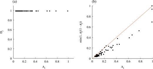
Tecator data: the adaptive parameter |$\eta = (A,D)$| for the exploratory individual adaptation algorithm. (a) Limiting values of the (⁠|$A_j$|⁠, |$D_j$|⁠) pairs align at the top ends of the segments of Fig. 1, with the |$D_j$| close to 1, corresponding to the superefficient setting (ii) of Proposition 1; (b) The attained values of the |$A_{j}$| overestimate the idealized values |${\rm min}\left\{1,{\pi_{j}}/{1-\pi_{j}}\right\}$| of setting (ii) in Proposition 1, indicating low dependence in the posterior.

This example and the previous one show that the simplified posterior (3) is a good fit with many datasets and can indeed be used to guide and design algorithms.

4.3. Performance on problems with very large |$p$|

Bondell & Reich (2012) described a variable selection problem with 22 576 variables and 60 observations on two inbred mouse populations. The covariates are gender and gene expression measurements for 22 575 genes. Three physiological phenotypes are recorded, and used as the response variable in the three datasets: PCR|$i$|⁠, |$i=1,\dots,3$|⁠. We use prior (1) with |$V_{\gamma}=g I$|⁠, where |$g$| is given a half-Cauchy hyperprior distribution, and a hierarchical prior was used for |$\gamma$| by assuming that |$h\sim{\mbox{Be}}\big(1, \frac{p-5}{5}\big)$|⁠, which implies that the prior mean number of included variables is 5. We summarize the results using PCR1, while a more complete analysis of all PCR data is given in the Supplementary Material.

Another dataset, denoted SNP data, relates to genome-wide mapping of a complex trait. The data are weight measurements for 993 outbred mice and 79 748 single nucleotide polymorphisms, SNPs, recorded for each mouse. The testis weight is the response, the body weight is a regressor which is always included in the model and variable selection is performed on the 79 748 SNPs. The high dimensionality makes this a difficult problem and Carbonetto et al. (2017) use a variational inference algorithm, varbvs, for these data. We have used various prior specifications in (1), and present results for a half-Cauchy hyperprior on |$g$| and |$h=5/p$|⁠. Complete results for these data are also provided in the Supplementary Material.

For all datasets, the individual adaptation algorithms were run with |$\tau_{\rm L}=0.05$| and |$\tau_{\rm U}=0.23$|⁠, and |$\tau=0.234$|⁠. The exploratory individual adaptation algorithm had a burn-in of 2150 iterations and 10 750 subsequent iterations and no thinning, and the adaptively scaled individual adaptation had 500 burn-in and 2500 recorded iterations and no thinning, which gave very similar run times. Rao–Blackwellised updates of |$\pi^{(i)}$| were only calculated during the burn-in, and posterior inclusion probability for the |$j$|th variable was estimated by the posterior mean of |$\gamma_j$|⁠. In addition, we show results for the add-delete-swap algorithm and the weighted tempered Gibbs sampler of Zanella & Roberts (2019), which were the most promising alternatives. Three independent runs of all algorithms were executed to gauge the degree of agreement across runs. Using MATLAB and an Intel i7 3.60 GHz processor, each algorithm took about 25 minutes for the PCR data and around 2.5 hours for the SNP data.

Figures 3 and 4 show pairwise comparisons between the different runs for each dataset. The estimates from each independent chain for the adaptively scaled individual adaptation algorithm are very similar, and indicate that the sampler is able to accurately represent the posterior distribution. The weighted tempered Gibbs algorithm performs equally well for the SNP data, but shows worse performance on the PCR1 dataset. The exploratory individual adaptation algorithm does not seem to converge rapidly enough to effectively deal with these very high-dimensional model spaces in the relatively modest running time allocated. Clearly, the add-delete–wap sampler is not able to adequately characterize the posterior model distribution for the PCR data, with dramatically different results across runs, but performs much better for the SNP data.

Fig. 3.

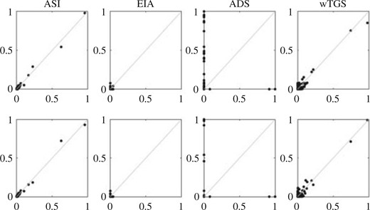
PCR|$1$| data: comparisons of posterior inclusion probabilities from pairs of runs with random |$g$| and |$h$| using adaptively scaled individual adaptation, ASI, exploratory individual adaptation, EIA, add-delete-swap, ADS, and weighted tempered Gibbs sampling, wTGS.

Fig. 4.

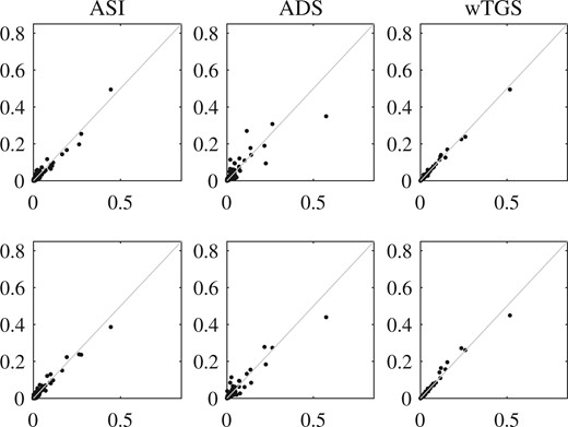
SNP data: comparisons of posterior inclusion probabilities from pairs of runs with random |$g$| and fixed |$h$| using adaptively scaled individual adaptation, ASI, add-delete-swap, ADS, and weighted tempered Gibbs sampling, wTGS.

Acknowledgement

K.Ł. acknowledges support from the Royal Society and the Engineering and Physical Sciences Research Council. The authors thank two referees and an associate editor for their insightful comments that helped improve the paper.

Supplementary material

Supplementary material available at Biometrika online includes proofs, derivations, details of adaptive parallel tempering versions of the algorithms, using the approach of Miasojedow et al. (2013), and further results. Code to run both algorithms is available from https://jimegriffin.github.io/website/.