Semi-exact control functionals from Sard’s method

Summary

A novel control variate technique is proposed for the post-processing of Markov chain Monte Carlo output, based on both Stein’s method and an approach to numerical integration due to Sard. The resulting estimators of posterior expected quantities of interest are proven to be polynomially exact in the Gaussian context, while empirical results suggest that the estimators approximate a Gaussian cubature method near the Bernstein–von Mises limit. The main theoretical result establishes a bias-correction property in settings where the Markov chain does not leave the posterior invariant. Empirical results across a selection of Bayesian inference tasks are presented.

1. Introduction

This paper focuses on the numerical approximation of integrals of the form

$$I(f) = \int f(x) p(x) \,\mathrm{d} x,$$

where |$f$| is a function of interest and |$p$| is a positive and continuously differentiable probability density on |$\mathbb{R}^d$|⁠, under the restriction that |$p$| and its gradient can only be evaluated pointwise up to an intractable normalization constant. The standard approach to computing |$I(f)$| in this context is to simulate the first |$n$| steps of a |$p$|-invariant Markov chain |$(x^{(i)})_{i=1}^\infty$|⁠, possibly after an initial burn-in period, and to take the average along the sample path as an approximation to the integral:

$$\begin{equation}\label{eqn:MC} I(f) \approx I_{\mathrm{MC}}(f) = \frac{1}{n}\sum_{i=1}^n f(x^{(i)}); \end{equation}$$

(1)

see Robert & Casella (2013, Ch. 6–10) for background. In this paper |$\mathbb{E}$|⁠, |$\mathbb{V}$| and |$\mathbb{C}$| respectively denote expectation, variance and covariance with respect to the law |$\mathbb{P}$| of the Markov chain. Under regularity conditions on |$p$| which ensure that the Markov chain |$(x^{(i)})_{i=1}^\infty$| is aperiodic, irreducible and reversible, the convergence of |$I_{\mathrm{MC}}(f)$| to |$I(f)$| as |$n \rightarrow \infty$| is described by a central limit theorem where convergence occurs in distribution and, if the chain starts in stationarity,

$$\begin{equation*} \sigma(f)^2 = \mathbb{V}\{ f(x^{(1)})\} + 2 \sum_{i=2}^\infty \mathbb{C}\{f(x^{(1)}), f(x^{(i)})\} \end{equation*}$$

is the asymptotic variance of |$f$| along the sample path. See Theorem 4.7.7 of Robert & Casella (2013) and more generally Meyn & Tweedie (2012) for theoretical background. For all but the most trivial function |$f$| we have |$\sigma(f)^2 > 0$|⁠, and hence, to achieve an approximation error of |$O_\textrm{P}(\epsilon)$|⁠, a potentially large number |$O(\epsilon^{-2})$| of calls to |$f$| and |$p$| is required.

One approach to reducing this computational cost is to employ control variates (Hammersley & Handscomb, 1964; Ripley, 1987), which involves finding an approximation |$f_n$| to |$f$| that can be exactly integrated under |$p$|⁠, such that |$\sigma(f - f_n)^2 \ll \sigma(f)^2$|⁠. Given a choice of |$f_n$|⁠, the standard estimator (1) is replaced with

$$\begin{equation}\label{eqn:CV} I_{\mathrm{CV}}(f) = \frac{1}{n} \sum_{i=1}^n \{f(x^{(i)}) - f_n(x^{(i)})\} + \underbrace{ \int f_n(x)p(x) \,\mathrm{d}x }_{(*)},\end{equation}$$

(2)

where |$(*)$| is computed exactly. This last requirement makes it challenging to develop control variates for general use, particularly in Bayesian statistics where often the density |$p$| can be accessed only in a form that is unnormalized. In the Bayesian context, Assaraf & Caffarel (1999), Mira et al. (2013) and Oates et al. (2017) addressed this challenge by using |$f_n = c_n + \mathcal{L}g_n$| where |$c_n \in \mathbb{R}$|⁠, |$g_n$| is a user-chosen parametric or nonparametric function and |$\mathcal{L}$| is an operator, such as the Langevin–Stein operator (Stein, 1972; Gorham & Mackey, 2015), that depends on |$p$| through its gradient and satisfies |$\int (\mathcal{L} g_n)(x)p(x) \,\mathrm{d}x = 0$| under regularity conditions; see Lemma 1. Convergence of |$I_{\mathrm{CV}}(f)$| to |$I(f)$| has been studied under strong regularity conditions, and in particular: (i) if |$g_n$| is chosen parametrically, then in general |$\lim\inf \sigma(f - f_n)^2 > 0$| so that even if the asymptotic variance is reduced, convergence rates are unaffected; (ii) if |$g_n$| is chosen in an appropriate nonparametric manner, then |$\lim \sup \sigma(f - f_n)^2 = 0$| and a smaller number |$O(\epsilon^{-2 + \delta})$|⁠, with |$0 < \delta < 2$|⁠, of calls to |$f$|⁠, |$p$| and its gradient is required to achieve an approximation error of |$O_\textrm{P}(\epsilon)$| for the integral (see Mijatović & Vogrinc, 2018; Oates et al., 2019; Belomestny et al., 2020a,b,c; Barp et al., 2021). In the parametric case |$\mathcal{L} g_n$| is called a control variate, while in the nonparametric case it is called a control functional.

Practical parametric approaches to choosing |$g_n$| have been well studied in the Bayesian context, typically based on polynomial regression models (Assaraf & Caffarel, 1999; Mira et al., 2013; Papamarkou et al., 2014; Oates et al., 2016; Brosse et al., 2019), but neural networks have also been proposed recently (Wan et al., 2019; Si et al., 2020). In particular, existing control variates based on polynomial regression have the attractive property of being semi-exact, meaning that there is a well-characterized set of functions |$f \in \mathcal{F}$| for which |$f_n$| can be shown to exactly equal |$f$| after a finite number |$n$| of samples have been obtained. For the control variates of Assaraf & Caffarel (1999) and Mira et al. (2013), the set |$\mathcal{F}$| contains certain low-order polynomials when |$p$| is a Gaussian distribution on |$\mathbb{R}^d$|⁠. Those authors call their control variates zero-variance, but we prefer the term semi-exact since a general integrand |$f$| will not be an element of |$\mathcal{F}$|⁠. Regardless of terminology, semi-exactness of the control variate is an appealing property because it implies that the approximation |$I_{\mathrm{CV}}(f)$| to |$I(f)$| is exact on |$\mathcal{F}$|⁠. Intuitively, the performance of the control variate method is related to the richness of the set |$\mathcal{F}$| on which it is exact. For example, polynomial exactness of cubature rules can be used to establish their high-order convergence rates via a Taylor expansion argument (e.g., Hildebrand, 1987, Ch. 8).

The development of nonparametric approaches to the choice of |$g_n$| has focused on kernel methods (Oates et al., 2017; Barp et al., 2021), piecewise-constant approximations (Mijatović & Vogrinc, 2018) and nonlinear approximations based on selecting basis functions from a dictionary (Belomestny et al., 2020b; South et al., 2020). Theoretical analysis of nonparametric control variates was provided in the papers cited above, but compared with parametric methods, practical implementations of nonparametric methods are less well developed.

In this paper we propose a semi-exact control functional method. This represents the best of both worlds, in that at small |$n$| the semi-exactness property promotes stability and robustness of the estimator |$I_{\mathrm{CV}}(f)$|⁠, while at large |$n$| the nonparametric regression component can be used to accelerate the convergence of |$I_{\mathrm{CV}}(f)$| to |$I(f)$|⁠. In particular, we argue that in the Bernstein–von Mises limit, the set |$\mathcal{F}$| on which our method is exact is precisely the set of low-order polynomials, so that our method can be regarded as an approximately polynomially exact cubature rule developed for the Bayesian context. Furthermore, we establish a bias-correction property, which guarantees that the approximations produced using our method are consistent in certain settings where the Markov chain is not |$p$|-invariant.

Our motivation comes from an approach to numerical integration due to Sard (1949). Many numerical integration methods are based on constructing an approximation |$f_n$| to the integrand |$f$| that can be exactly integrated. In this case the integral |$I(f)$| is approximated using |$(*)$| in (2). In Gaussian and related cubatures, the function |$f_n$| is chosen in such a way that polynomial exactness is guaranteed (Gautschi, 2004, § 1.4). On the other hand, in kernel cubature and related approaches, |$f_n$| is an element of a reproducing kernel Hilbert space chosen such that an error criterion is minimized (Larkin, 1970). The contribution of Sard was to combine these two concepts in numerical integration by choosing |$f_n$| to enforce exactness on a low-dimensional space |$\mathcal{F}$| of functions and using the remaining degrees of freedom to find a minimum-norm interpolant to the integrand.

2. Methods

2.1. Sard’s method

Many popular methods for numerical integration are based on either (i) enforcing exactness of the integral estimator on a finite-dimensional set of functions |$\mathcal{F}$|⁠, typically a linear space of polynomials, or (ii) integration of a minimum-norm interpolant selected from an infinite-dimensional set of functions |$\mathcal{H}$|⁠. In each case, the result is a cubature method of the form

$$\begin{equation} \label{eq:quadrature-generic} I_{\mathrm{NI}}(f) = \sum_{i=1}^n w_i f(x^{(i)})\end{equation}$$

(3)

for weights |$\{w_i\}_{i=1}^n \subset \mathbb{R}$| and points |$\{x^{(i)}\}_{i=1}^n \subset \mathbb{R}^d$|⁠. Classical examples of methods in the former category include univariate Gaussian quadrature rules (Gautschi, 2004, § 1.4), which are determined by the unique |$\{(w_i, x^{(i)})\}_{i=1}^n \subset \mathbb{R} \times \mathbb{R}^d$| such that |$I_{\mathrm{NI}}(f) = I(f)$| whenever |$f$| is a polynomial of order at most |$2n-1$|⁠, and Clenshaw–Curtis rules (Clenshaw & Curtis, 1960). Methods in the minimum-norm interpolant category specify a suitable normed space |$(\mathcal{H}, \|\cdot\|_{\mathcal{H}})$| of functions, construct an interpolant |$f_n \in \mathcal{H}$| such that

$$\begin{equation} \label{eq:minimum-norm} f_n \in \mathop{\mathrm{argmax}}\limits_{ h \in \mathcal{H}} \bigl\{ \|{h}\|_{\mathcal{H}} \, \colon \, h(x^{(i)}) = f(x^{(i)}) \text{ for } i = 1, \ldots, n \bigr\},\end{equation}$$

(4)

and use the integral of |$f_n$| to approximate the true integral. Specific examples include splines (Wahba, 1990) and methods based on kernels or Gaussian processes (Larkin, 1970; O’Hagan, 1991; Briol et al., 2019).

If the set of points |$\{x^{(i)}\}_{i=1}^n$| is fixed, the cubature method in (3) has |$n$| degrees of freedom corresponding to the choice of the weights |$\{w_i\}_{i=1}^n$|⁠. The approach proposed by Sard (1949) is a hybrid of the two classical approaches just described, calling for |$m \leqslant n$| of these degrees of freedom to be used to ensure that |$I_{\mathrm{NI}}(f)$| is exact for |$f$| in a given |$m$|-dimensional linear function space |$\mathcal{F}$| and, if |$m < n$|⁠, allocating the remaining |$n-m$| degrees of freedom to select a minimum-norm interpolant from a large class of functions |$\mathcal{H}$|⁠. The approach of Sard is therefore exact for functions in the finite-dimensional set |$\mathcal{F}$| and, at the same time, suitable for the integration of functions in the infinite-dimensional set |$\mathcal{H}$|⁠. Further background on Sard’s method can be found in Larkin (1974) and Karvonen et al. (2018).

However, it is difficult to implement Sard’s method, or indeed any of the classical approaches just discussed, in the Bayesian context, because:

• (i)

  the density |$p$| can be evaluated pointwise only up to an intractable normalization constant;

• (ii)

  to construct weights, one needs to evaluate the integrals of basis functions of |$\mathcal{F}$| and of the interpolant |$f_n$|⁠, which can be as difficult as evaluating the original integral.

To circumvent these issues, we propose to combine Sard’s approach to integration with Stein operators (Stein, 1972; Gorham & Mackey, 2015), thus eliminating the need to access normalization constants and to exactly evaluate integrals.

2.2. Stein operators

Denote the dot product by |$a \cdot b = a^{ \mathrm{\scriptscriptstyle T} } b$|⁠, the gradient by |$\nabla_{x} = (\partial_{x_1},\dots,\partial_{x_d})^{ \mathrm{\scriptscriptstyle T} }$| and the Laplacian by |$\Delta_{x} = \nabla_{x} \cdot \nabla_{x}$|⁠. Let |$\|x\| = (x \cdot x)^{1/2}$| denote the Euclidean norm on |$\mathbb{R}^d$|⁠. The construction that enables us to realize Sard’s method in the Bayesian context is the Langevin–Stein operator |$\mathcal{L}$| on |$\mathbb{R}^d$| (Gorham & Mackey, 2015), defined for sufficiently regular |$g$| and |$p$| as

$$\begin{align} \label{eq:stein-operator} (\mathcal{L} g)(x) &= \Delta_{x} g(x) + \nabla_{x} g(x) \cdot \nabla_{x} \log{p(x)}.\end{align}$$

(5)

We refer to |$\mathcal{L}$| as a Stein operator owing to the use of equations of the form (5), up to a simple substitution, in the method of Stein (1972) for assessing convergence in distribution and because of its property of producing functions whose integrals with respect to |$p$| are zero under suitable conditions such as those described in Lemma 1.

 

Lemma 1.

If |$g \colon \mathbb{R}^d \rightarrow \mathbb{R}$| is twice continuously differentiable, |$\log p : \mathbb{R}^d \rightarrow \mathbb{R}$| is continuously differentiable and |$\| \nabla_{x} g(x) \| \leqslant C \| x \|^{-\delta} p(x)^{-1}$| is satisfied for some |$C \in \mathbb{R}$| and |$\delta > d -1$|⁠, then

$$\begin{equation*} \int (\mathcal{L} g)(x) p(x) \,\mathrm{d} x=0,\end{equation*}$$

where |$\mathcal{L}$| is the Stein operator in (5).

The proof is provided in the Supplementary Material. Although our attention is limited to (5), the choice of Stein operator is not unique, and other Stein operators can be derived using the generator method of Barbour (1988) or using Schrödinger Hamiltonians (Assaraf & Caffarel, 1999). Contrary to the standard requirements for a Stein operator, the operator |$\mathcal{L}$| in control functionals does not need to fully characterize convergence, and consequently a broader class of functions |$g$| can be considered than in more traditional applications of Stein’s method (Stein, 1972).

It follows that if the conditions of Lemma 1 are satisfied by |$g_n : \mathbb{R}^d \rightarrow \mathbb{R}$|⁠, the integral of a function of the form |$f_n = c_n + \mathcal{L} g_n$| is simply |$c_n$|⁠, the constant. The main challenge in developing control variates, or functionals, based on Stein operators is therefore to find a function |$g_n$| such that the asymptotic variance |$\sigma(f - f_n)^2$| is small. To explicitly minimize asymptotic variance, Mijatović & Vogrinc (2018), Brosse et al. (2019) and Belomestny et al. (2020a) restricted attention to particular Metropolis–Hastings or Langevin samplers for which the asymptotic variance can be explicitly characterized. The minimization of empirical variance has also been proposed and studied in cases where samples are independent (Belomestny et al., 2020b) and dependent (Belomestny et al., 2020a,c). For an approach that is not tied to a particular Markov kernel, Assaraf & Caffarel (1999) and Mira et al. (2013), among others, proposed minimizing the mean squared error along the sample path, which corresponds to the case of an independent sampling method. In a similar spirit, the constructions in Oates et al. (2017, 2019) and Barp et al. (2021) are based on a minimum-norm interpolant, where the choice of norm is decoupled from the mechanism by which the points are sampled.

2.3. The proposed method

In this section we first construct an infinite-dimensional space |$\mathcal{H}$| and a finite-dimensional space |$\mathcal{F}$| of functions; these will underpin the proposed semi-exact control functional method.

For the infinite-dimensional component, let |$k \colon \mathbb{R}^d \times \mathbb{R}^d \to \mathbb{R}$| be a positive-definite kernel, meaning that (i) |$k$| is symmetric, with |$k(x,y) = k(y,x)$| for all |$x,y \in \mathbb{R}^d$|⁠, and (ii) the kernel matrix |$(K)_{i,j} = k(x^{(i)}, x^{(j)})$| is positive definite for any distinct points |$\{ x^{(i)} \}_{i=1}^n \subset \mathbb{R}^d$| and any |$n \in \mathbb{N}$|⁠. Recall that such a |$k$| induces a unique reproducing kernel Hilbert space |$\mathcal{H}(k)$|⁠. This is a Hilbert space consisting of functions |$g \colon \mathbb{R}^d \to \mathbb{R}$| that is equipped with an inner product |$\langle \cdot\,, \cdot \rangle_{\mathcal{H}(k)}$|⁠. The kernel |$k$| is such that |$k(\cdot\,,x) \in \mathcal{H}(k)$| for all |$x \in \mathbb{R}^d$|⁠, and it is reproducing in the sense that |$\langle g, k(\cdot, x) \rangle_{\mathcal{H}(k)} = g(x)$| for any |$g \in \mathcal{H}(k)$| and |$x \in \mathbb{R}^d$|⁠. For |$\alpha \in \mathbb{N}_0^d$| the multi-index notation |$x^{\alpha} = x_1^{\alpha_1} \cdots x_d^{\alpha_d}$| and |$|{\alpha}| = \alpha_1 + \dots + \alpha_d$| will be used. If |$k$| is twice continuously differentiable in the sense of Steinwart & Christmann (2008, Definition 4.35), meaning that the derivatives

$$\begin{equation*} \partial_{x}^{\alpha} \partial_{y}^{\alpha} k(x, y) =\frac{\partial^{2|{\alpha}|}}{\partial x^{\alpha} \partial y^{\alpha}} k(x, y) \end{equation*}$$

exist and are continuous for every multi-index |$\alpha \in \mathbb{N}_0^d$| with |$|{\alpha}| \leqslant 2$|⁠, then

$$\begin{equation} \label{eq:stein-kernel} k_0(x, y) = \mathcal{L}_{x} \mathcal{L}_{y} k(x, y),\end{equation}$$

(6)

where |$\mathcal{L}_{x}$| stands for application of the Stein operator defined in (5) with respect to variable |$x$|⁠, is a well-defined and positive-definite kernel (Steinwart & Christmann, 2008, Lemma 4.34). The kernel in (6) can be written as

$$\begin{equation} \label{eq:stein-kernel2} \begin{split}k_0(x, y) ={}& \Delta_{x} \Delta_{y} k(x, y) + u(x)^{ \mathrm{\scriptscriptstyle T} } \nabla_{x} \Delta_{y} k(x,y) \\ &+ u(y)^{ \mathrm{\scriptscriptstyle T} } \nabla_{y} \Delta_{x} k(x, y) + u(x)^{ \mathrm{\scriptscriptstyle T} } \big\{ \nabla_{x} \nabla_{y}^{ \mathrm{\scriptscriptstyle T} } k(x,y) \big\} u(y), \end{split}\end{equation}$$

(7)

where |$\nabla_{x} \nabla_{y}^{ \mathrm{\scriptscriptstyle T} } k(x, y)$| is the |$d \times d$| matrix with entries |$\{ \nabla_{x} \nabla_{y}^{ \mathrm{\scriptscriptstyle T} } k(x, y)\}_{i,j} = \partial_{x_i} \partial_{y_j} k(x, y)$| and |$u(x) = \nabla_{x} \log p(x)$|⁠. If |$k$| is radial, then (7) can be simplified; see the Supplementary Material. Lemma 2 establishes conditions under which the functions |$x \mapsto k_0(x,y)$|⁠, |$y \in \mathbb{R}^d$|⁠, and hence elements of the Hilbert space |$\mathcal{H}(k_0)$| reproduced by |$k_0$|⁠, have zero integral. Let |$\|M\|_{\mathrm{OP}} = \sup_{\|x\| = 1} \|M x\|$| denote the operator norm of a matrix |$M \in \mathbb{R}^{d \times d}$|⁠.

 

Lemma 2.

If |$k \colon \mathbb{R}^d \times \mathbb{R}^d \rightarrow \mathbb{R}$| is twice continuously differentiable in each argument, |$\log p : \mathbb{R}^d \rightarrow \mathbb{R}$| is continuously differentiable, and |$\| \nabla_{x}\nabla_{y}^{ \mathrm{\scriptscriptstyle T} } k(x,y) \|_{\small{\text{OP}}} \leqslant C(y) \| x \|^{-\delta} p(x)^{-1}$| and |$\| \nabla_{x}\Delta_{y}k(x,y) \| \leqslant C(y) \| x \|^{-\delta} p(x)^{-1}$| are satisfied for some |$C: \mathbb{R}^d \rightarrow (0,\infty)$| and |$\delta > d -1$|⁠, then

$$\begin{equation} \label{eq: kernel ints to 0} \int k_0(x, y) p(x) {\rm d} x = 0\end{equation}$$

(8)

for every |$y \in \mathbb{R}^d$|⁠, where |$k_0$| is defined in (6).

The proof is provided in the Supplementary Material. The infinite-dimensional space |$\mathcal{H}$| used here is exactly the reproducing kernel Hilbert space |$\mathcal{H}(k_0)$|⁠. The basic mathematical properties of |$k_0$| and the Hilbert space it reproduces are given in the Supplementary Material, and these can be used to inform the selection of an appropriate kernel.

For the finite-dimensional component, let |$\Phi$| be a linear space of twice continuously differentiable functions with dimension |$m-1$|⁠, where |$m \in \mathbb{N}$|⁠, and a basis |$\{\phi_i\}_{i=1}^{m-1}$|⁠. Define the space obtained by applying the differential operator (5) to |$\Phi$| as |$\mathcal{L} \Phi = \mathrm{span}\{ \mathcal{L} \phi_1, \ldots, \mathcal{L} \phi_{m-1} \}$|⁠. If the preconditions of Lemma 1 are satisfied for each basis function |$g = \phi_i$|⁠, then linearity of the Stein operator implies that |$\int (\mathcal{L}\phi) \,\mathrm{d}p = 0$| for every |$\phi \in \Phi$|⁠. Typically we will select |$\Phi = \mathcal{P}^r$| as the polynomial space |$\mathcal{P}^r = \mathrm{span} \{ x^{\alpha} : \alpha \in \mathbb{N}_0^d, \, 0 < |{\alpha}| \leqslant r \}$| for some nonnegative integer |$r$|⁠. Constant functions are excluded from |$\mathcal{P}^r$| since they are in the null space of |$\mathcal{L}$|⁠; when required we let |$\mathcal{P}_0^r = \text{span}\{1\} \oplus \mathcal{P}^r$| denote the larger space with the constant functions included. The finite-dimensional space |$\mathcal{F}$| is then taken to be |$ \mathcal{F} = \mathrm{span} \{1\} \oplus \mathcal{L} \Phi = \mathrm{span} \{1, \mathcal{L} \phi_1, \ldots \mathcal{L} \phi_{m-1} \}$|⁠.

We are now ready to state the proposed method. Following Sard, we approximate the integrand |$f$| with a function |$f_n$| that interpolates |$f$| at the locations |$x^{(i)}$|⁠, is exact on the |$m$|-dimensional linear space |$\mathcal{F}$|⁠, and minimizes a particular seminorm subject to the first two constraints. It will occasionally be useful to emphasize the dependence of |$f_n$| on |$f$| using the notation |$f_n(\cdot) = f_n(\cdot\, ; f)$|⁠. The proposed interpolant takes the form

$$\begin{equation} \label{eq:interpolant} f_n(x) = b_1 + \sum_{i=1}^{m-1} b_{i+1} (\mathcal{L} \phi_i) (x) + \sum_{i=1}^n a_i k_0(x, x^{(i)}),\end{equation}$$

(9)

where the coefficients |$a = (a_1,\ldots,a_n) \in \mathbb{R}^n$| and |$b = (b_1,\ldots,b_m) \in \mathbb{R}^m$| are selected such that the following two conditions hold.

 

Condition 1

(Interpolation). We have |$f_n(x^{(i)} ; f) = f(x^{(i)})$| for |$i = 1, \ldots, n$|⁠.

 

Condition 2

(Semi-exactness) We have |$f_n(\cdot\, ;f) = f(\cdot)$| whenever |$f \in \mathcal{F}$|⁠.

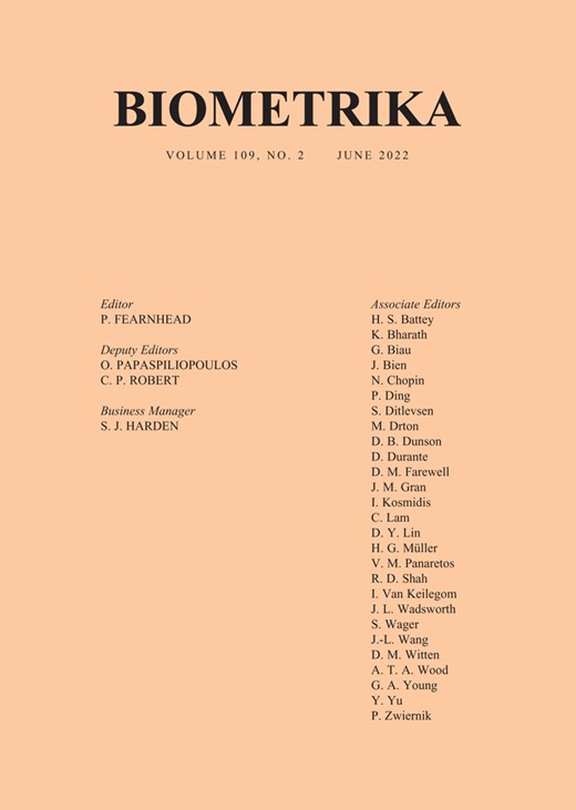
Since |$\mathcal{F}$| is |$m$|-dimensional, these requirements yield a total of |$n+m$| constraints. Under weak conditions, discussed in § 2.5, the total number of degrees of freedom due to selection of |$a$| and |$b$| is equal to |$n+m$| and Conditions 1 and 2 can be satisfied. Furthermore, the corresponding function |$f_n$| can be shown to minimize a particular seminorm on a larger space of functions, subject to the interpolation and exactness constraints; to limit the scope of the paper, we do not discuss this characterization further, but the seminorm is defined in (16) and the reader can find full details in Wendland (2004, Theorem 13.1). Figure 1 illustrates one such interpolant. The proposed estimator of the integral is then

Fig. 1.

(a) The interpolant |$f_n$| from (9) at |$n=5$| points to the function |$f(x) = \sin\{0.5\pi (x-1)\} + \exp\{-(x-0.5)^2\}$| for the Gaussian density |$p(x) = \mathcal{N}(x; 0,1)$|⁠; the interpolant uses the Gaussian kernel |$k(x,y) = \exp\{-(x-y)^2\}$| and a polynomial parametric basis with |$r=2$|⁠. Two translates (b) |$k_0(\cdot\,,0)$| and (c) |$k_0(\cdot\,,1)$| of the kernel (6).

$$\begin{equation} \label{eq:BSS-def} I_{\mathrm{SECF}}(f) = \int f_n(x) p(x) {\rm d} x,\end{equation}$$

(10)

a special case of (2) that we call a semi-exact control functional, as the interpolation condition causes the first term in (2) to vanish. The following is immediate from (9) and (10).

 

Corollary 1.

Under the hypotheses of Lemma 1 for each |$g = \phi_i \ (i = 1,\dots,m-1)$| and Lemma 2, whenever the estimator |$I_{\mathrm{SECF}}(f)$| is well-defined, we have |$I_{\mathrm{SECF}}(f) = b_1$| where |$b_1$| is the constant term in (9).

The earlier work of Assaraf & Caffarel (1999) and Mira et al. (2013) corresponds to |$a = 0$| and |$b \neq 0$|⁠, while setting |$b = 0$| in (9) and ignoring the semi-exactness requirement recovers the unique minimum-norm interpolant in the Hilbert space |$\mathcal{H}(k_0)$| where |$k_0$| is reproducing, in the sense of (4). The work of Oates et al. (2017) corresponds to |$b_i = 0$| for |$i = 2,\dots,m$|⁠. It is therefore clear that the proposed approach is a strict generalization of existing work and can be seen as a compromise between semi-exactness and minimum-norm interpolation.

2.4. Polynomial exactness in the Bernstein–von Mises limit

A central motivation for our approach is the prototypical case where |$p$| is the density of a posterior distribution |$P_{x \mid y_1,\dots,y_N}$| for a latent variable |$x$| given independent and identically distributed data |$y_1,\dots,y_N \sim P_{y_1,\dots,y_N \mid x}$|⁠. Under regularity conditions discussed in van der Vaart (1998, § 10.2), the Bernstein–von Mises theorem states that

$$\begin{equation*} \big\| P_{x \mid y_1,\dots,y_N} - \mathcal{N}\{\hat{x}_N, N^{-1} I(\hat{x}_N)^{-1}\} \big\|_{\mathrm{TV}} \rightarrow 0,\end{equation*}$$

where |$\hat{x}_N$| is a maximum likelihood estimate for |$x$|⁠, |$I(x)$| is the Fisher information matrix evaluated at |$x$|⁠, |$\|\cdot\|_{\mathrm{TV}}$| is the total variation norm, and convergence is in probability as |$N \rightarrow \infty$| with respect to the law |$P_{y_1,\dots,y_N \mid x}$| of the dataset. In this limit, polynomial exactness of the proposed method can be established. Indeed, for a Gaussian density |$p$| with mean |$\hat{x}_N \in \mathbb{R}^d$| and precision |$N I(\hat{x}_N)$|⁠, if |$\phi(x) = x^{\alpha}$| for a multi-index |$\alpha \in \mathbb{N}_0^d$|⁠, then

$$\begin{equation*} (\mathcal{L} \phi)(x) = \sum_{i=1}^d \alpha_i\left\{ (\alpha_i-1) x_i^{\alpha_i-2} -\frac{N}{2} P_i(x) x_i^{\alpha_i-1} \right\} \prod_{j \neq i} x_j^{\alpha_j},\end{equation*}$$

where |$P_i(x) = 2e_i^{ \mathrm{\scriptscriptstyle T} } I(\hat{x}_N) (x - \hat{x}_N)$| with |$e_i$| being the |$i$|th coordinate vector in |$\mathbb{R}^d$|⁠. This allows us to obtain the following result, whose proof is provided in the Supplementary Material.

 

Lemma 3.

Consider the Bernstein–von Mises limit and suppose that the Fisher information matrix |$I(\hat{x}_N)$| is nonsingular. Then, for the choice |$\Phi = \mathcal{P}^r$| with |$r \in \mathbb{N}$|⁠, the estimator |$I_\mathrm{SECF}$| is exact on |$\mathcal{F} = \mathcal{P}_0^r$|⁠.

Thus the proposed estimator is polynomially exact up to order |$r$| in the Bernstein–von Mises limit. We believe that this property can confer robustness of the estimator in a broad range of applied contexts. At finite |$N$|⁠, when the limit has not been reached, the above argument can be expected to hold only approximately.

2.5. Computation for the proposed method

Define the |$n \times m$| matrix

$$\begin{equation} P = \begin{pmatrix} 1 \; & \mathcal{L} \phi_1(x^{(1)}) & \cdots & \mathcal{L} \phi_{m-1}(x^{(1)}) \\ \vdots & \vdots & \ddots & \vdots \\ 1 \; & \mathcal{L} \phi_1 (x^{(n)}) & \cdots & \mathcal{L} \phi_{m-1}( x^{(n)}) \end{pmatrix}, \label{eq: def for P}\end{equation}$$

(11)

which is sometimes called a Vandermonde or alternant matrix, corresponding to the linear space |$\mathcal{F}$|⁠. Let |$K_0$| be the |$n \times n$| matrix with entries |$(K_0)_{i,j} = k_0(x^{(i)}, x^{(j)})$|⁠, and let |$f$| be the |$n$|-dimensional column vector with entries |$(f)_i = f(x^{(i)})$|⁠.

 

Lemma 4.

Let the |$n \geqslant m$| points |$x^{(i)}$| be distinct and |$\mathcal{F}$|-unisolvent, meaning that the matrix |$P$| in (11) has full rank. Let |$k_0$| be a positive-definite kernel for which (8) is satisfied. Then |$I_{\mathrm{SECF}}(f)$| is well-defined and the coefficients |$a$| and |$b$| are given by the solution of the linear system

$$\begin{equation} \label{eq:block-system} \begin{pmatrix} K_0 & P \\ P^{ \mathrm{\scriptscriptstyle T} } & 0 \end{pmatrix} \begin{pmatrix} a \\ b \end{pmatrix} = \begin{pmatrix} f \\ 0 \end{pmatrix}.\end{equation}$$

(12)

In particular,

$$\begin{equation}\label{eqn:BSS} I_{\mathrm{SECF}}(f) = e_1^{ \mathrm{\scriptscriptstyle T} } ( P^{ \mathrm{\scriptscriptstyle T} } K_0^{-1} P )^{-1} P^{ \mathrm{\scriptscriptstyle T} } K_0^{-1} f.\end{equation}$$

(13)

The proof is provided in the Supplementary Material. Equation (13) is a linear combination of the values in |$f$| and so the proposed estimator can be recognized as a cubature method of the form (3) with weights

$$\begin{equation} \label{eq: weights} w = K_0^{-1} P ( P^{ \mathrm{\scriptscriptstyle T} } K_0^{-1} P )^{-1} e_1.\end{equation}$$

(14)

The requirement in Lemma 4 for the |$x^{(i)}$| to be distinct precludes, for example, the direct use of Metropolis–Hastings output. However, as emphasized in Oates et al. (2017) for control functionals and studied further in Liu & Lee (2017) and Hodgkinson et al. (2020), the consistency of |$I_{\mathrm{SECF}}$| does not require that the Markov chain be |$p$|-invariant. It is therefore trivial to, for example, filter out duplicate states from Metropolis–Hastings output.

The solution of linear systems of equations defined by an |$n \times n$| matrix |$K_0$| and an |$m \times m$| matrix |$P^{ \mathrm{\scriptscriptstyle T} } K_0^{-1} P$| entails a computational cost of |$O(n^3 + m^3)$|⁠. In some situations this cost may yet be smaller than the cost associated with evaluation of |$f$| and |$p$|⁠, but in general this computational requirement limits the applicability of the method just described. In the Supplementary Material we propose a computationally efficient approximation, |$I_{\mathrm{ASECF}}$|⁠, to the full method, based on a combination of the Nyström approximation (Williams & Seeger, 2001) and the well-known conjugate gradient method, inspired by the recent work of Rudi et al. (2017).

3. Empirical assessment

3.1. Experimental set-up

We performed a detailed comparison of existing and proposed control variate and control functional techniques. Three examples were considered: a Gaussian target, representing the Bernstein–von Mises limit; a setting in which nonparametric control functional methods perform well; and a setting where parametric control variate methods are known to be successful. In each case we determine whether or not the proposed semi-exact control functional method is competitive with the state-of-the-art technique.

Specifically, we compare the following estimators, all instances of |$I_{\mathrm{CV}}$| in (2) for a particular choice of |$f_n$|⁠, which may or may not be an interpolant:

• (i)

  standard Monte Carlo integration, (1), based on Markov chain output;

• (ii)

  the control functional estimator recommended in Oates et al. (2017), |$I_{\mathrm{CF}}(f) = (1^{ \mathrm{\scriptscriptstyle T} }K_0^{-1}1)^{-1} 1^{{ \mathrm{\scriptscriptstyle T} }} K_0^{-1}f$|⁠;

• (iii)

  the zero-variance polynomial control variate method of Assaraf & Caffarel (1999) and Mira et al. (2013), |$I_{\mathrm{ZV}}(f) = e_1^{ \mathrm{\scriptscriptstyle T} } (P^{ \mathrm{\scriptscriptstyle T} } P)^{-1}P^{ \mathrm{\scriptscriptstyle T} } f$|⁠;

• (iv)

  the auto-zero-variance approach of South et al. (2020), which uses five-fold cross-validation to automatically select (A) between the ordinary least squares solution |$I_{\mathrm{ZV}}$| and an |$\ell_1$|-penalized alternative, where the penalization strength is itself selected using 10-fold cross-validation within the test dataset, and (B) the polynomial order;

• (v)

  the proposed semi-exact control functional estimator, (13);

• (vi)

  an approximation, |$I_{\mathrm{ASECF}}$|⁠, of (13) based on the Nyström approximation and the conjugate gradient method, described in the Supplementary Material.

Open-source software for implementing all of the above methods is available in the |$\texttt{R}$| (R Development Core Team, 2022) package |$\texttt{ZVCV}$| (South, 2020). The same sets of |$n$| samples were used for all estimators, in both the construction of |$f_n$| and the evaluation of |$I_{\mathrm{CV}}$|⁠. For methods in which there is a fixed polynomial basis we considered only orders |$r=1$| and |$r=2$|⁠, following the recommendation of Mira et al. (2013). For kernel-based methods, duplicate values of |$x_i$| were removed, as discussed in § 2.5, and Frobenius regularization was employed whenever the condition number of the kernel matrix |$K_0$| was close to machine precision (Higham, 1988). Several choices of kernel were considered, but for brevity we focus here on the rational quadratic kernel |$k(x,y; \lambda) = (1+\lambda^{-2} \|x-y\|^2)^{-1}$|⁠. This kernel was found to yield the best performance across a range of experiments; a comparison with the Matérn and Gaussian kernels is provided in the Supplementary Material. The parameter |$\lambda$| was selected using five-fold cross-validation, based again on performance across a spectrum of experiments; a comparison with the median heuristic (Garreau et al., 2017) is presented in the Supplementary Material.

To ensure that our assessment is practically relevant, the estimators were compared on the basis of both statistical and computational efficiency relative to the standard Monte Carlo estimator. The statistical efficiency |$\mathcal{E}(I_\text{CV})$| and computational efficiency |$\mathcal{C}(I_\text{CV})$| of an estimator |$I_\text{CV}$| of the integral |$I$| are defined as

$$\begin{eqnarray*} \mathcal{E}(I_\text{CV}) = \frac{\mathbb{E}\{ (I_{\mathrm{MC}} - I)^2 \} }{\mathbb{E}\{ (I_\text{CV} - I)^2 \} }, \quad \mathcal{C}(I_\text{CV}) = \mathcal{E}(I_\text{CV}) \frac{T_{\mathrm{MC}}}{T_\text{CV}},\end{eqnarray*}$$

where |$T_\text{CV}$| denotes the combined wall time for sampling the |$x^{(i)}$| and computing the estimator |$I_\text{CV}$|⁠. For the results reported below, |$\mathcal{E}$| and |$\mathcal{C}$| were approximated using averages |$\hat{\mathcal{E}}$| and |$\hat{\mathcal{C}}$| over 100 realizations of the Markov chain output.

3.2. Gaussian illustration

Here we consider a Gaussian integral that serves as an analytically tractable caricature of a posterior near the Bernstein–von Mises limit. This enables us to assess the effect of the sample size |$n$| and dimension |$d$| on each estimator, in a setting that is not confounded by the idiosyncrasies of any particular Markov chain Monte Carlo method. Specifically, we set |$p(x) = (2\pi)^{-d/2} \exp(-\|x\|^2 / 2)$| where |$x \in \mathbb{R}^d$|⁠. For the parametric component we set |$\Phi = \mathcal{P}^r$| so that, from Lemma 3, |$I_{\mathrm{SECF}}$| is exact on polynomials of order at most |$r$|⁠; this holds also for |$I_{\mathrm{ZV}}$|⁠. For the integrand |$f : \mathbb{R}^d \rightarrow \mathbb{R}$| with |$d \geqslant 3$|⁠, we took

$$\begin{equation}\label{eqn:Gaussian_combin} f(x) = 1 + x_2 + 0.1 x_1 x_2 x_3 + \sin(x_1) \exp\{-(x_2 x_3)^2\}\end{equation}$$

(15)

so that the integral is analytically tractable, i.e., |$I(f) = 1$|⁠, and no method will be exact.

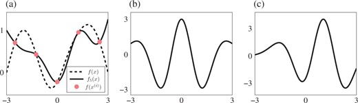
Figure 2 displays the statistical efficiency of each estimator for |$10 \leqslant n \leqslant 1000$| and |$3 \leqslant d \leqslant 100$|⁠. Computational efficiency is not shown since exact sampling from |$p$| in this example is trivial. The proposed semi-exact control functional method performs consistently well compared to its competitors for this nonpolynomial integrand. Unsurprisingly, the best improvements are for large |$n$| and small |$d$|⁠, where the proposed method results in a statistical efficiency over 100 times better than the baseline estimator and up to five times better than the next-best method.

Fig. 2.

Gaussian example: (a) estimated statistical efficiency |$\hat{\mathcal{E}}$| with |$d=4$| and (b) estimated statistical efficiency |$\hat{\mathcal{E}}$| with |$n=1000$| for the integrand (15). The methods compared are standard Monte Carlo integration (light blue), the control functional estimator of Oates et al. (2017) (dark blue), the zero-variance polynomial control variate method of Assaraf & Caffarel (1999) and Mira et al. (2013) (green), the auto-zero-variance approach of South et al. (2020) (yellow), the proposed semi-exact control functional estimator (orange), and an approximate semi-exact control functional estimator (pink); dashed and solid lines correspond to polynomial order 2 and order 1, respectively (if applicable).

3.3. Capture-recapture example

The two remaining examples, presented here and in § 3.4, are applications of Bayesian statistics described in South et al. (2020). In each case the aim is to estimate expectations with respect to a posterior distribution |$P_{x \mid y}$| of the parameters |$x$| of a statistical model based on |$y$|⁠, an observed dataset. Samples |$x^{(i)}$| were obtained using the Metropolis-adjusted Langevin algorithm (Roberts & Tweedie, 1996), which is a Metropolis–Hastings algorithm with proposal |$\mathcal{N} \{ x^{(i-1)} + (h^2/2)\Sigma\nabla_{x} \log P_{x \mid y}(x^{(i-1)} \mid y), h^2 \Sigma\}$|⁠. Step sizes of |$h=0.72$| for the capture-recapture example and |$h=0.3$| for the sonar example in § 3.4 were selected, and an empirical approximation of the posterior covariance matrix was used as the preconditioner |$\Sigma \in \mathbb{R}^{d\times d}$|⁠. Since the proposed method does not rely on the Markov chain being |$P_{x \mid y}$|-invariant, we also repeated these experiments using the unadjusted Langevin algorithm (Ermak, 1975; Parisi, 1981); the results are similar and are reported in the Supplementary Material.

In this first example, a Cormack–Jolly–Seber capture-recapture model (Lebreton et al., 1992) is used to model data on the capture and recapture of the bird species Cinclus cinclus (Marzolin, 1988). The integrands of interest are the marginal posterior means |$f_i(x) = x_i$||$(i=1,\ldots,11)$|⁠, where |$x=(\phi_1,\ldots,\phi_5,p_2,\ldots,p_6,\phi_6 p_7)$|⁠, with |$\phi_j$| the probability of survival from year |$j$| to |$j+1$| and |$p_j$| the probability of being captured in year |$j$|⁠. The likelihood is

$$\begin{align*} \ell(y\mid x) \propto \prod_{i=1}^{6}\chi_i^{d_i} \prod_{k=i+1}^{7} \biggl\{ \phi_i p_k \prod_{m=i+1}^{k-1} \phi_m (1-p_m) \biggr\}^{y_{ik}},\end{align*}$$

where |$d_i=D_i-\sum_{k=i+1}^{7}y_{ik}$|⁠, |$\chi_i=1-\sum_{k=i+1}^{7} \phi_i p_k \prod_{m=i+1}^{k-1} \phi_m (1-p_m)$| and the data |$y$| consist of |$D_i$|⁠, the number of birds released in year |$i$|⁠, and |$y_{ik}$|⁠, the number of birds caught in year |$k$| out of those released in year |$i$|⁠, for |$i=1,\ldots,6$| and |$k=2,\ldots,7$|⁠. Following South et al. (2020), parameters are transformed to the real line using |$\tilde{x}_j=\log\{x_j/(1-x_j)\}$| and the adjusted prior density for |$\tilde{x}_j$| is |$\exp(\tilde{x}_j)/\{1+\exp(\tilde{x}_j)\}^2$||$(j=1,\ldots,11)$|⁠.

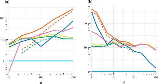
South et al. (2020) found that nonparametric methods outperformed standard parametric methods for this 11-dimensional example. The estimator |$I_{\mathrm{SECF}}$| combines elements of both approaches, so one is interested in determining how the method performs. It is clear from Fig. 3 that all variance-reduction approaches are helpful in improving upon the vanilla Monte Carlo estimator in this example. The best improvement in terms of statistical and computational efficiency is provided by |$I_{\mathrm{SECF}}$|⁠, which also has similar performance to |$I_{\mathrm{CF}}$|⁠.

Fig. 3.

Capture-recapture example: (a) estimated statistical efficiency |$\hat{\mathcal{E}}$| and (b) estimated computational efficiency |$\hat{\mathcal{C}}$|⁠. Efficiency here is reported as an average over the 11 expectations of interest. The methods compared are standard Monte Carlo integration (light blue), the control functional estimator of Oates et al. (2017) (dark blue), the zero-variance polynomial control variate method of Assaraf & Caffarel (1999) and Mira et al. (2013) (green), the auto-zero-variance approach of South et al. (2020) (yellow), the proposed semi-exact control functional estimator (orange), and an approximate semi-exact control functional estimator (pink); dashed and solid lines correspond to polynomial order 2 and order 1, respectively (if applicable).

3.4. Sonar example

Our final application is a 61-dimensional logistic regression example using data from Gorman & Sejnowski (1988) and Dheeru & Karra Taniskidou (2017). In standard regression notation, the parameters are denoted by |$\beta \in \mathbb{R}^{61}$|⁠, the matrix of covariates in the logistic regression model is |$X \in \mathbb{R}^{208 \times 61}$|⁠, where the first column consists of all ones to fit an intercept, and the response is denoted by |$y \in \mathbb{R}^{208}$|⁠. In this application, |$X$| contains information related to energy frequencies reflected from either a metal cylinder, |$y=1$|⁠, or a rock, |$y=0$|⁠. The loglikelihood for this model is

$$\begin{equation*}\label{eqn:logistic}\log \ell(y,X\mid \beta) = \sum_{i=1}^{208} \big[y_i X_{i,\cdot}\beta - \log \{1+\exp(X_{i,\cdot}\beta) \}\big].\end{equation*}$$

We use an |$\mathcal{N}(0,5^2)$| prior for the predictors, after standardizing to a standard deviation of 0.5, and a |$\mathcal{N}(0,20^2)$| prior for the intercept, following Chopin & Ridgway (2017) and South et al. (2020); however, we focus on estimating the more challenging integrand |$f(\beta) = \{ 1+\exp(-\tilde{X}\beta) \}^{-1}$|⁠, which can be interpreted as the probability that observed covariates |$\tilde{X}$| emanate from a metal cylinder. The gold standard of |$I \approx 0.4971$| was obtained from a Metropolis–Hastings procedure (Hastings, 1970) with 10 million iterations, run with a multivariate normal random walk proposal.

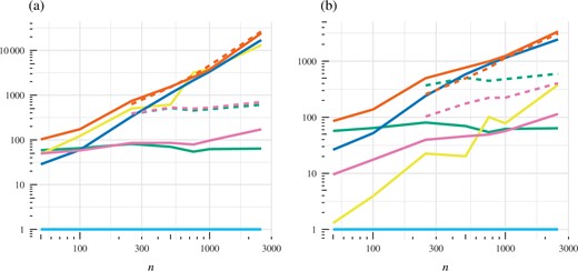
Figure 4 illustrates the statistical and computational efficiency of estimators for various |$n$| in this example. It is interesting that |$I_{\mathrm{SECF}}$| and |$I_{\mathrm{ASECF}}$| offer similar statistical efficiency to |$I_{\mathrm{ZV}}$|⁠, especially given the poor relative performance of |$I_{\mathrm{CF}}$|⁠. Since it is inexpensive to obtain the |$n$| samples using the Metropolis-adjusted Langevin algorithm in this example, |$I_{\mathrm{ZV}}$| and |$I_{\mathrm{ASECF}}$| are the only approaches that yield improvements in computational efficiency over the baseline estimator for the majority of |$n$| values considered, and even in these instances the improvements are marginal.

Fig. 4.

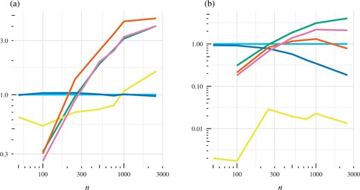
Sonar example: (a) estimated statistical efficiency |$\hat{\mathcal{E}}$| and (b) estimated computational efficiency |$\hat{\mathcal{C}}$|⁠. The methods compared are standard Monte Carlo integration (light blue), the control functional estimator of Oates et al. (2017) (dark blue), the zero-variance polynomial control variate method of Assaraf & Caffarel (1999) and Mira et al. (2013) (green), the auto-zero-variance approach of South et al. (2020) (yellow), the proposed semi-exact control functional estimator (orange), and an approximate semi-exact control functional estimator (pink).

4. Theoretical properties and convergence assessment

4.1. Finite-sample error and a practical diagnostic

The performance of the proposed method can be monitored using the finite-sample error bound provided in Proposition 1. Proposition 1 makes use of the seminorm

$$\begin{align}|f|_{k_0,\mathcal{F}} = \inf_{\substack{f = h + g, \\ h \in \mathcal{F}, \, g \in \mathcal{H}(k_0) }} \|g\|_{\mathcal{H}(k_0)}, \label{eq: semi norm mt}\end{align}$$

(16)

which is well-defined when the infimum is taken over a nonempty set; otherwise |$|f|_{k_0,\mathcal{F}} = \infty$|⁠.

 

Proposition 1.

Suppose that the hypotheses of Corollary 1 hold. Then the integration error satisfies the bound

$$\begin{equation}\lvert I(f) - I_{\mathrm{SECF}}(f) \rvert \leqslant |f|_{k_0,\mathcal{F}} \, (w^{ \mathrm{\scriptscriptstyle T} } K_0 w)^{1/2}, \label{eq: error bound KSD}\end{equation}$$

(17)

where the weights |$w$|⁠, defined in (14), satisfy

$$\begin{equation*}w = arg\,min_{ v \in \mathbb{R}^n} (v^{ \mathrm{\scriptscriptstyle T} } K_0 v)^{1/2} ~~\text{such that}~~ \sum_{i=1}^n v_i h(x^{(i)}) = \int h(x) p(x) {\rm d} x ~~\text{for every } h \in \mathcal{F}.\end{equation*}$$

The proof is provided in the Supplementary Material. The first quantity on the right-hand side of (17), |$|f|_{k_0,\mathcal{F}}$|⁠, can be approximated by |$|f_n|_{k_0,\mathcal{F}}$| when |$f_n$| is a reasonable approximation for |$f$|⁠, and this can in turn can be bounded as |$|f_n|_{k_0,\mathcal{F}} \leqslant (a^{ \mathrm{\scriptscriptstyle T} } K_0 a)^{1/2}$|⁠. The finiteness of |$|f|_{k_0,\mathcal{F}}$| ensures the existence of a solution to the Stein equation, sufficient conditions for which are discussed in Mackey & Gorham (2016) and Si et al. (2020). The second quantity on the right-hand side of (17), |$(w^{ \mathrm{\scriptscriptstyle T} } K_0 w)^{1/2}$|⁠, is computable and can be recognized as a kernel Stein discrepancy between the empirical measure |$\sum_{i=1}^n w_i \delta(x^{(i)})$| and the distribution whose density is |$p$|⁠, based on the Stein operator |$\mathcal{L}$| (Chwialkowski et al., 2016; Liu et al., 2016). Our choice of Stein operator differs from that in Chwialkowski et al. (2016) and Liu et al. (2016). There has been substantial recent research into the use of kernel Stein discrepancies for assessing algorithm performance in the Bayesian computational context (Gorham & Mackey, 2017; Chen et al., 2018, 2019; Singhal et al., 2020; Hodgkinson et al., 2020), and one can also exploit this discrepancy as a diagnostic for the performance of the semi-exact control functional. The diagnostic that we propose to monitor is the product |$(w^{ \mathrm{\scriptscriptstyle T} } K_0 w)^{1/2} (a^{ \mathrm{\scriptscriptstyle T} } K_0 a)^{1/2}$|⁠. This approach to error estimation was also suggested, outside the Bayesian context, in Fasshauer (2011, § 5.1).

The empirical results shown in Fig. 5 suggest that this diagnostic provides a conservative approximation of the actual error. Further work is needed to establish whether this diagnostic detects convergence and nonconvergence in general.

Fig. 5.

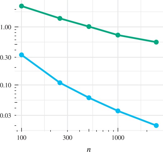
The mean absolute error (blue) and mean of the approximate upper bound |$(w^{ \mathrm{\scriptscriptstyle T} } K_0 w)^{1/2} (a^{ \mathrm{\scriptscriptstyle T} } K_0 a)^{1/2}$| (green) for different values of |$n$| in the sonar example of § 3.4. Both are based on the semi-exact control functional method with |$\Phi = \mathcal{P}^1$|⁠.

4.2. Consistency of the estimator

In what follows we consider an increasing number |$n$| of samples |$\boldsymbol{x}^{(i)}$|⁠, while the finite-dimensional space |$\Phi$|⁠, with basis |$\{\phi_1,\dots,\phi_{m-1}\}$|⁠, is held fixed. The samples |$\boldsymbol{x}^{(i)}$| will be assumed to arise from a |$V$|-uniformly ergodic Markov chain; the reader is referred to Meyn & Tweedie (2012, Ch. 16) for the relevant background. Recall that the points |$(x^{(i)})_{i=1}^n$| are said to be |$\mathcal{F}$|-unisolvent if the matrix in (11) has full rank. It will be convenient to introduce an inner product |$\langle {u}, {v} \rangle_n = {u}^{ \mathrm{\scriptscriptstyle T} } {K}_0^{-1} {v}$| and associated norm |$\|{u}\|_n = \langle {u}, {u} \rangle_n^{1/2}$|⁠. Let |$\Pi$| be the matrix that projects orthogonally onto the columns of |$[{\Psi}]_{i,j} = \mathcal{L} \phi_j({x}^{(i)})$| with respect to the |$\langle \cdot \,, \cdot \rangle_n$| inner product.

 

Theorem 1.

Suppose that the hypotheses of Corollary 1 hold, and let |$f$| be any function for which |$|f|_{k_0,\mathcal{F}} < \infty$|⁠. Let |$q$| be a probability density with |$p/q > 0$| on |$\mathbb{R}^d$|⁠, and consider a |$q$|-invariant Markov chain |$({x}^{(i)})_{i=1}^n$|⁠, assumed to be |$V$|-uniformly ergodic for some |$V : \mathbb{R}^d \rightarrow [1,\infty)$|⁠, such that

• (i)

  |$\sup_{x \in \mathbb{R}^d} \; V(x)^{-r} \; \{p(\boldsymbol{x}) / q(\boldsymbol{x})\}^4 \; k_0(x,x)^2 < \infty$| for some |$0 < r < 1$|⁠;

• (ii)

  the points |$(x^{(i)})_{i=1}^n$| are almost surely distinct and |$\mathcal{F}$|-unisolvent;

• (iii)

  |$\lim\sup_{n \rightarrow \infty} \| \Pi \,{1} \|_n / \| {1} \|_n < 1$| almost surely.

Then |$| I_{\mathrm{SECF}}(f) - I(f)| = O_\mathrm{P}(n^{1/2})$|⁠.

This demonstrates that, even in the biased-sampling setting, the proposed estimator is consistent. The proof is provided in the Supplementary Material and exploits a recent theoretical contribution from Hodgkinson et al. (2020). Assumption (i) serves to ensure that |$q$| is similar enough to |$p$| that a |$q$|-invariant Markov chain will also explore the high-probability regions of |$p$|⁠, as discussed in Hodgkinson et al. (2020). Sufficient conditions for |$V$|-uniform ergodicity are necessarily Markov chain-dependent. The case of the Metropolis-adjusted Langevin algorithm is discussed in Roberts & Tweedie (1996) and Chen et al. (2019), and in particular Theorem 9 of Chen et al. (2019) gives sufficient conditions for |$V$|-uniform ergodicity with |$V(\boldsymbol{x}) = \exp(s \|\boldsymbol{x}\|)$| for all |$s > 0$|⁠. Under these conditions, and with the rational quadratic kernel |$k$| considered in § 3, we have |$k_0(\boldsymbol{x},\boldsymbol{x}) = O\{\|\nabla_{\boldsymbol{x}} \log p(\boldsymbol{x})\|^2\}$| and so (i) is satisfied whenever |$\{p(\boldsymbol{x}) / q(\boldsymbol{x}) \} \|\nabla_{\boldsymbol{x}} \log p(\boldsymbol{x})\| = O\{\exp( t \|\boldsymbol{x}\|)\}$| for some |$t > 0$|⁠, a weak requirement. Assumption (ii) ensures that the finite-sample error bound (17) is almost surely well-defined. Assumption (iii) ensures that the points in the sequence |$(\boldsymbol{x}^{(i)})_{i=1}^n$| distinguish, asymptotically, the constant function from the functions |$\{\phi_i\}_{i=1}^{m-1}$|⁠, which is a weak technical requirement.

5. Discussion

Several possible extensions of the proposed method can be considered. For example, the parametric component |$\Phi$| could be adapted to the particular |$f$| and |$p$| using a dimensionality reduction method. Likewise, extending cross-validation to encompass the choice of kernel and even the choice of control variate or control functional estimator may be useful. The potential for alternatives to the Nyström approximation to further improve scalability of the method can also be explored. In terms of the points |$x^{(i)}$| on which the estimator is defined, these could be optimally selected to minimize the error bound in (17), for example following the approaches of Chen et al. (2018, 2019). Finally, we highlight a possible extension to the case where only stochastic gradient information is available, following Friel et al. (2016) in the parametric context.

Acknowledgement

Oates is grateful to Yvik Swan for discussion of Stein’s method. Karvonen was supported by the Aalto ELEC Doctoral School and the Vilho, Yrjö and Kalle Väisälä Foundation. Girolami was supported by the Royal Academy of Engineering Research Chair and the U.K. Engineering and Physical Sciences Research Council (EP/T000414/1, EP/R018413/2, EP/P020720/2, EP/R034710/1, EP/R004889/1). Karvonen, Girolami and Oates were supported by the Lloyd’s Register Foundation programme on data-centric engineering at the Alan Turing Institute, U.K. Nemeth and South were supported by the Engineering and Physical Sciences Research Council (EP/S00159X/1 and EP/V022636/1). The authors are grateful for feedback from three reviewers, an associate editor and the editor.

Supplementary material

Supplementary material available at Biometrika online includes further technical details, additional simulation results and proofs of the theoretical results stated in the main article.