Determining the number of factors in high-dimensional generalized latent factor models

Summary

As a generalization of the classical linear factor model, generalized latent factor models are useful for analysing multivariate data of different types, including binary choices and counts. This paper proposes an information criterion to determine the number of factors in generalized latent factor models. The consistency of the proposed information criterion is established under a high-dimensional setting, where both the sample size and the number of manifest variables grow to infinity, and data may have many missing values. An error bound is established for the parameter estimates, which plays an important role in establishing the consistency of the proposed information criterion. This error bound improves several existing results and may be of independent theoretical interest. We evaluate the proposed method by a simulation study and an application to Eysenck’s personality questionnaire.

1. Introduction

Factor analysis is a popular method in social and behavioural sciences, including psychology, economics and marketing (Bartholomew et al., 2011). It uses a relatively small number of factors to model the variation in a large number of observable variables, often known as manifest variables. For example, in psychological science, manifest variables may correspond to personality questionnaire items for which factors are often interpreted as personality traits. Multivariate data in social and behavioural sciences often involve categorical or count variables, for which the classical linear factor model may not be suitable. Generalized latent factor models (Skrondal & Rabe-Hesketh, 2004; Chen et al., 2020) provide a flexible framework for more types of data by combining generalized linear models and factor analysis. Specifically, item response theory models (Embretson & Reise, 2000; Reckase, 2009), which are widely used in psychological measurement and educational testing, can be viewed as special cases of generalized latent factor models. Generalized latent factor models are also closely related to several low-rank models for count data (Liu et al., 2018; Robin et al., 2019; McRae & Davenport, 2020) and mixed data (Collins et al., 2002; Robin et al., 2020) that make similar probabilistic assumptions, though these works do not pursue interpretations from the factor analysis perspective.

Factor analysis is often used in an exploratory manner for generating scientific hypotheses. In this case, known as exploratory factor analysis, the number of factors and the corresponding loading structure are unknown and need to be learned from data. Several methods have been proposed for determining the number of factors in linear factor models, including eigenvalue-based criteria (Kaiser, 1960; Cattell, 1966; Onatski, 2010; Ahn & Horenstein, 2013), information criteria (Bai & Ng, 2002; Bai et al., 2018; Choi & Jeong, 2019), cross-validation (Owen & Wang, 2016), and parallel analysis (Horn, 1965; Buja & Eyuboglu, 1992; Dobriban & Owen, 2019). However, fewer methods are available for determining the number of factors in generalized latent factor models, and statistical theory remains to be developed, especially under a high-dimensional setting when the sample size and the number of manifest variables are large.

Traditionally, statistical inference of generalized latent factor models is typically carried out based on a marginal likelihood function (Bock & Aitkin, 1981; Skrondal & Rabe-Hesketh, 2004), in which latent factors are treated as random variables and are integrated out from the likelihood function. However, for high-dimensional data involving large numbers of observations, manifest variables and factors, marginal-likelihood-based inference tends to suffer from a high computational burden and thus may not always be feasible. In that case, a joint likelihood function that treats factors as fixed model parameters may be a good alternative (Zhu et al., 2016; Chen et al., 2019, 2020). Specifically, a joint maximum likelihood estimator is proposed in Chen et al. (2019, 2020) that is easy to compute, and also statistically optimal in the minimax sense when both the sample size and the number of manifest variables grow to infinity. With a diverging number of parameters in the joint likelihood function, classical information criteria such as the Akaike information criterion (Akaike, 1974) and the Bayesian information criterion (Schwarz, 1978) may no longer be suitable.

This paper proposes a joint-likelihood-based information criterion for determining the number of factors in generalized latent factor models. The proposed criterion is suitable for high-dimensional data with large numbers of observations and manifest variables, and can be used even when data contain many missing values. Under a very general setting, we prove the consistency of the proposed information criterion when both the numbers of samples and manifest variables grow to infinity. Specifically, the missing entries are allowed to be nonuniformly distributed in the data matrix, and their proportion is allowed to grow to one, i.e., the proportion of observable entries is allowed to decay to zero. An error bound for the joint maximum likelihood estimator is established under a general setting, where the data entries can be nonuniformly missing and the number of factors can grow to infinity. This error bound substantially extends the existing results on the estimation of generalized latent factor models and related models, including Cai & Zhou (2013), Davenport et al. (2014), Bhaskar & Javanmard (2015), Ni & Gu (2016) and Chen et al. (2020). Simulation shows that the proposed information criterion has good finite-sample performance under different settings, and an application to the revised Eysenck’s personality questionnaire (Eysenck et al., 1985) finds three factors, which confirms the design of this personality survey.

2. Joint-likelihood-based information criterion

2.1. Generalized latent factor models

We consider multivariate data involving |$N$| individuals and |$J$| manifest variables. Let |$y_{ij}$| be a random variable that denotes the |$i$|th individual’s value on the |$j$|th manifest variable. Factor models assume that each individual is associated with |$K$| latent factors, denoted by a vector |$F_i = (f_{i1}, \ldots, f_{iK})^{ \mathrm{\scriptscriptstyle T} }$|⁠. We assume that the distribution of |$y_{ij}$| given |$F_i$| follows an exponential family distribution with natural parameter |$d_j + A_j^{ \mathrm{\scriptscriptstyle T} } F_i$|⁠, and possibly a scale parameter |$\phi$| that is also known as a dispersion parameter, where |$d_j$| and |$A_j = (a_{j1}, \ldots, a_{jK})^{ \mathrm{\scriptscriptstyle T} }$| are manifest-variable-specific parameters. Specifically, |$d_j$| can be viewed as an intercept parameter, and |$a_{jk}$| is known as a loading parameter. More precisely, the probability density/mass function for |$y_{ij}$| takes the form

$$ \begin{equation}\label{eq:models} g(y \mid A_j, d_j, F_i, \phi) = \exp\left\{\frac{y(d_j + A_j^{ \mathrm{\scriptscriptstyle T} } F_i) - b(d_j + A_j^{ \mathrm{\scriptscriptstyle T} } F_i)}{\phi} + c(y, \phi)\right\}\!, \end{equation}$$

(1)

where |$b$| and |$c$| are prespecified functions that depend on the exponential family distribution. Given all the person- and manifest-variable-specific parameters, the data |$y_{ij}$|⁠, |$i = 1, \ldots, N$|⁠, |$j = 1, \ldots, J$|⁠, are assumed to be independent. In particular, linear factor models for continuous data, logistic factor models for binary data, and Poisson factor models for counts are special cases of model (1). We present the logistic and Poisson models as two examples, while pointing out that (1) also includes linear factor models as a special case when the exponential family distribution is chosen to be a Gaussian distribution.

 

Example 1.

When the data are binary, (1) leads to a logistic model. That is, by letting |$b(d_j + A_j^{ \mathrm{\scriptscriptstyle T} } F_i) = \log\{1+\exp(d_j + A_j^{ \mathrm{\scriptscriptstyle T} } F_i)\}$|⁠, |$\phi = 1$| and |$c(y, \phi) = 0$|⁠, (1) implies that |$y_{ij}$| follows a Bernoulli distribution with success probability |$\exp(d_j + A_j^{ \mathrm{\scriptscriptstyle T} } F_i)/\{1+\exp(d_j + A_j^{ \mathrm{\scriptscriptstyle T} } F_i)\}$|⁠. This model is known as the multi-dimensional two-parameter logistic model (Reckase, 2009) that is widely used in educational testing and psychological measurement.

 

Example 2.

For count data, (1) leads to a Poisson model by letting |$b(d_j + A_j^{ \mathrm{\scriptscriptstyle T} } F_i) = \exp(d_j + A_j^{ \mathrm{\scriptscriptstyle T} } F_i)$|⁠, |$\phi = 1$| and |$c(y, \phi ) = -\log(y!)$|⁠. Then |$y_{ij}$| follows a Poisson distribution with intensity |$\exp(d_j + A_j^{ \mathrm{\scriptscriptstyle T} } F_i)$|⁠. This model is known as the Poisson factor model for count data (Wedel et al., 2003).

We further take missing data into account under an ignorable missingness assumption. Let |$\omega_{ij}$| be a binary random variable, indicating the missingness of |$y_{ij}$|⁠. Specifically, |$\omega_{ij} = 1$| means that |$y_{ij}$| is observed, and |$\omega_{ij} = 0$| if |$y_{ij}$| is missing. It is assumed that, given all the person- and manifest-variable-specific parameters, the missing indicators |$\omega_{ij}$|⁠, |$i = 1, \ldots, N$|⁠, |$j = 1, \ldots, J$|⁠, are independent of each other, and are also independent of the data |$y_{ij}$|⁠. The same missing data setting is adopted in Cai & Zhou (2013) for a one-bit matrix completion problem, and in Zhu et al. (2016) for collaborative filtering. For nonignorable missing data, one may need to model the distribution of |$\omega_{ij}$| given |$y_{ij}$|⁠, |$F_i$|⁠, |$A_j$| and |$d_j$|⁠. See Little & Rubin (2019) for more discussions on nonignorable missingness. For ease of explanation, in what follows we assume the dispersion parameter |$\phi>0$| is known and does not change with |$N$| and |$J$|⁠. Our theoretical development below can be extended to the case when |$\phi$| is unknown; see Remark 6 for a discussion.

2.2. Proposed information criterion

Under the above setting for generalized latent factor models, the loglikelihood function for observed data takes the form

$$ \begin{equation}\label{eq:jointlik} l_K(F_1, \ldots, F_N, A_1, d_1, \ldots, A_J, d_J) = \sum_{\omega_{ij}=1} \log g(y_{ij} \mid A_j, d_j, F_i, \phi).\end{equation}$$

(2)

A subscript |$K$| is added to the likelihood function to emphasize the number of factors in the current model.

For exploratory factor analysis, we consider the following constrained joint maximum likelihood estimator as proposed in Chen et al. (2019, 2020):

$$\begin{equation}\label{eq:jml}\begin{aligned}(\hat F_1, \ldots, \hat F_N, \hat A_1, \hat d_1, \ldots, \hat A_J, \hat d_J) \in \arg\max & l_K(F_1, \ldots, F_N, A_1, d_1, \ldots, A_J, d_J),\\& (\Vert F_i \Vert^2 + 1)^{\frac{1}{2}} \leqslant C \quad (i = 1, \ldots, N), \\& (d_j^2 + \Vert A_j \Vert^2)^{\frac{1}{2}} \leqslant C \quad (j = 1, \ldots, J),\end{aligned} \end{equation}$$

(3)

where |$l_K$| is defined in equation (2) and |$\Vert \cdot\Vert$| denotes the standard Euclidian norm. Here, |$C$| is a reasonably large constant to ensure that a finite solution to (3) exists and satisfies certain regularity conditions.

As there is no further constraint imposed under the exploratory factor analysis setting, the solution to (3) is not unique. This indeterminacy of the solution will not be an issue when determining the number of factors, since the proposed joint-likelihood-based information criterion only depends on the loglikelihood function value rather than the value of the specific parameters. The computation of (3) can be done by an alternating maximization algorithm which has good convergence properties according to numerical experiments (Chen et al., 2019, 2020), even though (3) is a nonconvex optimization problem. See the Supplementary Material for further discussions on the computation of (3) and the choice of the constraint constant |$C$|⁠.

Let |$n$| be the number of observed data entries, i.e., |$n = \sum_{i=1}^N \sum_{j=1}^J \omega_{ij}$|⁠. The proposed joint-likelihood-based information criterion takes the form

$$\begin{equation}{\small{\text{JIC}}}(K) = -2 \hat l_K + v(n,N,\,J,\,K),\end{equation}$$

where |$\hat l_K = l_K(\hat F_1, \ldots, \hat F_N, \hat A_1, \hat d_1, \ldots, \hat A_J, \hat d_J) $| with |$\hat F_i$|⁠, |$\hat A_j$| and |$\hat d_j$| given by (3), and |$v(n,N,\,J,\,K)$| is a penalty term depending on |$n$|⁠, |$N$|⁠, |$J$| and |$K$|⁠. We choose |$\hat K$| that minimizes |${\small{\text{JIC}}}(K)$|⁠.

As will be shown in § 3, the consistency of |$\hat K$| can be guaranteed under a wide range of choices of |$v(n,N,\,J,\,K)$|⁠. In practice, we suggest using

$$ \begin{equation}\label{eq:suggested} v(n,N,\,J,\,K) = {K}({N \vee J})\log\{n/(N\vee J)\}, \end{equation}$$

(4)

where |$N \vee J$| denotes the maximum of |$N$| and |$J$|⁠. When there is no missing data, i.e., |$n = NJ$|⁠, then (4) becomes |$v(n,N,\,J,\,K) = {K}({N \vee J})\log(N\wedge J)$|⁠, where |$N \wedge J$| denotes the minimum of |$N$| and |$J$|⁠. The advantage of this choice will be explained in § 3.

3. Theoretical results

We start with the definition of several useful quantities. Let |$p_{ij}=\Pr(\omega_{ij}=1)$| be the sampling weight for |$y_{ij}$| and |$p_{\min}=\min_{1\leqslant i\leqslant N,1\leqslant j\leqslant J}p_{ij}$| be their minimum. Also let |$n^*=\sum_{i=1}^N\sum_{j=1}^J p_{ij}$|⁠, |$n^*_{i\cdot}=\sum_{j=1}^J p_{ij}$| and |$n^*_{\cdot j}=\sum_{i=1}^N p_{ij}$| be the expected number of observations in the entire data matrix, each row and each column, respectively. Let |$p_{\max}= (J^{-1}\max_{1\leqslant i\leqslant N}n^*_{i\cdot})\vee (N^{-1}\max_{1\leqslant j\leqslant J}n^*_{\cdot j})$| be the maximum average sampling weights for different columns and rows. Let |$m^*_{ij}=d^*_j + (A^*_j)^{ \mathrm{\scriptscriptstyle T} } F^*_i$| be the true natural parameter for |$y_{ij}$|⁠, and let |$M^*=(m^*_{ij})_{1\leqslant i\leqslant N,1\leqslant j\leqslant J}$|⁠. We also denote |$\hat{M}=(\hat{d}_j + \hat{A}_j^{ \mathrm{\scriptscriptstyle T} } \hat{F}_i)_{N\times J}$| to be the corresponding estimator of |$M$| obtained from (3). To emphasize the dependence on the number of factors, we use |$\hat{M}^{(K)}$| to denote the estimator when assuming |$K$| factors in the model. Let |$K_{\max}$| denote the maximum number of factors considered in the model selection process, and let |$K^*$| be the true number of factors. The following two assumptions are made throughout the paper.

 

Assumption 1.

For all |$x\in [-2C^2,2C^2]$|⁠, |$b(x)<\infty$|⁠.

 

Assumption 2.

The true model parameters |$F_i^*$|⁠, |$A_j^*$| and |$d_j^*$| satisfy the constraint in (3). That is, |$(\Vert F^*_i \Vert^2 + 1)^{\frac{1}{2}} \leqslant C$| and |$\{(d^*_j)^2 + \Vert A^*_j \Vert^2\}^{\frac{1}{2}} \leqslant C$|⁠, for all |$i$| and |$j$|⁠.

In the rest of this section we will first present error bounds for the joint maximum likelihood estimator, and then present conditions on |$v(n,N,\,J,\,K)$| that guarantee consistent model selection.

 

Theorem 1.

Assume that |$n^*/(\log n^*)^2\geqslant (N\wedge J)\log(N+J)$| and that the true number of factors satisfies |$1\leqslant K^*\leqslant K_{\max}$|⁠. Then, there is a finite constant |$\kappa$| depending on |$p_{\max}/p_{\min}$|⁠, |$C$|⁠, |$\phi$| and the function |$b$|⁠, and independent of |$K_{\max}$|⁠, |$N$|⁠, |$J$| and |$n^*$|⁠, such that with probability at least |$1-(n^*)^{-1}-2(N+J)^{-1}$|⁠,

$$ \begin{equation}\label{eq:error-bound-simple} \max_{ K^*\leqslant K\leqslant K_{\max}}\Big\{(NJ)^{-1/2}\big\|\hat{M}^{(K)}-M^*\big\|_\mathrm{F}\Big\}\leqslant \kappa \bigg\{\frac{K_{\max} (N\vee J)}{n^*}\bigg\}^{1/2}.\end{equation}$$

(5)

In particular, if |$K^*$| is known, then we have |$(NJ)^{-1/2}\|\hat{M}^{(K^*)}-M^*\|_\mathrm{F}\leqslant \kappa \big\{{K^* (N\vee J)}/{n^*}\big\}^{1/2}$|⁠.

The upper bound established in Theorem 1 is sharp, in the sense that the following lower bound holds under mild conditions.

 

Proposition 1

(Lower bound). Assume |$(K^*)^2(J+N)\leqslant n^*$|⁠. Then, there are constants |$\kappa, N_0,J_0>0$|⁠, such that, for any |$N\geqslant N_0$|⁠, |$J\geqslant J_0$| and any estimator |$\bar{M}$|⁠,

$$ \begin{equation} \sup_{M^*\in\mathcal{G}}\Pr\Big[(NJ)^{-1/2}\big\|\bar{M}-M^*\big\|_\mathrm{F}\geqslant \kappa^{-1} \{{K^* (N\vee J)}/{n^*}\}^{1/2}\Big]\geqslant \frac{1}{2}, \end{equation}$$

(6)

where |$\mathcal{G}=\{M^*=(m^*_{ij}): F^*_i,A^*_j\in R^{K^*}, \ (\Vert F^*_i \Vert^2 + 1)^{\frac{1}{2}} \leqslant C, \ \{(d^*_j)^2 + \Vert A^*_j \Vert^2\}^{\frac{1}{2}}\leqslant C \text{ for all }i, j\}$| denotes the parameter space. Here, |$\kappa$| is a constant that depends on |$p_{\max}/p_{\min}$|⁠, |$C$|⁠, |$\phi$| and the function |$b$|⁠, and is independent of |$K^*$|⁠. It is possibly different from the |$\kappa$| in Theorem 1.

We make a few remarks on Theorem 1.

 

Remark 1.

It is well known that in exploratory factor analysis the factors |$F_1,\ldots, F_N$| are not identifiable due to rotational indeterminacy, while the |$m_{ij}$| are identifiable. Thus, we establish error bounds for estimating the matrix |$M$| as in (5) and (6) rather than those of the |$F_i$| and |$A_j$|⁠. If additional design information is available and a confirmatory generalized latent factor model is used, then the methods described in § 2.2 and the theoretical results in Theorem 1 can be extended to establish error bounds for the |$F_i$| following a similar strategy to Chen et al. (2020).

The key assumption for Theorem 1 to hold is that both |$M^*$| and |$\hat M$| are low-rank matrices. It can be easily generalized to other low-rank models beyond the current generalized latent factor model, including the low-rank interaction model proposed in Robin et al. (2019). For example, one may parameterize |$m_{ij} = {d}_j + {A}_j^{ \mathrm{\scriptscriptstyle T} } {F}_i + d_i^\dagger$|⁠, where |$d_i^\dagger$| is a person-specific intercept term.

 

Remark 2.

The error bound (5) improves several recent results on low-rank matrix estimation and completion. For example, when |$n^*=o\{(N\wedge J)^2\}$| it improves the error rate |$O_p\big[\{{(N\vee J)}{(n^*)^{-1}} + {NJ}{(n^*)^{-3/2} }\}^{1/2}\big]$| in Chen et al. (2020), where a fixed |$K^*$| and uniform sampling, i.e., |$p_{\max}=p_{\min}$|⁠, are assumed. Other examples include Ni & Gu (2016) and Bhaskar & Javanmard (2015), where the error rates are shown to be |$O_p[\{{K^*(N\vee J)\log(N+J)}{(n^*)^{-1}}\}^{1/2}]$| and |$O_p\{ {K^*(N\vee J)^{1/2}}{(n^*)^{-1/2}}+ {(N\vee J)^{3}(N\wedge J)^{1/2} (K^*)^{3/2}}{(n^*)^{-2}}\}$|⁠, respectively, assuming binary data. The error estimate (5) is also smaller than the optimal rate |$\{ {K^*(N\vee J)}{(n^*)^{-1}}\}^{1/4}$| for approximate low-rank matrix completion (Cai & Zhou, 2013; Davenport et al., 2014), which is expected as the parameter space in these works, which consists of nuclear-norm constrained matrices, is larger than that of our setting. Several technical tools are used to obtain the improved error bound, including a sharp bound on the spectral norm of random matrices that extends a recent result in Bandeira & Van Handel (2016), and an upper bound of singular values of Hadamard products of low-rank matrices based on a result established in Horn (1995).

The constant |$\kappa$| in Theorem 1 depends on |$p_{\max}/p_{\min}$|⁠. Thus, it is most useful when |$p_{\max}/p_{\min}$| is bounded by a finite constant that is independent of |$N$| and |$J$|⁠. In this case, the asymptotic error rate is similar between uniform sampling and weighted sampling. In the case where the sampling scheme is far from uniform sampling, the next theorem provides a finite-sample error bound.

 

Theorem 2.

Let |$ \kappa_{2C^2}=\sup_{|x|\leqslant 2C^2}b''(x)$|⁠, |$\delta_{C^2}=\frac{1}{2}\inf_{|x|\leqslant C^2}b''(x)$|⁠, |$\kappa_{1,b,C,\phi}=8\delta_{C^2}^{-1}(\phi\kappa_{2C^2})^{1/2}$||$+16C^2$| and |$\kappa_{2,b,C,\phi}=(\phi/C^2)\vee (\phi\kappa_{2C^2})^{1/2}$|⁠. Then, there exists a universal constant |$c$| such that, with probability at least |$1-2(N+J)^{-1}-(n^*)^{-1}$|⁠,

$$ \begin{multline}\label{eq:finite-bound-thm} \max_{K^*\leqslant K\leqslant K_{\max}}\big\|\hat{M}^{(K)}-M^*\big\|_\mathrm{F} \\ \leqslant p_{\min}^{-1}K_{\max}^{1/2}\{ \kappa_{1,b,C,\phi}(\max_{i} n_{i\cdot}^*)^{1/2}\vee (\max_{j} n_{\cdot j}^*)^{1/2} + c(\kappa_{2,b,C,\phi}\log n^*+2C^2)\log^{1/2}(N+J) \} \end{multline}$$

(7)

for all |$N\geqslant 1$|⁠, |$J\geqslant 1$|⁠, |$n^*\geqslant 6$| and |$ K_{\max}\geqslant K^*\geqslant 1$|⁠.

 

Remark 3.

Theorem 2 provides a finite-sample error bound (7) for the joint maximum likelihood estimator when the number of factors is known to be no greater than |$K_{\max}$|⁠. It extends Theorem 1 in several aspects. First, the constants |$ \kappa_{2C^2}$|⁠, |$\delta_{C^2}$|⁠, |$\kappa_{1,b,C,\phi}$| and |$\kappa_{2,bC,\phi}$| are made explicit in Theorem 2. In addition, it allows the missingness pattern to be far from uniform sampling. To see this, consider the case where |$J=N^{\alpha}$|⁠, |$p_{\min}=N^{-\beta}$| and |$p_{\max}/p_{\min}\leqslant N^{\gamma}$|⁠, with |$\alpha\in (0,1]$|⁠, |$\beta\in [0,\alpha)$|⁠, |$\gamma\in [0,\beta]$| and |$C$| fixed. Roughly, a larger |$\gamma$| suggests a more imbalanced sampling scheme. Then, Theorem 2 implies |$(NJ)^{-1/2}\|\hat{M}^{(K^*)}-M^*\|_\mathrm{F}= O_p\{N^{(\beta+\gamma-\alpha)/2}(K^*)^{1/2}\}$|⁠. Thus, if |$\gamma<\alpha-\beta$| and |$K^*=o(N^{\alpha-\beta-\gamma})$|⁠, the estimator |$\hat{M}^{(K^*)}$| is consistent in the sense that the scaled Frobenius norm |$(NJ)^{-1/2}\|\hat{M}^{(K^*)}-M^*\|_\mathrm{F}$| decays to zero.

Let |$u(n,N,\, J,\,K)=v(n,N,\,J,\,K)-v(n,N,\,J,\,K-1)$|⁠, and let |$\sigma_{1}(M^*)\geqslant \sigma_{2}(M^*)\geqslant \cdots\geqslant \sigma_{K^*+1}(M^*)$| be the nonzero singular values of |$M^*$|⁠. Due to the inclusion of the intercept term |$d_j$|⁠, a nondegenerate |$M^*$| is of rank |$K^*+1$|⁠. The next theorem provides sufficient conditions on |$u(n,N,\,J,\,K)$| for consistent model selection.

 

Theorem 3.

Consider the following asymptotic regime as |$N,J\to\infty$|⁠,

$$ \begin{equation}\label{eq:IC-simple-asym-reg}C=O(1),\ p_{\min}^{-1}=O(1), \qquad K^*=O(1).\end{equation}$$

(8)

If the function |$u$| satisfies

$$ \begin{equation}\label{eq:simplified-ic-condition-u} u(n,N,\,J,\,K)=o\big\{\sigma_{K^*+1}^2(M^*)\big\} \text{ and } N\vee J = o\big\{u(n,N,\,J,\,K)\big\} \text{ uniformly in } K \text{ as } N,J\to\infty, \end{equation}$$

(9)

then |$\lim_{N,J\to\infty}\Pr(\hat{K}=K^*)=1$|⁠.

 

Remark 4.

We elaborate on the asymptotic regime (8) and the conditions on |$u(n,N,\,J,\,K)$| in (9). First, |$C=O(1)$| and |$K^*=O(1)$| require that |$C$| and the number of factors are bounded as |$N$| and |$J$| grow. Second, |$p_{\min}^{-1}=O(1)$| suggests that the missingness pattern is similar to uniform sampling with |$n^*$| growing at the order of |$NJ$|⁠. Third, |$u(n,N,\,J,\,K)=o\{\sigma_{K^*+1}^2(M^*)\}$| requires that |$u(n,N,\,J,\,K)$| is smaller than the gap between nonzero singular values and zero singular values of |$M^*$|⁠. Under this requirement, the probability of underselecting the number of factors is small. Fourth, |$N\vee J = o\{u(n,N, J,K)\}$| requires that |$u(n,N,\,J,\,K)$| grows at a faster speed than |$N\vee J$|⁠. This requirement guarantees that with high probability we do not overselect the number of factors. Fifth, |$n$| is random when there are missing data, and thus |$u(n,N,\,J,\,K)$| may also be random. In this theorem we do not allow |$u(n,N,\,J,\,K)$| to be random as implicitly required by condition (9). A general result allowing a random |$u(n,N,\,J,\,K)$| is given in Theorem 4.

 

Remark 5.

We provide further explanations on the requirements of |$u(n,N,\,J,\,K)=o\{\sigma_{K^*+1}^2(M^*)\}$| and |$N\vee J = o\big\{u(n,N,\,J,\,K)\big\}$|⁠. First, |$\sigma_{K^*+1}^2(M^*)$| is the smallest nonzero singular value of |$M^*$| that measures the strength of the factors. Under the conditions of Theorem 3, |$\sigma_{K^*+1}^2(M^*)/2(\hat l_{K} - \hat l_{K-1}) = O_p(1)$| when |$K \leqslant K^*$|⁠. By letting |$u(n,N,\,J,\,K)= o\{\sigma_{K^*+1}^2(M^*)\}$|⁠, it is guaranteed that, when |$K \leqslant K^*$|⁠, |${\small{\text{JIC}}}(K) - {\small{\text{JIC}}}(K-1)= -2(\hat l_{K} - \hat l_{K-1}) + u(n,N,\,J,\,K) < 0$| with probability tending to 1. It thus avoids underselection. Second, under the conditions of Theorem 3, |$2(\hat l_{K} - \hat l_{K-1}) = O_p (N \vee J)$| for each fixed |$K \geqslant K^* +1$|⁠, i.e., when both models are correctly specified. When |$N\vee J = o\big\{u(n,N,\,J,\,K)\big\}$| and |$K \geqslant K^* +1$|⁠, |${\small{\text{JIC}}}(K) - {\small{\text{JIC}}}(K-1)= -2(\hat l_{K} - \hat l_{K-1}) + u(n,N,\,J,\,K) > 0$| with probability tending to 1. This avoids overselection. Finally, the two requirements also imply that selection consistency can only be guaranteed when |$N\vee J = o\{\sigma_{K^*+1}^2(M^*)\}$|⁠. That is, the factor strength has to be stronger than the noise level.

In practice, the factor strength |$\sigma_{K^*+1}^2(M^*)$| is unknown, while |$N\vee J$| is observable. Therefore, we recommend choosing |$u(n,N,\,J,\,K) = (N\vee J)h(n,N,\,J)$| for some slowly diverging factor |$h(n,N,\,J)$|⁠, so that overselection is avoided. We require |$h(n,N,\,J)$| to diverge slowly, so that underselection is also avoided for a wide range of factor strength levels. More specifically, we suggest using |$h(n, N, J)= \log\{n/(N\vee J)\}$|⁠, which becomes |$\log(N\wedge J)$| when there is no missing data. Its consistency is established in Corollaries 1 and 2.

 

Corollary 1.

Assume that the asymptotic regime (8) holds. Consider |$v(n,N,\,J,\,K) = {K}({N \vee J})h(N,\,J)$| for some function |$h$|⁠. If |$\lim_{N,J\to\infty}h(N,J)=\infty$| and |$\lim_{N,J\to\infty}\{h(N,J)\}^{-1}(N\vee J)^{-1}\sigma_{K^*+1}^2(M^*)=\infty$|⁠, then |$\lim_{N,J\to\infty}\Pr(\hat{K}=K^*)=1$|⁠. Specifically, suppose that |$p_{min} = 1$|⁠. If |$(N\vee J)\log(N\wedge J) = o\{\sigma_{K^*+1}^2(M^*)\}$| and we choose |$v(n,N,\,J,\,K) = {K}({N \vee J})\log(N\wedge J)$|⁠, then |$\lim_{N,\,J\to\infty}\Pr(\hat{K}=K^*)=1$|⁠.

The next theorem extends Theorem 3 to a more general asymptotic setting.

 

Theorem 4.

Consider the following asymptotic regime as |$N,J\to\infty$|⁠,

$$ \begin{equation}\label{eq:IC-general-asym-reg}C=O(1) , \qquad (N\wedge J)\log(N+J)=O\{n^*/(\log n^*)^2\}.\end{equation}$$

(10)

Also, assume |$p^{-2}_{\min}p_{\max}K^*(N\vee J)=o\{\sigma_{K^*+1}^2(M^*)\}$|⁠. Suppose that there exists a possibly random sequence |$\{\xi_{N,\,J}\}$| such that |$\xi_{N,\,J}\to\infty$| in probability as |$N,\,J\to\infty$|⁠, and that, with probability converging to 1 as |$N,\,J\to\infty$|⁠, the following inequalities hold:

$$\begin{equation}\label{eq:cases}u(n,N,\,J,\,K)\begin{cases}\leqslant \xi_{N,\,J}^{-1}p_{\min}\sigma_{K+1}^2(M^*) &\text{ if } 1\leqslant K\leqslant K^*, \\\geqslant \xi_{N,\,J}(K^*+1)(p_{\max}/p_{\min})(N\vee J) &\text{ if } K=K^*+1, \\\geqslant \xi_{N,\,J}(p_{\max}/p_{\min})(N\vee J) &\text{ if } K^*+2\leqslant K\leqslant K_{\max},\end{cases}\end{equation}$$

(11)

where |$K_{\max}\geqslant K^*$| denotes the largest number of factors considered in model selection and we allow |$K_{\max}=\infty$|⁠. Then, |$\lim_{N,\,J\to\infty}\Pr(\hat{K}=K^*)=1$|⁠.

Theorem 4 relaxes the assumptions of Theorem 3 in several aspects. First, it is established under a more general asymptotic regime (10) by allowing |$K^*$| to diverge and |$p_{\min}$| to decay to zero as |$N$| and |$J$| grow. It also allows the missingness pattern to be very different from uniform sampling by allowing |$p_{\max}/p_{\min}$| to grow. Second, |$u(n,N,\,J,\,K)$| is allowed to be random as long as (11) holds with high probability. In particular, the model selection consistency of the suggested penalty (4) is established in Corollary 2 as an implication of Theorem 4. Third, (11) provides a more specific requirement on |$u(n,N,\,J,\,K)$|⁠. The second and third lines of (11) depend on the true number of factors |$K^*$|⁠. In practice, we need to choose |$u(n,\,N,\,J,\,K)$| in a way that does not depend on |$K^*$|⁠. For example, we may choose |$u(n,N,\,J,\,K) = (K\wedge K_{\max}) (p_{\max}/p_{\min})(N\vee J) h(n,N,\,J)$| for some sequence |$h(n,N,\,J)$| that tends to infinity in probability as |$N$| and |$J$| diverge, so that the second and third lines of (11) are satisfied.

 

Corollary 2.

Assume the asymptotic regime (8) holds, and |$N\vee J=o\{\sigma_{K^*+1}^2(M^*)\}$|⁠. Consider |$ v(n,N,\,J,\,K) = {K}({N \vee J})h(n,N,\,J) $|⁠. If |$h(n,N,\,J)\to\infty$| in probability as |$N,J\to\infty$| and |$\{h(n,N,\,J)\}^{-1}(N\vee J)^{-1}\sigma_{K^*+1}^2(M^*)\to\infty$| in probability as |$N,J\to\infty$|⁠, then |$\lim_{N,J\to\infty}\Pr(\hat{K}=K^*)=1$|⁠. In particular, if we choose |$v(n,N,\,J,\,K) = {K}({N \vee J})\log\{n/(N\vee J)\} $| as suggested in (4) and assume |$(N\vee J)\log(N\wedge J) = o\{\sigma_{K^*+1}^2(M^*)\}$|⁠, then |$\lim_{N,J\to\infty}\Pr(\hat{K}=K^*)=1$|⁠.

 

Remark 6.

In Theorems 3 and 4, the dispersion parameter |$\phi$| is assumed to be known. When |$\phi$| is unknown, we may first fit the largest model with |$K_{\max}$| factors to obtain an estimate |$\hat{\phi}$|⁠, and then select the number of factors using the joint-likelihood-based information criterion with |$\phi$| replaced by |$\hat{\phi}$|⁠. Similar model selection consistency results would still hold. The use of the plug-in estimator for the dispersion parameter is common in constructing information criteria for linear models and linear factor models (Bai & Ng, 2002).

 

Remark 7.

Several information criteria have been proposed for linear factor models under high-dimensional regimes. In particular, Bai & Ng (2002) consider a setting where the observed data matrix can be decomposed as the sum of a low-rank matrix and a mean-zero error matrix, and propose information criteria to select the rank of the low-rank matrix. Their setting is very similar to the case when the exponential family distribution in (1) is chosen to be a Gaussian distribution and there is no missing data, except that Bai & Ng (2002) do not require the Gaussian assumption. In fact, under the Gaussian linear factor model and when the dispersion parameter |$\phi = 1$|⁠, our proposed information criterion with penalty term |$v(n,N,J,K) = {K}({N \vee J})\log(N\wedge J)$| is asymptotically equivalent to the |$PC_{p1}$| through |$PC_{p3}$| criteria proposed in Bai & Ng (2002), and in particular takes the same form as the |$PC_{p3}$| criterion. Bai et al. (2018) consider the spike covariance structure model (Johnstone, 2001) and develop information criteria for choosing the number of dominant eigenvalues, which corresponds to the number of factors when regarding the spike covariance structure model as a linear factor model. By random matrix theory, they establish consistency results when the sample size and the number of manifest variables grow to infinity at the same speed and there is no missing data.

As mentioned in § 1, nonlinear factor models are more suitable for multivariate data that involve categorical or count variables. Specifically, under model (1), the expected data matrix is |$\{b'(m_{ij})\}_{N\times J}$|⁠. Although |$M = (m_{ij})_{N\times J}$| is a low-rank matrix, |$\{b'(m_{ij})\}_{N\times J}$| is no longer a low-rank matrix when |$b'$| is a nonlinear transformation. Consequently, methods developed for the linear factor model do not work well when data follow a nonlinear factor model. The presence of massive missing data further complicates the problem.

Finally, we point out that the theoretical results established above may also be useful for developing information criteria based on the marginal likelihood. The marginal likelihood, which is widely used for estimating latent variable models, treats the latent factors as random variables and integrates them out. When both |$N$| and |$J$| are large, by applying the Laplace approximation (Huber et al., 2004) the marginal likelihood can be approximated by a joint likelihood plus some remainder terms. The development above can be used to analyse this joint likelihood term. Further discussions are given in the Supplementary Material.

4. Numerical experiments

4.1. Simulation

We use a simulation study to evaluate the model estimation and the selection of factors with the proposed joint-likelihood-based information criterion with |$v(n,N,J,K) = {K}({N \vee J})\log\{n/(N\vee J)\}$|⁠. Due to space constraints, we only present some of the results under the logistic factor model for binary data. Additional results from this study and results from other simulation studies can be found in the Supplementary Material.

In particular, we consider eight combinations of |$N$| and |$J$|⁠, given by |$J = 100, 200, 300, 400$|⁠, |$N = J$| and |$N = 5J$|⁠. We consider three settings for missing data, including (M1) no missing data, (M2) uniformly missing, with missingness probability |$p_{ij} = 0.5$| for all |$i$| and |$j$|⁠, and (M3) nonuniformly missing, with missingness probability |$p_{ij} = {\exp(f_{i1}^*)}/{\{1+\exp(f_{i1}^*)\}}$| that depends on the value of the first factor. The true number of factors is set to |$K^* = 3$|⁠. The model parameters are generated as follows. First, the true parameters |$d_j^*$|⁠, |$a_{j1}^*$|⁠, |$\ldots$|⁠, |$a_{j3}^*$| are generated by sampling independently from the uniform distribution over the interval |$[-2,2]$|⁠. Second, the true factor values are generated under two settings. Under the first setting (S1), all three factors |$f_{i1}^*$|⁠, |$\ldots$|⁠, |$f_{i3}^*$| are generated by sampling independently from the uniform distribution over the interval |$[-2,2]$|⁠, so that all the factors have essentially the same strength. Under the second setting (S2), the first two factors |$f_{i1}^*$| and |$f_{i2}^*$| are generated in the same way as under S1, while the last factor |$f_{i3}^*$| is sampled from the uniform distribution over the interval |$[-0.8, 0.8]$|⁠. Under S2, the last factor tends to be weaker than the rest and thus is more difficult to detect. We use the proposed jic to select |$K$| from the candidate set |$\{1,2,3,4, 5\}$|⁠, and the constraint constant |$C$| in (3) is set to be 5. The true model parameters satisfy this constraint. All the combinations of the above settings lead to 48 different simulation settings. For each setting, we run 100 independent replications. The computation is done using the |$\texttt{R}$| package |$\texttt{mirtjml}$| (Zhang et al., 2020; R Development Core Team, 2022).

We first examine the results on parameter estimation. The loss |$\max_{3\leqslant K\leqslant 5} \{(NJ)^{-1/2} \|\hat{M}^{(K)}-M^* \|_\mathrm{F} \}$| under different settings is shown in Fig. 1. As we can see, under each setting for factor strength and missing data, the loss decays towards zero as both |$N$| and |$J$| grow. Given the same |$N$| and |$J$|⁠, the estimation tends to be more accurate when there is no missing data. In addition, the estimation tends to be more accurate under setting M2, where the data entries are uniformly missing, than under M3, where the missingness depends on the latent factors. We further examine the selection of factors. Table 1 presents the frequency that the number of factors is underselected and overselected among the 100 independent replications for all 48 settings. As we can see, the proposed information criterion becomes more accurate as |$N$| and |$J$| grow. Under the settings when |$N = J$| no underselection is observed, but the proposed information criterion is likely to overselect when |$J$| is relatively small. Under the settings when |$N = 5J$| no overselection is observed, but underselection is observed when one factor is relatively weaker than the others and |$J$| is relatively small. We point out that determining the number of factors is a challenging task under our settings when |$J$| is relatively small. To illustrate, Fig. 2 shows box plots of |$2(\hat l_3 - \hat l_2)$| and |$2(\hat l_4 - \hat l_3)$| under settings when |$J = 100$|⁠. For most of these settings, |$2(\hat l_3 - \hat l_2)$| is not substantially larger than |$2(\hat l_4 - \hat l_3)$|⁠, while our asymptotic theory requires the former to be of a higher order.

Fig. 1.

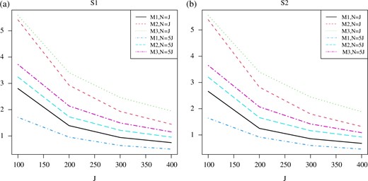
The loss |$\max_{3\leqslant K\leqslant 5} \{(NJ)^{-1/2} \|\hat{M}^{(K)}-M^* \|_\mathrm{F} \}$| for the recovery of the low-rank matrix |$M^*$|⁠, where each point is the mean loss calculated by averaging over 100 independent replications. Panels (a) and (b) show the results under the two different factor strength settings, S1 and S2, respectively.

Fig. 2.

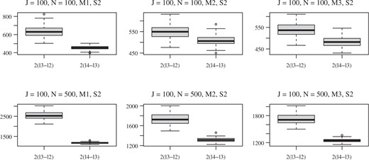
Box plots of |$2(\hat l_3 - \hat l_2)$| and |$2(\hat l_4 - \hat l_3)$| when |$J = 100$| and the factor strength setting is S2.

Table 1.

The number of times that the true number of factors is underselected or overselected among |$100$| independent replications under each of the |$48$| simulation settings

	|$N = J$|							|$N = 5J$|
	S1			S2				S1			S2
	M1	M2	M3	M1	M2	M3		M1	M2	M3	M1	M2	M3
Underselection
|$J = 100$|	0	0	0	0	0	0		0	0	0	10	98	97
|$J = 200$|	0	0	0	0	0	0		0	0	0	0	3	4
|$J = 300$|	0	0	0	0	0	0		0	0	0	0	0	0
|$J = 400$|	0	0	0	0	0	0		0	0	0	0	0	0
Overselection
|$J = 100$|	47	100	100	53	100	100		0	0	0	0	0	0
|$J = 200$|	0	94	90	0	100	95		0	0	0	0	0	0
|$J = 300$|	0	0	0	0	0	0		0	0	0	0	0	0
|$J = 400$|	0	0	0	0	0	0		0	0	0	0	0	0

From the results in Table 1, we see that for relatively small values of |$N$| and |$J$| the proposed information criterion tends to overpenalize when |$N = 5J$| and underpenalize when |$N=J$|⁠. We explain this phenomenon. Our choice of |$v(n,N,\,J,\,K)$| is derived from the error bound (5) in Theorem 1. Although this error bound is rate optimal as implied by Proposition 1, it does not take into account the relationship between |$N$| and |$J$|⁠. For example, consider two settings that both have no missing data and the same |$J$|⁠, but one with |$N = J$| and the other with |$N=5J$|⁠. By Theorem 1, the two settings have exactly the same upper bound |$\kappa(K_{\max}/J)^{1/2}$|⁠. However, as we can see from Fig. 1, the error tends to be larger under the setting when |$N=J$| than when |$N =5J$|⁠. Consequently, with the joint-likelihood-based information criterion derived from the same upper bound, it is more likely to overselect when |$N=J$| and to underselect when |$N=5J$|⁠. To improve the current information criterion a refined error bound is needed, according to which we can choose a |$v(n,N,\,J,\,K)$| that better adapts to the relationship between |$N$| and |$J$|⁠. This is a challenging problem and we leave it for future investigation.

4.2. Application to Eysenck’s personality questionnaire

We apply our proposed information criterion to a dataset based on the revised Eysenck personality questionnaire (Eysenck et al., 1985), a personality inventory that has been widely used in clinics and research. This questionnaire is designed to measure three personality traits: extraversion, neuroticism and psychoticism. We refer the reader to Eysenck et al. (1985) for the characteristics of these personality traits. The factor structure of this personality inventory remains of interest in psychology, due to its importance in the literature of human personality and wide use in several studies worldwide (Barrett et al., 1998; Chapman et al., 2013; Heym et al., 2013). In particular, it has been found that the dependence between items measuring the psychoticism trait tends to be lower than between items measuring the other two traits. Based on this observation, some researchers suggested that psychoticism may consist of multiple dimensions (Caruso et al., 2001). We use our proposed information criterion to investigate the factor structure of the inventory.

Specifically, we analyse all the items from the questionnaire, except for the lie scale items that are used to guard against various concerns about response style. There are 79 items in total, each with ‘Yes’ and ‘No’ response options. An example item is ‘Do you often need understanding friends to cheer you up?’. Among the 79 items, 32, 23 and 24 are designed to measure psychoticism, extraversion and neuroticism, respectively. For each participant, a total score can be computed based on each of the three item sets. This total score is often used to measure the corresponding personality trait. Here, we analyse a female UK normative sample dataset (Eysenck et al., 1985), for which the sample size is 824 and there are no missing values. The dataset was analysed in Chen et al. (2019) using the same model given in Example 1. Using a cross-validation approach, Chen et al. (2019) find three factors. We now explore the dimensionality of the data using our proposed information criterion. Specifically, we consider possible choices of |$K = 1, 2, 3, 4$|⁠, and |$5$|⁠. Following the previous discussion, the penalty term in our information criterion is set to |${K}({N \vee J})\log\{n /(N \vee J)\}$|⁠, where |$n = NJ$|⁠, |$N = 824$| and |$J = 79$|⁠.

The results are given in Tables 2 and 3. Specifically, the minimum jic value, indicated by the value in italics in Table 2, is achieved by the three-factor model suggesting a three-factor structure for the inventory. To obtain a relatively simple loading structure, we investigate the three-factor model using the oblimin method, one of the most popular oblique rotation methods ( Browne, 2001). Table 3 shows Kendall’s tau rank correlation between participants’ estimated factor scores under the oblimin rotation and the total scores for the three personality traits given by the design. The highest Kendall’s tau rank correlation in each row is in italics and is close to one, and the rest are close to zero which suggests that the extracted factors tend to correspond to the extraversion, psychoticism and neuroticism traits, respectively. Additional results can be found in the Supplementary Material, including the estimated parameters for the fitted models and a comparison with marginal-likelihood-based inference.

Table 2.

The rows show the values of |$-2 \hat l_K$|⁠, |$v(n,N,\,J,\,K)$| and jic, respectively, for models with different values of |$K$|

|$K$|	1	2	3	4	5
Deviance	63263	57683	53883	51225	48812
Penalty	3600	7201	10801	14402	18002
jic	66864	64884	64684	65627	66814

Table 3.

Kendall’s tau rank correlation between participants’ estimated factor scores under the oblimin rotation and the total scores for the three personality traits

	F1	F2	F3
P score	0.08	0.78	|$-$|0.05
E score	0.86	0.00	|$-$|0.12
N score	|$-$|0.08	0.08	0.88

5. Further discussion

As shown in § 3, there is a wide range of penalties for guaranteeing the selection consistency of jic. Among these choices, |$v(n,N,\,J,\,K) = {K}({N \vee J})\log\{n/(N\vee J)\}$| is close to the lower bound. This penalty is suggested when the signal strength of factors is unknown, to detect factors of a wide range of strengths. The performance and applicability of this information criterion are demonstrated by simulation studies and real data analysis. If one is only interested in detecting strong factors, then a larger penalty may be chosen based on prior information about the signal strength of the factors.

When our model (1) takes the form of a Gaussian density and there is no missing data, then our proposed information criterion and its theory are consistent with the results of Bai & Ng (2002) for high-dimensional linear factor models. In this sense, the current work substantially extends the work of Bai & Ng (2002) by considering nonlinear factor models and allowing a general setting for missing values. Although we focus on generalized latent factor models with an exponential-family link function, our proposed information criterion is applicable to other models, for example, a probit factor model for binary data that replaces the logistic link by a probit link in Example 1. The consistency results are likely to hold under similar conditions, for a wider range of models. This extension is left for future investigation.

Acknowledgement

We are grateful to the editor, the associate editor and three referees for their careful review and valuable comments. Li’s research was partially supported by the National Science Foundation (DMS-1712657).

Supplementary material

Supplementary Material includes technical proofs of the theoretical results, discussions on the computation, comparisons with related methods, and additional simulation and real data results.