Localized conformal prediction: a generalized inference framework for conformal prediction

Summary

We propose a new inference framework called localized conformal prediction. It generalizes the framework of conformal prediction by offering a single-test-sample adaptive construction that emphasizes a local region around this test sample, and can be combined with different conformal scores. The proposed framework enjoys an assumption-free finite sample marginal coverage guarantee, and it also offers additional local coverage guarantees under suitable assumptions. We demonstrate how to change from conformal prediction to localized conformal prediction using several conformal scores, and we illustrate a potential gain via numerical examples.

1. Introduction

Conformal prediction is an increasingly popular framework for measuring prediction uncertainty. Let |$Z_i:= (X_i, Y_i)$||$(i=1,\ldots,n)$| be independent and identically distributed regression data from some joint distribution |${\mathcal{P}}_{XY}$|⁠, where |$X_i\in \mathbb{R}^p$| is the feature and |$Y_i\in\mathbb{R}$| is the response. Given a new feature |$X_{n+1}$| with its response |$Y_{n+1}$| unobserved, the goal of conformal prediction is to construct a prediction interval |$C(X_{n+1})$| that covers |$Y_{n+1}$| with probability at least |$\alpha$|⁠:

$$ \begin{equation}\label{eq:goal} {\mathbb{P}}\{Y_{n+1}\in C(X_{n+1})\}\geqslant \alpha \end{equation}$$

(1)

for some desired coverage level |$\alpha\in (0,1)$|⁠, usually close to 1. Setting |$Z_{n+1}=(X_{n+1}, Y_{n+1})$| as the |$(n+1)$|th observation, conformal prediction achieves (1) under the assumption that |$Z_{n+1}$| is also independently generated from |${\mathcal{P}}_{XY}$|⁠, without additional distributional assumptions on |${\mathcal{P}}_{XY}$| itself (Vovk et al., 2005, 2009; Shafer & Vovk, 2008;Lei & Wasserman, 2014; Lei et al., 2018).

Let |${\mathcal{Z}} = \{Z_1,\ldots,Z_{n+1}\}$| be the unordered set of feature-response pairs, including |$Z_{n+1}=(X_{n+1},Y_{n+1})$|⁠. Conformal prediction relies on a conformal score function |$V(\cdot)$| for the observation |$z=(x,y)$|⁠, whose form may also depend on the unordered data |${\mathcal{Z}}$|⁠, i.e., |$V(z) = V(z;{\mathcal{Z}})$|⁠. We consider score functions |$V(\cdot)$| where large values of |$V(z)$| indicate that |$z$| is less likely to be a sample from |${\mathcal{P}}_{XY}$|⁠. For instance, we may choose |$V(z)=|\hat\mu(x) - y|$|⁠, where |$\hat\mu(\cdot)$| is a prediction function learned from the data |${\mathcal{Z}}$| or from a separate independent dataset.

It is guaranteed that the |$V_i := V(Z_i)$| are exchangeable when |$Z_1,\ldots,Z_{n+1}$| are independent and identically distributed. Letting |$Q(\alpha; V_{1:{n+1}})$| denote the level-|$\alpha$| quantile of the empirical distribution of |$V_1,\ldots,V_{n+1}$|⁠, then

$$ \begin{equation}\label{eq:eq1} {\mathbb{P}}\{V_{n+1} \leqslant Q(\alpha; V_{1:n+1})\} \geqslant \alpha. \end{equation}$$

(2)

Conformal prediction constructs the level-|$\alpha$| prediction interval for |$Y_{n+1}$| by inverting the above relationship:

$$ \begin{equation}\label{eq:eq2} C(X_{n+1}) = [y\colon V(X_{n+1},y)\leqslant Q\{\alpha; V_{1:n}\cup V(X_{n+1},y)\}]. \end{equation}$$

(3)

If the form of |$V(z)=V(z;{\mathcal{Z}})$| also depends on |${\mathcal{Z}}$| then in (3) each score |$V_i=V(Z_i;{\mathcal{Z}})$| also depends on |$y$| and is understood to be evaluated at |$Z_{n+1}=(X_{n+1},y)$|⁠. By the guarantee (2), |$C(X_{n+1})$| constructed in this way satisfies (1) for any distribution |${\mathcal{P}}_{XY}$|⁠.

It is common in data applications for the conditional distribution of |$Y$| given |$X=x$| to be heterogeneous across different values of |$x \in \mathbb{R}^p$|⁠. We want the constructed prediction interval to adapt to this heterogeneity in such settings. However, by definition, the interval |$C(X_{n+1})$| from conformal prediction is based on the global exchangeability of the conformal scores |$V_1,\ldots,V_{n+1}$|⁠, and depends equally on scores where |$X_i$| is far from |$X_{n+1}$| as on scores where |$X_i$| is close to |$X_{n+1}$|⁠. To adapt to the heterogeneity of |$Y$| given |$X=x$|⁠, one active area of research has been to design the score function |$V(\cdot)$| to directly capture this heterogeneity, in a way so that the quantiles of |$V(\cdot)$| are more homogeneous across different |$x \in \mathbb{R}^p$| (Lei & Wasserman, 2014; Lei et al., 2018; Izbicki et al., 2019; Romano et al., 2019; Chernozhukov et al., 2021; Gupta et al., 2021). For example, Romano et al. (2019) considered the quantile regression score |$V(z) =\max\{\hat q_{\rm lo}(x)-y,y-\hat q_{\rm hi}(x)\}$|⁠, where |$\hat q_{\rm lo}(x)$| and |$\hat q_{\rm hi}(x)$| are estimated quantiles for the conditional distribution of |$Y$| given |$X=x$|⁠. However, this approach may yield deteriorated performance when these quantile functions are difficult to estimate for some regions.

In this paper, we take a different approach, and generalize the inference framework itself by weighting the conformal scores |$V_1,\ldots,V_n$| differently based on the observed feature value |$X_{n+1}$|⁠. Our method places more weight on scores |$V_i$| for which |$X_i$| belongs to a local region around |$X_{n+1}$|⁠. Performing conformal inference while emphasizing the unique role of |$X_{n+1}$| is an interesting and open problem, and we provide the first such generalization with theoretical guarantees. We call this generalized framework localized conformal prediction, which can be flexibly combined with recently developed conformal score functions.

The main idea of localized conformal prediction is to introduce a localizer around |$X_{n+1}$|⁠, and up-weight samples close to |$X_{n+1}$| according to this localizer. For example, we may take the localizer |$H(X_{n+1},X_i) = \exp(-5|X_i - X_{n+1}|)$|⁠, consider the weighted empirical distribution where |$V_i$| has weight proportional to |$H(X_{n+1},X_i)$|⁠, and include the value |$y$| in |$C(X_{n+1})$| if and only if |$V(X_{n+1}, y)$| is smaller than the |$\tilde\alpha$| quantile of this weighted distribution. As this weighted distribution is no longer exchangeable, we need to choose |$\tilde\alpha$| strategically to guarantee finite-sample coverage as described in (1).

We demonstrate the difference between localized conformal prediction and conformal prediction with a simple example: features |$X\sim \operatorname{Un}(-5,5)$| follow a uniform distribution on |$[-5,5]$|⁠, and the response |$Y$| given |$X$| follows a mean-zero normal distribution with heterogeneous variance across |$X$|⁠:

$$\begin{equation} Y\mid X \sim \begin{cases} \cos\bigg(\dfrac{\pi}{10}X_i\bigg)\times N(0,1) & \mbox{if } |X|\leqslant 4.5,\\2\times N(0,1) & \mbox{if } |X|> 4.5. \end{cases} \end{equation}$$

We fix the desired coverage level |$\alpha = 0.95$|⁠, take |$n=1000$| samples, and perform both conformal prediction and localized conformal prediction with the localizer |$H(X_{n+1},X_i)=\exp(-5|X_i-X_{n+1}|)$| and two score functions: (i) the regression score |$V(z) = |\mu(x)-y|=|y|$|⁠, where here |$\mu(x)=0$| (Lei et al., 2018), and (ii) the quantile regression score |$V(z) =\max\{\hat q_{\rm lo}(x)-y,y-\hat q_{\rm hi}(x)\}$| (Romano et al., 2019), where |$\hat q_{\rm lo}$| and |$\hat q_{\rm hi}$| are |$0.025$| and |$0.975$| quantile curves estimated from 2000 independent samples using a neural network model, as described in § 4. We refer to the two corresponding conformal prediction procedures as CR and CQR, and the two localized conformal prediction procedures as LCR and LCQR.

Figures 1(a) and 1(b) show the conformal confidence bands for |$V_{n+1}$| using CR/LCR and using CQR/LCQR, respectively. Figures 1(c) shows the inverted prediction interval for |$Y_{n+1}$| using the four procedures. The green curves in (c) represent the true level-|$\alpha$| confidence bands for |$Y$| given |$X$|⁠. This example demonstrates that, by definition, the CR and CQR intervals are homogeneous for |$V$|⁠. In this example, the CR intervals are furthermore homogeneous for |$Y$|⁠. CQR provides a heterogeneous prediction interval for |$Y$| by inverting the interval for |$V$|⁠. However, the true quantile functions are hard to estimate at the two ends, and thus some heterogeneity of |$V_{n+1}$| still remains for the quantile regression score. In comparison, localized conformal prediction introduces more flexibility by directly constructing intervals that are heterogeneous for |$V$|⁠. It yields an improvement even when applied to the quantile regression score, where it better captures the remaining heterogeneity. We summarize our contributions as follows.

Fig. 1.

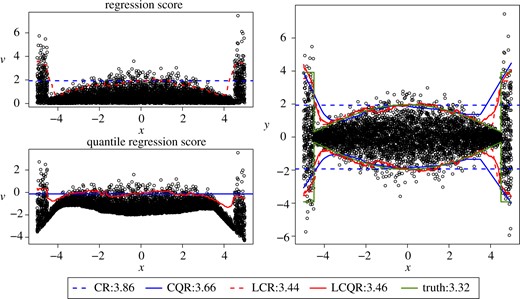
Comparison of conformal bands (CR, CQR) and localized conformal bands (LCR, LCQR) using regression and quantile regression scores. The left panels show the prediction bands for the conformal score |$V_{n+1}$|⁠, and the right panel shows the prediction bands response value |$Y_{n+1}$|⁠. True prediction bands for the distribution of Y given X are also shown on the right (truth), and dots show the realized test observation values in all plots. Values in the legends indicate the average prediction interval length associated with different approaches, which is shorter for the localized procedures.

• (i)

  We generalize the probabilistic framework of conformal prediction to localized conformal prediction, where we assign a unique role to the test point. The generalized framework still enjoys a distribution-free and finite-sample marginal coverage guarantee. Localized conformal prediction includes conformal prediction as a special case where the localizer takes a constant value.

• (ii)

  We develop an efficient implementation for sample-splitting localized conformal prediction. We also demonstrate how to combine it with some recently developed conformal scores with numerical examples.

• (iii)

  We investigate the local behaviour of sample-splitting localized conformal prediction and show that it enjoys additional local coverage guarantees under proper assumptions.

We defer all proofs to the Supplementary Material.

2. Localized conformal prediction

2.1. Notation

We use |${\mathbb{P}}\{\cdot\}$| to denote the probability of a given event. For any distribution |$\mathcal{F}$| on |$\mathbb{R}$|⁠, we define its level-|$\alpha$| quantile as

$$\begin{equation} Q(\alpha;\mathcal{F}) = \inf\{t\colon {\mathbb{P}}_{T\sim {\mathcal{F}}}\{T \leqslant t\} \geqslant \alpha\}. \end{equation}$$

Let |${\mathcal{X}}=\{X_1,\ldots, X_{n+1}\}$| be the unordered set of feature values from all |$n+1$| samples. Let |$H(x, x')\colon\mathbb{R}^p \times \mathbb{R}^p\mapsto [0,1]$| be a bivariate localizer function |$H(x, x')\colon\mathbb{R}^p \times \mathbb{R}^p\mapsto [0,1]$|⁠, whose function form may depend on the data through only |${\mathcal{X}}$|⁠. We require |$H(x, x) = 1$| for all |$x$| and use |$H(x, x')$| to capture the dissimilarity between two given feature values. In § 1, we considered |$H(x, x') = \exp(-5|x-x'|)$| as an example where |$H(X_{n+1},X_i)$| is the localizer evaluated at |$X_{n+1}$| and |$X_i$|⁠. The localizer function |$H(x,x')$| is used to construct different weighted distributions for performing localized conformal prediction. Define |$H_i(\cdot):= H(X_i, \cdot)$| as the localizer centred at |$X_i$|⁠, and |$H_{i,j} := H_i(X_j) = H(X_i, X_j)$| as a measure of dissimilarity between samples |$X_i$| and |$X_j$|⁠. Let |$\delta_v$| be a point mass at |$v\in \mathbb{R}$|⁠. Define weighted distributions

$$ \begin{align*} &\hat {\mathcal{F}}_i := \bigg(\sum^{n+1}_{j=1} p^H_{i,j}\delta_{V_j}\bigg)\quad (i = 1,\ldots, n+1), \end{align*}$$

where the empirical weights |$\smash{p^{H}_{i,j} := H_{ij}/(\sum^{n+1}_{k=1} H_{ik})}$| for |$j = 1,\ldots, n+1$| are constructed using the localizer centred at |$X_i$|⁠. We also define

$$ \begin{align*} &\hat {\mathcal{F}} := \bigg(\sum^{n}_{j=1} p^H_{n+1,j}\delta_{V_j}+p^H_{n+1,n+1}\delta_\infty\bigg) \end{align*}$$

as the distribution when replacing |$V_{n+1}$| by |$\infty$| in |$\smash{\hat{\mathcal{F}}_{n+1}}$|⁠. Both |$V_{n+1}$| and |$V_i$||$(i=1,\ldots, n)$| may depend on |$Y_{n+1}$| when |$V(\cdot)$| depends on the set |${\mathcal{Z}}$|⁠. Hence, there could be a dependence on |$Y_{n+1}$| from |$\smash{\hat{\mathcal{F}}}$| and |$\smash{\hat{\mathcal{F}}_i}$||$(i=1,\ldots, n+1)$|⁠. We have masked such a dependence for convenience.

Throughout this paper, we call |$\{Z_1,\ldots, Z_n\}$| the calibration set and assume that |$\smash{Z_i\overset{\text{i.i.d.}}{\sim} {\mathcal{P}}_{XY}}$| for |$i=1,\ldots, n+1,$| and |$\alpha\in (0,1)$| is a constant and user-specified targeted coverage.

2.2. Marginal coverage guarantee

We now establish the probabilistic guarantees of localized conformal prediction regarding its marginal coverage. Instead of using the level-|$\alpha$| quantile of the empirical distribution as in conformal prediction, localized conformal prediction considers a level-|$\tilde\alpha$| quantile of a weighted empirical distribution, with weight proportional to |$H_{n+1,i}$|⁠. Recall that |$H_{n+1,i}$| measures the distance between a training sample |$X_i$| and the test sample |$X_{n+1}$|⁠. This weighted distribution allows more emphasis on training samples closer to |$X_{n+1}$|⁠.

Theorem 1 below states how we can choose |$\tilde\alpha$| to achieve finite sample coverage. In Theorem 2 below we show that a randomized decision rule can lead to a prediction interval with exact coverage. Let |$\smash{\Gamma = \{ \sum_{k\in I_i}p^{H}_{ik}\colon i=1,\ldots,n+1, I_i \subseteq \{1,\ldots, n+1\}\}}$| represent all possible empirical cumulative distribution function values from weighted distributions |$\smash{\hat{\mathcal{F}}_i}$| for |$i=1,\ldots, n+1$|⁠, under all possible orderings of |$V_1,\ldots, V_{n+1}$|⁠.

 

Theorem 1.

Let |$\tilde\alpha$| be the smallest value in |$\Gamma$| such that

$$ \begin{equation}\label{eq:goal1general} (n+1)^{-1}\sum^{n+1}_{i=1}{\rm 1}\kern-0.24em{\rm I}_{V_i \leqslant Q(\tilde\alpha; \hat{\mathcal{F}}_i)} \geqslant \alpha. \end{equation}$$

(4)

Then |$\smash{{\mathbb{P}}\{V_{n+1} \leqslant Q(\tilde\alpha;\hat {\mathcal{F}}_{n+1} ) \}\geqslant \alpha}$|⁠. Equivalently, |$\smash{{\mathbb{P}}\{V_{n+1} \leqslant Q(\tilde\alpha;\hat {\mathcal{F}}) \}\geqslant \alpha}$|⁠.

 

Remark 1.

If |$H_{i,j} = 1$||$(i, j = 1,\ldots, n+1)$| then we have |$\smash{\hat {\mathcal{F}}=(n+1)^{-1}( \sum_{i=1}^n\delta_{V_i}+\delta_{\infty})}$| and |$\smash{\hat{\mathcal{F}}_i =(n+1)^{-1}( \sum_{i=1}^{n+1}\delta_{V_i})}$||$(i=1,\ldots, n+1)$|⁠. Then (4) holds if and only if |$\tilde\alpha\geqslant \alpha$| by definition. Also, |$\Gamma = \{k/(n+1)\colon k=1,\ldots, n+1\}$|⁠. Thus, we recover usual conformal prediction (Vovk et al., 2005), and

$$\begin{equation} {\mathbb{P}}\bigg\{V_{n+1} \leqslant Q\bigg(\frac{k}{n+1}; (n+1)^{-1}\sum_{i=1}^{n+1}\delta_{V_i}\bigg) \bigg\}\geqslant \alpha \quad\text{for }k \geqslant \lceil (n+1)\alpha\rceil. \end{equation}$$

Here, we provide some intuition for why such |$\tilde\alpha$| can guarantee level-|$\alpha$| coverage. Conformal prediction relies on the exchangeability of data. Conditional on the set |${\mathcal{Z}}$|⁠, the set of observed values |${\mathcal V}=\{v_1, \ldots, v_{n+1}\}$| for |$V_{1:(n+1)}$| is fixed and |$V_{n+1}$| has equal probability of taking each value in |${\mathcal V}$|⁠. Hence, |$\smash{Q\{\alpha, (n+1)^{-1}\sum_{i=1}^{n+1}\delta_{v_{i}}\}}$| leads to a coverage guarantee conditional on the observed values, and a marginal coverage guarantee after marginalizing over all value sets. When the prediction interval is constructed as |$Q(\tilde\alpha, \hat{\mathcal{F}}_{n+1})$|⁠, since |$\hat{\mathcal{F}}_{n+1}$| changes as we permute the value assignments, we need to account for this change when calculating the conditional coverage. The left-hand side of (4) turns out to be this coverage conditional on |$\{v_1, \ldots, v_{n+1}\}$| for any given |$\tilde\alpha$|⁠. As in conformal prediction, we can invert relationship (4) to construct a prediction interval for |$Y_{n+1}$|⁠.

 

Corollary 1.

In the setting of Theorem 1, define |$\tilde\alpha(y)\in \Gamma$| as the smallest value in |$\Gamma$| such that (4) holds at |$Z_{n+1}=(X_{n+1},y)$|⁠. Let |$C(X_{n+1}) := \{y\colon V_{n+1} \leqslant Q(\tilde\alpha(y);\hat {\mathcal{F}})\}$|⁠. Then, we have |${\mathbb{P}}\{Y_{n+1}\in C(X_{n+1})\}\geqslant \alpha$|⁠.

What will happen if we simply let |$\tilde\alpha = \alpha$| without tuning it based on (4)? The answer depends on the localizer |$H$|⁠. Setting |$\tilde\alpha=\alpha$| can lead to overcoverage in the simple example described by Proposition 1 below, where we tend to assign too little weight to the calibration samples. A more interesting example is given in Proposition 2 below, showing that we may end up achieving arbitrarily bad undercoverage by naively setting |$\tilde\alpha=\alpha$|⁠.

 

Proposition 1.

Consider the localizer |$H(x_1, x_2) =\exp\{-|x_1-x_2|/h\}$| with some small |$h>0$|⁠, such that |${\mathbb{P}}\{\sum^{n+1}_{i=1} H(X_{n+1}, X_i) < 1/(1-\alpha)\}\geqslant \varepsilon\in (\alpha,1)$|⁠. Then

$$ {\mathbb{P}}\{Q(\alpha;\hat{\mathcal{F}})=\infty\}\geqslant \varepsilon, \qquad {\mathbb{P}}\{V_{n+1}\in C(X_{n+1})\}\geqslant \varepsilon.$$

 

Proposition 2.

Let |$\{e_j\colon j = 1,\ldots, p\}$| be the standard basis in |$\mathbb{R}^p$|⁠. Set |$q_1 =(1-\alpha)/\{2p(1-\alpha)+\alpha\}$| and |$q_0 = \alpha/\{2p(1-\alpha)+\alpha\}$|⁠. Suppose that the feature |$X\in \mathbb{R}^p$| and response |$Y$| are distributed as

$$ \begin{align*} Y\mid X \sim \begin{cases} \operatorname{Un}(-1, 1)& \textit{when } X\,\,{={\hspace{-8pt}}|}\,\,\, 0,\\0& \textit{otherwise}, \end{cases} \quad X = \begin{cases} e_j & \textit{with probability } q_1 \textit{ for all } j =1,\ldots, p, \\ -e_j & \textit{with probability } q_1 \textit{ for all } j =1,\ldots, p,\\0 & \textit{with probability } q_0. \end{cases} \end{align*}$$

Let |$V(Z_i)=|Y_i|$| be the regression score. Then, for any constant |$p \geqslant 1$|⁠, we have |$\lim_{n\rightarrow\infty}{\mathbb{P}}\{V_{n+1}\leqslant Q(\alpha; \hat{\mathcal{F}})\}=q_0<\alpha$|⁠.

Proposition 2 shows that we no longer enjoy the distribution-free marginal coverage guarantee fixing |$\tilde\alpha=\alpha$|⁠, and the undercoverage can be arbitrarily poor for large |$p$|⁠. Hence, strategically choosing |$\tilde\alpha$| is crucial for a distribution-free marginal coverage guarantee, which is usually the motivation for using conformal prediction instead of other model-based prediction intervals.

As in the case of conformal prediction, we may not have exact level-|$\alpha$| coverage due to rounding issues. However, we can have exact |$\alpha$| coverage if we allow for some additional randomness, as stated in Theorem 2.

 

Theorem 2.

Consider the setting of Theorem 1. Let |$\tilde\alpha_1/\tilde\alpha_2$| be the smallest/ largest value in |$\Gamma\cup\{0\}$| such that

$$\begin{equation} \alpha_1:= (n+1)^{-1}\sum^{n+1}_{i=1}{\rm 1}\kern-0.24em{\rm I}_{V_i \leqslant Q(\tilde\alpha_1;\hat{\mathcal{F}}_i)} \geqslant \alpha, \qquad \alpha_2:= (n+1)^{-1}\sum^{n+1}_{i=1}{\rm 1}\kern-0.24em{\rm I}_{V_i \leqslant Q(\tilde\alpha_2;\hat{\mathcal{F}}_i)} < \alpha. \end{equation}$$

Set

$$\begin{equation} \tilde\alpha = \begin{cases} \tilde \alpha_1 & \textit{with probability }(\alpha - \alpha_2)/(\alpha_1-\alpha_2),\\\tilde\alpha_2 & \textit{with probability }(\alpha_1 - \alpha)/(\alpha_1-\alpha_2). \end{cases} \end{equation}$$

Then |${\mathbb{P}}\{V_{n+1} \leqslant Q(\tilde\alpha;\hat {\mathcal{F}} ) \}= \alpha$|⁠.

In this section, we presented localized conformal prediction with a potentially data dependent |$V(\cdot) = V(\cdot;{\mathcal{Z}})$|⁠, and showed that conformal prediction is its special case at |$H_{ij}=1$|⁠. The discussion of this general construction is for theoretical completeness, as the general recipe described in Theorem 1 or Corollary 1 is too computationally expensive: for every |$Y_{n+1}=y$|⁠, we need to retrain our prediction model to get |$V(\cdot;{\mathcal{Z}})$|⁠. This problem also exists for conformal prediction with data-dependent scores, and sample splitting is often used to reduce the computation cost (Papadopoulos et al., 2002; Lei et al., 2015).

For the remainder of this paper, we shift our focus to localized conformal prediction with sample splitting, where we divide the observed data into a training set and calibration set. The score function |$V(\cdot)$| is estimated with the training set and considered fixed afterward, and the prediction interval is constructed using the fixed score function and the calibration set.

3. Localized conformal prediction with sample splitting

3.1. Marginal coverage guarantee

We divide the observed data into the training set |$\mathcal{D}_0$| of size |$n_0$| and calibration set |$\mathcal{D}$| of size |$n$|⁠. We first construct the score function |$V(\cdot)$| based on |$\mathcal{D}_0$|⁠. For example, we may let |$V(Z) = |Y - \hat \mu(X)|$|⁠, where |$\hat \mu(\cdot)$| is a prediction function for |$Y$|⁠, learned using |$\mathcal{D}_0$|⁠. Since |$V(Z)$| does not depend on the calibration set and the test sample, we call it a fixed score function. We let |$\{Z_1, \ldots, Z_n\}$| denote samples of the calibration set, and |$Z_{n+1}$| the test sample. In this setting, because |$V(\cdot)$| is fixed, the empirical distributions |$\hat{\mathcal{F}}_i$| for |$i=1,\ldots, n+1$| depend on the value |$y$| of a test sample |$(X_{n+1},y)$| only via |$v=V(X_{n+1},y)$|⁠. Thus, |$\tilde\alpha(y)$| as defined in Corollary 1 depends on |$y$| only via |$v$|⁠. With a slight abuse of notation, we henceforth write |$\tilde\alpha(v)$| in place of |$\tilde{\alpha}(y)$|⁠, where |$v=V(X_{n+1},y)$|⁠. To make explicit the dependence of the empirical distribution |$\hat{\mathcal{F}}_i$| on |$v$|⁠, we introduce

$$ \begin{equation}\label{eq:hatFv} \hat{\mathcal{F}}_i(v) := \hat{\mathcal{F}}_i \quad\text{when}\quad V_{n+1} = v. \end{equation}$$

(5)

We express Theorem 1 and Corollary 1 for fixed |$V(\cdot)$| using Lemma 1 below, where we can also easily check that the resulting prediction interval for |$V_{n+1}$| is an interval.

 

Lemma 1.

Let |$V(\cdot)$| be a fixed score function. At |$V_{n+1} = v$|⁠, define |$\tilde\alpha(v)$| to be the smallest value of |$\tilde\alpha\in\Gamma$| such that

$$ \begin{equation*} (n+1)^{-1}\sum^{n+1}_{i=1}{\rm 1}\kern-0.24em{\rm I}_{V_i \leqslant Q\{\tilde\alpha; \hat{\mathcal{F}}_i(v)\}} \geqslant \alpha. \end{equation*}$$

Set |$C_V(X_{n+1}) = [v\colon v \leqslant Q\{\tilde\alpha(v);\hat {\mathcal{F}}\}]$|⁠, |$C(X_{n+1}) = \{y\colon V(X_{n+1},y)\in C_V(X_{n+1})\}$|⁠. Then |$C_V(X_{n+1})$| is an interval, and

$$\begin{equation} {\mathbb{P}}\{V_{n+1} \in C_V(X_{n+1}) \}\geqslant \alpha,\qquad {\mathbb{P}}\{Y_{n+1} \in C(X_{n+1}) \}\geqslant \alpha. \end{equation}$$

Lemma 1 is intuitively simple. However, even though the score function |$V(\cdot)$| is prespecified, it is still unrealistic to compute |$\tilde{\alpha}(v_{n+1})$| for every possible value |$v_{n+1} = V(X_{n+1}, y)$|⁠. In § 3.2 we provide an efficient implementation to tackle this problem.

3.2. An efficient implementation of localized conformal prediction

We provide an |$\mathcal{O}(n\log n)$| implementation of localized conformal prediction, given precalculated localizer function values for each pair of calibration samples and the associated unnormalized cumulative probabilities.

Without loss of generality, we assume that the calibration samples are ordered such that |$V_1\leqslant V_2\leqslant \cdots \leqslant V_n$|⁠. Let |$\overline{V}_i$| be the augmented observation with |$\overline{V}_i = V_i$||$(i = 1,\ldots, n)$|⁠, |$\overline{V}_{n+1} = \infty$| and |$\overline{V}_0 = -\infty$|⁠. For all |$i=1,\ldots, n+1$|⁠, we introduce the following definitions.

• (i)

  Let |$\ell(i)= \max\{i' \in \{1,\ldots,n\}\colon V_{i'}<\overline{V}_i\}$| be the largest index of |$V_{i'}$| smaller than |$\overline{V}_i$|⁠. When all |$V_i$| are distinct, |$\ell(i)=i-1$|⁠. We set the maximum of an empty set as 0, so in particular, |$\ell(1) = 0$| always.

• (ii)

  Let |$\theta_{i} := \sum_{j=1}^{\ell(i)}p^{H}_{i, j}$| be the cumulative probability at |$\overline{V}_{l(i)}$| in the distribution |$\hat{\mathcal{F}}_i(\infty)$|⁠.

• (iii)

  Let |$\tilde \theta_{i} := \sum_{j=1}^{\ell(i)}p_{n+1, j}^{H}$| be the cumulative probability at |$\overline{V}_{l(i)}$| in the distribution |$\hat{\mathcal{F}}$|⁠.

• (iv)

  Let |$\theta_i=\tilde\theta_{i} = 0$| if |$\ell(i) = 0$|⁠. In particular, |$\theta_{1} =\tilde\theta_1 = 0$| always.

Lemma 2 below is the foundation of our implementation. The first part of Lemma 2 describes a formulation to construct the closure of |$C_V(X_{n+1})$| from Lemma 1 that does not explicitly require calculation of |$\tilde{\alpha}(v_{n+1})$| for different values of |$v_{n+1}=V(X_{n+1},y)$|⁠. This formulation depends on a quantity |$S(k)$| defined in (6) below. The second part of Lemma 2 gives another equivalent characterization of |$S(k)$| that enables its calculation for all |$k=1,\ldots, n+1$| in |$\mathcal{O}(n\log n)$| time.

 

Lemma 2.

(Implementation of localized conformal prediction).

• (1)
  Let |$k^*$| be the largest index |$k \in \{1,\ldots,n+1\}$| such that

  $$ \begin{equation}\label{eq:goal1neg} S(k):= (n+1)^{-1}\sum_{i=1}^{n}{\rm 1}\kern-0.24em{\rm I}_{V_i \leqslant Q\{\tilde\theta_{k}; \hat{\mathcal{F}}_i(\overline{V}_{\ell(k)})\}} <\alpha. \end{equation}$$

  (6)

  Then |$\bar{C}_V(X_{n+1})=\{v\colon v\leqslant \overline{V}_{k^*}\}$| is the closure of |$C_V(X_{n+1})$| from Lemma 1.

• (2)
  Partition |$n$| calibration samples into three sets: |$A_1 := \{i\colon p_{i,n+1}^H + \theta_i < \tilde \theta_{{i}}\}$|⁠, |$A_2 := \{i\colon \theta_i \geqslant \tilde \theta_{{i}}\}$| and |$A_3 := \{i\colon p_{i,n+1}^H + \theta_i \geqslant \tilde \theta_{{i}},\,\theta_i < \tilde \theta_{{i}}\}$|⁠. For |$k = 1,\ldots, n+1$|⁠, we have

  $$ \begin{align}\label{eq:goal1equiv} S(k)=(n+1)^{-1}\bigg(\sum_{i\in A_1}{\rm 1}\kern-0.24em{\rm I}_{\theta_i+p_{i,n+1}^H < \tilde\theta_{k}}+\sum_{i\in A_2}{\rm 1}\kern-0.24em{\rm I}_{\theta_i < \tilde\theta_{k}}+\sum_{i\in A_3}{\rm 1}\kern-0.24em{\rm I}_{l(i)< {\ell(k)}}\bigg). \end{align}$$

  (7)

Here, we provide some intuition for why (6) and (7) are equivalent. Define the event |$J_{ik} = [V_i\leqslant Q\{\tilde\theta_k; \hat{\mathcal{F}}_i(\bar{V}_{\ell(k)})\}]$| in the indicator of (6). Observe that |$\tilde\theta_k$| and |$\overline{V}_{\ell(k)}$| are both nondecreasing in |$k$|⁠. Hence, the quantile |$Q\{\tilde\theta_k, \hat {\mathcal{F}}_i(\overline{V}_{\ell(k)})\}$| is also nondecreasing in |$k$|⁠, where we recall the definition of |$\hat {\mathcal{F}}_i(v)$| in (5). As a result, once |$J_{ik}$| holds for some |$k$|⁠, it also holds for all larger |$k$|⁠. For each |$i=1,\ldots,n$|⁠, we need only determine the smallest |$k$| for which |$J_{ik}$| first holds. There are two cases.

• (i)
  If |$J_{ik}$| first holds at a value |$k$| with |$V_i > \bar{V}_{\ell(k)}$|⁠, by the definition of |$\hat{\mathcal{F}}_i(\overline{V}_{\ell(k)})$|⁠, we need

  $$\begin{equation} \tilde\theta_k >\sum_{j\leqslant n\colon V_{j}< V_i}p^H_{i,j}+p^H_{i,n+1} = \theta_i+p^H_{i,n+1}. \end{equation}$$
• (ii)

  If |$J_{ik}$| first holds at a value |$k$| with |$V_i \leqslant \bar{V}_{\ell(k)}$| then we need |$\tilde\theta_k >\sum_{j\leqslant n\colon V_{j}< V_i}p^H_{i,j} = \theta_i$|⁠. To guarantee that |$V_i \leqslant \bar{V}_{\ell(k)}$|⁠, we also require that |$\ell(k) > \ell(i)$|⁠.

Let |$k_i$| be the smallest index |$k$| for which |$J_{ik}$| first holds. We can show that

• (a)

  |$A_1$| contains all |$i$| such that |$V_i > \bar{V}_{\ell(k_i)}$|⁠,

• (b)

  |$A_2$| contains all |$i$| such that |$V_i \leqslant \bar{V}_{\ell(k_i)}$| and |$\{\tilde\theta_{k_i} > \theta_i,\,\ell(k_i) > \ell(i)\} = \{\tilde\theta_{k_i} > \theta_i\}$|⁠,

• (c)

  |$A_3$| contains all |$i$| such that |$V_i \leqslant \bar{V}_{\ell(k_i)}$| and |$\{\tilde\theta_{k_i} > \theta_i,\,\ell(k_i) > \ell(i)\} = \{\ell(k_i) > \ell(i)\}$|⁠.

This will establish the equivalence between (6) and (7).

The desirable aspect of dividing calibration samples into |$A_1,A_2,A_3$| is that we can now order the calibration samples in each set based on the values of |$\theta_i+p^H_{i,n+1}$|⁠, |$\theta_i$| and |$l(i)$| for |$A_1,A_2$| and |$A_3$|⁠, respectively, and then compute all values |$S(k)$| from (7) using a single scan through the values |$k=1,\ldots,n+1$|⁠. Algorithm 1 below implements this idea. Line 1 calculates |$\tilde\theta_i$|⁠, |$\theta_i$| and |$\theta_i+p_{i,n+1}^H$| for each |$i=1,\ldots,n+1$|⁠; line 2 creates |$A_1,A_2,A_3$| according to Lemma 2. Line 3 orders |$i \in A_1$| by |$\theta_i+p_{i,n+1}^H$|⁠, |$i \in A_2$| by |$\theta_i$| and |$i \in A_3$| by |$l(i)$|⁠. As we increase |$k$|⁠, samples |$i$| in each set |$A_1,A_2,A_3$| will satisfy |$\smash{V_i \leqslant Q\{\tilde\theta_k; \hat{\mathcal{F}}_i(\overline{V}_{\ell(k)})\}}$| sequentially. Lines 5–6, 7–8 and 9–10 perform these sequential checks within each set |$A_1, A_2, A_3$|⁠. Finally, line 12 produces the largest |$k^*$| such that (6) holds for any given target level |$\alpha$|⁠.

Algorithm 1.

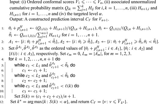
Localized conformal prediction.

3.3. Choice of H

The choice of |$H$| will influence the localization. Given |$d(x_1, x_2)$| as a measure of dissimilarity between two samples |$x_1$|⁠, |$x_2$|⁠, there are numerous ways of defining the functional form for the localizer. In our experiments, we consider the localizer |$H(x_1, x_2) = \exp\{-d(x_1, x_2)/h\}$|⁠.

A smaller |$h$| results in more localization. We prefer |$h$| resulting in a relatively narrow prediction interval for most samples. More specifically, we consider the constrained objective

$$ \begin{align*} J(h) =\ &\text{average of PI}^{\text{finite}}\text{ length}+\lambda\times \text{average of conditional PI}^{\text{finite}}\text{ length}'\text{s variability},\\& \text{such that the } \text{average percentage of infinite prediction intervals is at most }\varepsilon. \end{align*}$$

The parameter |$\lambda$| reflects our aversion to the variability of a constructed prediction interval’s length at each fixed point |$X_{n+1}=x$| in the feature space. We set |$\lambda=1$| by default.

These averages are unknown and need to be estimated from the data. Recall that the score function |$V(\cdot)$| is constructed using an independent training set |$\mathcal{D}_0$|⁠, whose model complexity is often tuned with cross-validation. We suggest using |$\mathcal{D}_0$| and its cross-validated scores to estimate the three terms in the above objective empirically. The mathematical definitions of |$J(h)$| and details of the empirical estimates are given in the Supplementary Material.

In low dimensions, we can have asymptotic conditional coverage as |$n\rightarrow \infty$| using typical distance dissimilarities, e.g., Euclidean distance, and by choosing |$h\rightarrow 0$| under suitable assumptions as shown in § 5. This is an ideal setting. In practice, a good user-specified dissimilarity function |$d(\cdot,\cdot)$| will lead to improved performance in terms of a constructed prediction interval length and adaptation to the underlying heterogeneity. Such a dissimilarity function should capture directions of feature space in which the prediction interval of |$V$| is more likely to vary. A comprehensive and in-depth discussion of |$d(\cdot,\cdot)$|⁠, especially in high dimensions, is beyond the scope of this paper. In our numerical experiments, we define |$d(\cdot,\cdot)$| as a weighted sum of three components:

• (i)

  |$d_1(x_1, x_2) = \|\hat\rho(x_1)-\hat\rho(x_2)\|_2$|⁠, where |$\hat\rho(X)$| is the estimated spread of |$V(X,Y)$| conditional on |$X$| (Lei et al., 2018);

• (ii)

  |$d_2(x_1, x_2) = \|P_{\parallel}(x_1 - x_2)\|_2$|⁠, where |$P_{\parallel}$| is the projection onto the space spanned by the top singular vectors of the Jacobian matrix of |$\hat\rho(X)$| for |$X\in \mathcal{D}_0$|⁠; and

• (iii)

  |$d_3(x_1, x_2) = \|P_{\perp}(x_1 - x_2)\|_2$|⁠, where |$P_{\perp}$| is the projection onto the space orthogonal to |$P_{\parallel}$|⁠.

We include the first component since |$\hat\rho(X)$| is trying to capture the heterogeneity of |$V(X,Y)$|⁠. We include the second and the third components to make the dissimilarity depend on other directions in the feature space because |$\hat\rho(X)$| may not fully capture the underlying heterogeneity. Intuitively, we can think of the projection |$P_{\parallel}$| as capturing the directions of feature space in which |$\rho(X)$| is more variable across the training set, and |$P_{\perp}$| as capturing the remaining less important directions. We provide more details on constructing |$d(\cdot,\cdot)$| in the Supplementary Material.

4. Empirical studies

This section compares localized conformal prediction and conformal prediction with different numerical examples. We consider the usual regression problem,

$$\begin{equation} Y= \mu(X)+\varepsilon, \qquad \varepsilon \perp\!\!\!\perp X, \end{equation}$$

and four types of conformal score construction.

• (i)

  Regression score: |$V^{R}(X, Y) = |Y - \hat \mu(X)|$|⁠, where |$\hat \mu(X)$| is an estimate of |$\mu(X)$| learned from the training set. We denote conformal prediction with regression score as CR and localized conformal prediction with regression score as LCR.

• (ii)

  Locally weighted regression score: |$V^{R\text{-local}}(X, Y) =V^{R}(X, Y)/\hat \rho(X)$|⁠, where |$\hat\rho(X)$| is the estimated spread of |$V^{R}(X,Y)$| (Lei et al., 2018). When combined with conformal prediction and localized conformal prediction, we denote the two resulting procedures as CLR and LCLR, respectively.

• (iii)

  Quantile regression score: |$V^{\rm QR}(X, Y) = \max\{\hat q_{\rm lo}(X_i) - Y, Y - \hat q_{\rm hi}(X)\}$|⁠, where |$\hat q_{\rm lo}(\cdot)$| and |$\hat q_{\rm hi}(\cdot)$| are the estimated lower and upper |$(\alpha/2)$| quantiles from the training set (Romano et al., 2019). When combined with conformal prediction and localized conformal prediction, we denote the two resulting procedures as CQR and LCQR, respectively.

• (iv)

  Locally weighted quantile regression score: |$V^{\text{QR-local}} =V^{\rm QR}(X, Y)/\hat \rho(X)$|⁠, which combines quantile regression with the locally weighted step. When combined with conformal prediction and localized conformal prediction, we denote the two resulting procedures as CLQR and LCLQR, respectively.

In Example 1 below we visually demonstrate conformal prediction and localized conformal prediction to highlight the procedural differences, and compare results from localized conformal prediction with different values for |$h$|⁠. In Example 2, we use synthetic data and compare the performance of the eight procedures. Example 3 compares the results using four publicly available datasets from UCI. We learn the conformal scores using a neural network with three fully connected layers and 32 hidden nodes in all empirical examples.

 

Example 1

(Conformal prediction and localized conformal prediction). Let |$Y = \varepsilon$|⁠, |$X\sim N(0, 1)$| and |$\varepsilon\sim \rho(X)$|⁠, with four different cases for |$\rho(X)$|⁠: (A) |$\rho(X) = \sin(X)$|⁠; (B) |$\rho(X) = \cos(X)$|⁠; (C) |$\rho(X) = \surd{|X|}$|⁠; (D) |$\rho(X) = 1$|⁠. We compare conformal prediction, the autotuned localized conformal prediction described in § 3.3 and localized conformal prediction using fixed |$h$| values. The prefixed grids for |$h$| can be different for different settings because they are chosen by looking at the dissimilarity measures on the training set. The sizes for the training and calibration sets are both 1000. Table 1 compares conformal regression with autotuned localized conformal prediction, and shows the achieved coverage, percentage of samples with infinite prediction interval and the average length of the finite prediction interval. Table 2 compares localized conformal prediction from using different |$h$|⁠. Figure 2 provides visual demonstrations for conformal prediction and localized conformal prediction using |$h_1$|⁠, the smallest |$h$| with less than 5|$\%$| of infinite prediction interval for localized conformal prediction; |$h_2$|⁠, the largest |$h$| considered; and |$h_3$|⁠, the autotuned |$h$|⁠. The choice of |$h_1$| results in a highly localized conformal prediction with the prediction interval better capturing the underlying heterogeneity, but potentially less stable and containing the infinite prediction interval with higher probability, while the choice of |$h_2$| results in a prediction interval with almost no localization and almost identical to conformal prediction.

Fig. 2.

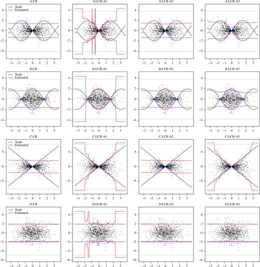
(Example 1.) Confidence bands constructed using conformal prediction (CR) and localized conformal prediction (LCR) with different tuning parameter values for |$h$| at the targeted level |$\alpha = 0.95$|⁠. In each subplot, we show the test data points with dots, and the true confidence bands and estimated confidence intervals across different |$X_{n+1}$| are represented by different colors as described in the legends. We sometimes encounter infinite prediction intervals using localized conformal prediction and represent these by widths larger than the grey horizontal lines.

Table 1.

(Example 1) Coverage and length comparisons for conformal prediction and localized conformal prediction (autotuned) across four simulation set-ups. We also underline the smallest ave.PI, which is the average prediction interval length using finite prediction intervals, and those within 0.05 from it in different settings

	Setting (A)		Setting (B)		Setting (C)		Setting (D)
	CR	LCR	CR	LCR	CR	LCR	CR	LCR
Coverage	0.95	0.94	0.95	0.95	0.95	0.95	0.94	0.94
Infinite PI|$\%$|	–	0.00	–	0.00	–	0.01	–	0.00
ave.PI	2.77	2.27	3.14	3.01	4.26	3.15	3.81	3.86

CR, conformal prediction; LCR, localized conformal prediction.

Table 2.

(Example 1) Comparisons of the coverage, percentage of infinite prediction interval, ave.PI and ave.PI0 for different tuning parameters |$h$|⁠, where ave.PI is the average length for finite prediction intervals at the given |$h$|⁠, and ave.PI0 is the average length for finite prediction intervals across all |$h$| considered. We underline all ave.PI0 for |$h$| no greater than the autotuned |$\hat h$| in each setting

Setting (A)
|$h$|	0.05	0.07	0.09	0.13	0.17	0.22	0.29	0.39	0.52	0.69	0.91	1.21	1.61	2.14	2.84	3.78	5.01	6.66	8.84	11.74
Coverage	0.95	0.95	0.95	0.95	0.95	0.95	0.95	0.95	0.95	0.95	0.94	0.95	0.95	0.95	0.95	0.95	0.95	0.95	0.95	0.95
Infinite PI|$\%$|	0.23	0.15	0.07	0.04	0.02	0.01	0.01	0.01	0.00	0.00	0.00	0.00	0.00	0.00	0.00	0.00	0.00	0.00	0.00	0.00
ave.PI	2.22	2.27	2.27	2.28	2.29	2.32	2.32	2.32	2.32	2.29	2.27	2.36	2.43	2.51	2.57	2.61	2.67	2.70	2.71	2.74
ave.PI0	2.22	2.21	2.20	2.18	2.19	2.23	2.24	2.26	2.25	2.22	2.22	2.32	2.40	2.49	2.55	2.61	2.66	2.69	2.70	2.73
Setting (B)
|$h$|	0.08	0.1	0.13	0.18	0.24	0.32	0.43	0.57	0.76	1.02	1.36	1.81	2.42	3.24	4.32	5.77	7.7	10.28	13.73	18.33
Coverage	0.94	0.95	0.95	0.94	0.94	0.95	0.94	0.94	0.95	0.95	0.95	0.95	0.95	0.95	0.95	0.95	0.95	0.95	0.95	0.95
Infinite PI|$\%$|	0.17	0.09	0.07	0.05	0.04	0.03	0.01	0.01	0.00	0.00	0.00	0.00	0.00	0.00	0.00	0.00	0.00	0.00	0.00	0.00
ave.PI	2.81	2.68	2.67	2.63	2.65	2.65	2.66	2.73	2.82	2.87	2.98	3.01	3.03	3.07	3.08	3.11	3.12	3.13	3.13	3.13
ave.PI0	2.81	2.81	2.84	2.81	2.83	2.83	2.84	2.89	2.96	2.98	3.06	3.07	3.07	3.10	3.11	3.13	3.13	3.14	3.13	3.14
Setting (C)
|$h$|	0.04	0.06	0.09	0.12	0.17	0.24	0.33	0.46	0.65	0.91	1.27	1.78	2.49	3.48	4.87	6.83	9.56	13.38	18.74	26.23
Coverage	0.94	0.94	0.94	0.94	0.95	0.95	0.95	0.95	0.95	0.95	0.95	0.95	0.95	0.95	0.95	0.95	0.95	0.95	0.95	0.95
Infinite PI|$\%$|	0.29	0.22	0.14	0.09	0.07	0.05	0.03	0.02	0.01	0.01	0.00	0.00	0.00	0.00	0.00	0.00	0.00	0.00	0.00	0.00
ave.PI	1.88	2.12	2.42	2.68	2.81	2.87	3.02	3.08	3.15	3.24	3.34	3.48	3.62	3.80	3.94	4.01	4.10	4.16	4.19	4.21
ave.PI0	1.88	1.88	1.87	1.91	1.91	1.93	1.99	2.06	2.20	2.44	2.65	2.97	3.25	3.57	3.80	3.90	4.03	4.12	4.16	4.19
Setting (D)
|$h$|	0.08	0.11	0.15	0.2	0.28	0.38	0.53	0.73	1.00	1.38	1.9	2.61	3.6	4.95	6.82	9.4	12.94	17.82	24.54	33.8
Coverage	0.94	0.95	0.94	0.94	0.95	0.94	0.94	0.94	0.94	0.94	0.94	0.94	0.94	0.94	0.94	0.94	0.94	0.94	0.94	0.94
Infinite PI|$\%$|	0.14	0.10	0.05	0.02	0.01	0.01	0.01	0.00	0.00	0.00	0.00	0.00	0.00	0.00	0.00	0.00	0.00	0.00	0.00	0.00
ave.PI	3.79	3.85	3.92	3.92	3.92	3.90	3.89	3.92	3.89	3.89	3.89	3.87	3.86	3.86	3.88	3.87	3.87	3.86	3.85	3.85
ave.PI0	3.79	3.80	3.80	3.78	3.82	3.82	3.82	3.86	3.84	3.85	3.86	3.85	3.84	3.86	3.87	3.87	3.86	3.86	3.85	3.84

We do not observe an increased average prediction interval length on samples well represented by the calibration set as we decrease |$h$| in a wide range. A smaller |$h$| makes the procedure more alert by producing infinite prediction intervals for under-represented new observations. Is this a bad thing? We believe that the answer to this question is subjective and depends on the specific task at hand.

 

Example 2

(Comparisons of different procedures; synthetic data). We now compare eight procedures by applying conformal prediction and autotuned localized conformal prediction to four different conformal scores regarding their coverage and prediction interval lengths at a targeted level |$\alpha = 0.95$|⁠. We consider the same simulation set-up as in Example 1 except with |$X\sim {\mbox{Un}}(-2,2)$|⁠. In this example, the test observations are reasonably well represented by the calibration samples, with high probability. We do not observe samples with infinite prediction intervals using autotuned localized conformal prediction. Tables 3 and 4 show the results of the average coverage and average length of the prediction interval in the four simulation settings.

Table 3.

(Example 2) Empirical coverage for different procedures across different simulation settings, with a targeted level at |$\alpha = 0.95$|

	CR	LCR	CLR	LCLR	CQR	LCQR	CLQR	LCLQR
Setting (A)	0.952	0.955	0.953	0.954	0.953	0.955	0.953	0.954
Setting (B)	0.951	0.953	0.950	0.954	0.953	0.953	0.953	0.954
Setting (C)	0.948	0.950	0.949	0.950	0.950	0.951	0.951	0.952
Setting (D)	0.948	0.948	0.948	0.949	0.948	0.948	0.947	0.948

CR, conformal prediction; LCR, localized conformal prediction; CLR, conformal prediction with locally weighted regression score; LCLR, localized conformal prediction with locally weighted regression score; CQR, conformal prediction with quantile regression score; LCQR, localized conformal prediction with quantile regression score; CLQR, conformal prediction with locally weighted quantile regression score; LCLQR, localized conformal prediction with locally weighted quantile regression score.

Table 4.

(Example 2) Average lengths of prediction intervals for different procedures across four different simulation settings. We underline the smallest average prediction interval length and those within 0.05 from it in each setting

	CR	LCR	CLR	LCLR	CQR	LCQR	CLQR	LCLQR
Setting (A)	3.27	2.84	3.05	2.81	2.87	2.87	2.88	2.87
Setting (B)	2.86	2.19	2.54	2.20	2.26	2.27	2.27	2.27
Setting (C)	4.95	3.91	4.42	3.90	3.94	3.95	4.03	4.02
Setting (D)	3.88	3.90	3.89	3.90	3.92	3.93	3.92	3.93

See Table 3 for abbreviations.

 

Example 3

(Performance comparison using four datasets). We investigate the performances of eight procedures using conformal prediction and autotuned localized conformal prediction on four UCI datasets (Dua & Graff, 2019): CASP (Yeh, 1998), Concrete (Yeh, 1998), Facebook variant 1, denoted as facebook1, and Facebook variant 2, denoted as facebook2 (Singh, 2015; Singh et al., 2015). The sizes of samples and features are |$(45\,730, 9)$|⁠, |$(1030, 8)$|⁠, |$(40\,949, 53)$|⁠, |$(81\,312, 53)$| for the four datasets, respectively.

We subsample 5000 training/calibration samples without replacement from CASP, facebook1 and facebook2, and 400 training/calibration samples from the Concrete dataset. We construct prediction intervals using the remaining samples for each dataset and repeat it 20 times. Tables 5–6 show the results of the average coverage and average length of the finite prediction interval for the four datasets. The percentage of infinite prediction intervals ranges from 0|$\%$| to 3|$\%$| for different localized conformal prediction procedures. The samples with infinite prediction interval using localized conformal prediction on the Facebook datasets tend to have wider prediction intervals; hence, we also show the average prediction interval length using only samples with finite prediction interval from all procedures for a fair comparison.

The conformal quantile regression procedure has been shown as a top performer in Romano et al. (2019) and Sesia & Candès (2020). Our numerical experiments also confirm that it has an overall better performance than the conformal prediction with locally weighted regression score. Not only is localized conformal prediction conceptually novel, but it also uses the estimated spread |$\hat \rho(X)$| in a more robust way. When combined with |$V^{R}$| and |$V^{R\text{-local}}$|⁠, the average prediction interval lengths are smaller for three out of the four real datasets compared with the conformal prediction with locally weighted regression score procedure. In particular, localized conformal regression and localized conformal prediction with the locally weighted regression score are even noticeably better than conformal quantile regression in the two Facebook examples.

Table 5.

(Example 3) Empirical coverage for different procedures, with |$\alpha = 0.95$|

	CR	LCR	CLR	LCLR	CQR	LCQR	CLQR	LCLQR
CASP	0.949	0.950	0.950	0.950	0.950	0.950	0.950	0.950
Concrete	0.947	0.949	0.943	0.947	0.951	0.953	0.952	0.954
facebook1	0.949	0.950	0.949	0.949	0.950	0.951	0.950	0.951
facebook2	0.951	0.951	0.951	0.951	0.953	0.952	0.953	0.952

See Table 3 for abbreviations.

Table 6.

(Example 3) The upper half shows the average length using samples with finite prediction intervals for the given procedure. The lower half shows the average prediction interval length on the common set of samples with finite prediction interval for all pro- cedures. We underline the smallest average prediction interval length and those within 0.05 from it in each setting

Procedure-specific samples
	CR	LCR	CLR	LCLR	CQR	LCQR	CQLR	LCQLR
CASP	3.03	2.82	2.88	2.81	2.65	2.64	2.65	2.64
Concrete	1.52	1.48	1.45	1.46	1.58	1.59	1.58	1.57
facebook1	1.12	0.67	|$>100$|	0.69	0.92	0.92	0.92	0.92
facebook2	1.05	0.65	|$>100$|	0.65	0.92	0.92	0.93	0.92
Common samples
	CR	LCR	CLR	LCLR	CQR	LCQR	CQLR	LCQLR
CASP	3.03	2.82	2.88	2.81	2.65	2.64	2.65	2.64
Concrete	1.52	1.47	1.43	1.45	1.56	1.56	1.56	1.55
facebook1	1.12	0.66	0.95	0.66	0.74	0.74	0.74	0.74
facebook2	1.05	0.62	0.87	0.63	0.74	0.74	0.74	0.74

See Table 3 for abbreviations.

5. Local behaviour of localized conformal prediction

In this section, we consider asymptotic and approximate conditional coverage properties for localized conformal prediction and a simplified version fixing |$\tilde\alpha=\alpha$|⁠. We have shown in Proposition 2 that this simplified localized conformal prediction does not yield a distribution-free coverage guarantee. Our results here indicate that it could lead to asymptotic or approximate conditional coverage, under certain assumptions.

For simplicity, we restrict attention to the localizer |$H(x_1, x_2) =\exp\{-d(x_1, x_2)/h_n\}$|⁠, where |$h_n$| is an |$n$|-dependent bandwidth parameter, and |$d(x_1, x_2)\geqslant 0$| is a measure of dissimilarity satisfying |$d(x_1, x_1) = 0$|⁠.

First, we consider the asymptotic conditional coverage. Nontrivial finite sample and distribution-free conditional coverage is impossible for continuous distributions (Vovk, 2013; Lei & Wasserman, 2014). Thus, it is common to consider asymptotic conditional coverage under proper assumptions on |$\mathcal{P}_{XY}$|⁠. Different conformal score constructions with such asymptotic conditional coverage are studied in the literature. For instance, Izbicki et al. (2019) considered using the estimated conditional density as the conformal score, and Romano et al. (2019) used the conformal score based on estimated quantile functions. Here, we consider the asymptotic behaviour of localized conformal prediction.

 

Assumption 1.

It holds that |$X$| has continuous distribution on |$[0,1]^p$|⁠, and |$V(Z)$| has continuous distribution conditional on |$X=x$|⁠. Furthermore, there exist constants |$L>0$| and |$\beta\geqslant 0$| such that the density of |$X$| satisfies |$p_X(x)\geqslant 1/ L$| for all |$x \in [0,1]^p$|⁠, and

• (i)
  for all |$x,x' \in [0,1]^p$|⁠, the conditional distribution of |$V$| given |$X$| satisfies

  $$\begin{equation} \max_{v\in \mathbb{R}}|P_{V\mid x}(v)-P_{V\mid x'}(v)|\leqslant L d(x, x'), \end{equation}$$

  where |$P_{V\mid x}(v)$| is the probability of |$V(Z)\leqslant v$| conditional on |$X= x$|⁠;
• (ii)

  |${\mathbb{P}}[X\in \{x\colon d( x_0, x) \leqslant \varepsilon\}] \geqslant \varepsilon^{\beta}/L$| for all |$\varepsilon \leqslant h_n$| and all |$x_0\in [0,1]^p$|⁠;

• (iii)

  |$h_n$| is chosen such that |$h_n\rightarrow 0$| and |$n h_n^\beta/ \ln n\rightarrow \infty$| as |$n\rightarrow \infty$|⁠.

Under this assumption, statement (8) of the following theorem guarantees that localized conformal prediction with |$\tilde\alpha(v)$| chosen as in Lemma 1 achieves asymptotic conditional coverage at the target level |$\alpha$|⁠. Furthermore, statements (9) and (10) below show that |$\tilde\alpha(v)$| converges to |$\alpha$| asymptotically, and asymptotic conditional coverage also holds for the simplified version.

 

Theorem 3.

Define |$\tilde\alpha(v)$| and |$C_V(X_{n+1})$| as in Lemma 1. Under Assumption 1, for any |$x_0 \in [0,1]^p$|⁠, we have

$$ \begin{align} &\lim_{n\rightarrow\infty}{\mathbb{P}}\{V_{n+1}\in C_V(X_{n+1})\mid X_{n+1}=x_0\} =\alpha,\label{eq:thmAsy1} \end{align}$$

(8)

$$ \begin{align} &\lim_{n\rightarrow\infty}{\mathbb{P}}\{V_{n+1}\leqslant Q(\alpha; \hat{\mathcal{F}})\mid X_{n+1}=x_0\}= \alpha,\label{eq:thmAsy2} \end{align}$$

(9)

$$ \begin{align} &\lim_{n\rightarrow\infty}{\mathbb{P}}\Big\{\max_{v}|\tilde\alpha(v)-\alpha |<\varepsilon\Bigm|X_{n+1}=x_0\Big\} =1 \quad\text{for all }\varepsilon > 0.\label{eq:thmAsy3} \end{align}$$

(10)

In Assumption 1, the measure |$d(x, x')$| can be defined to capture the directions where the conditional distribution of |$V$| given |$X$| is more likely to change as we vary |$X$|⁠. Assumption 1(i) allows more variability in some directions and less in others based on how the data are generated, and scales better with the dimension compared to a symmetric distance such as the Euclidean distance. Assumption 1(ii) assumes that |$d(x_0,x)$| has enough concentration around 0, and it holds for a typical dissimilarity measure in low dimensions. In high dimensions, this assumption holds if |$d(\cdot,\cdot)$| emphasizes a few directions instead of treating all directions equally. For example, if |$d(x_0,x) = |x_j - x_{0,j}|$| depends only on feature |$j$| then |${\mathbb{P}}\{X\colon d(x_0,X)\leqslant \varepsilon\}\geqslant\varepsilon/L$| for some large constant |$L$|⁠. Assumption 1(iii) requires |$h_n$| to decay to 0 at a sufficiently slow rate. This is so that, combined with Assumption 1(ii), we may ensure that |$\sum_{i=1}^{n} H(X_j, X_i) \to \infty$| for all |$j=1,\ldots,n+1$|⁠, with high probability. In particular, a setting such as described in Proposition 1 cannot occur.

Next, we consider the approximate conditional coverage. Vovk (2013) and Lei & Wasserman (2014) partitioned the feature space into |$K$| finite subsets and applied conformal inference to each of the subsets: this guarantees that |${\mathbb{P}}\{Y_{n+1}\in {\hat C}(X_{n+1})\mid X_{n+1}\in \mathcal{X}_k\} \geqslant \alpha$| for all |$k = 1,2,\ldots, K$| and some fixed partition |$\smash{\bigcup^K_{k=1} \mathcal{X}_k = \mathbb{R}^p}$|⁠. Barber et al. (2020b) considered a potentially stronger version where different regions |$\mathcal{X}_k$| may overlap. Barber et al. (2020a) introduced a different notion of approximate conditional coverage, where instead of finding |$C(x_0)$| that achieves conditional coverage of |$Y_{n+1}$| given |$X_{n+1}=x_0$|⁠, the authors considered |$C(x_0)$| that covers |$\tilde Y$| whose feature value |$\tilde X$| is distributed according to some locally weighted distribution around |$x_0$|⁠, as described in equations (18)–(19) of Barber et al. (2020a). When this weighted distribution becomes increasingly concentrated around |$x_0$|⁠, the distribution of |$\tilde Y$| intuitively approaches the conditional distribution of |$Y_{n+1}$|⁠, so this serves as an approximation to conditional coverage. Here, we show that, for a local weighting given by |$H(x_0,x)=\exp\{-d(x_0, x)/h_n\}$|⁠, an adjusted localized conformal prediction procedure with the aforementioned |$H(\cdot,\cdot)$| as its localizer, |$\tilde\alpha=\alpha$|⁠, and an additional slacking term, can achieve this guarantee for every fixed |$x_0$|⁠.

 

Theorem 4.

Define the weighted distribution |$d \tilde {\mathcal{P}}^{x_0}_X(x)/{\rm d} x \propto H(x_0, x)$||$d {\mathcal{P}}_X(x)/{\rm d} x$|⁠. Conditional on |$X_{n+1}=x_0$|⁠, let |$\tilde Z=(\tilde X, \tilde Y)\sim \tilde {\mathcal{P}}_{X}^{x_0}\times {\mathcal{P}}_{Y\mid X}$|⁠. Define

$$ \begin{align*} \varepsilon(X_{n+1})&=\max_{x\colon d(X_{n+1},x)<\infty}\max_y|V(X_{n+1},y)-V(x,y)|,\\\tilde C(X_{n+1}) &= \{y\colon V(X_{n+1},y)\leqslant Q(\alpha; \hat{\mathcal{F}})+\varepsilon(X_{n+1})\}, \end{align*}$$

where |$d(\cdot,\cdot)$| is the dissimilarity measure that defines |$H(\cdot,\cdot)$|⁠. Then

$$ \label{eq:approxmateLCP} {\mathbb{P}}\{V(\tilde Z)\leqslant Q(\alpha; \hat{\mathcal{F}})\mid X_{n+1} = x_0\}\geqslant \alpha, \qquad {\mathbb{P}}\{\tilde Y\in \tilde C(X_{n+1})\mid X_{n+1} = x_0\}\geqslant \alpha. $$

The interval |$\tilde{C}(X_{n+1})$| above remains a prediction interval at |$X_{n+1}$|⁠, and does depend on |$\tilde{X}$| in its construction. The slack term |$\varepsilon(X_{n+1})$| in the adjusted localized conformal prediction is introduced to bound the discrepancy in the score function as we vary |$x$| in a defined neighbourhood around |$X_{n+1}=x_0$| with |$d(x_0, x)<\infty$|⁠. The value of |$\varepsilon(X_{n+1})$| depends only on the score function |$V(\cdot)$| and our definition of |$d(\cdot,\cdot)$|⁠, not the data distribution |${\mathcal{P}}_{XY}$|⁠. For example, we can choose |$d(\cdot,\cdot)$| to exclude samples that are far from each other by setting |$d(x_0, x) = 0$| when |$\|x_0 - x\|_2\leqslant h$| and |$d(x_0, x) = \infty$| otherwise. In this case, when |$V(Z) = |\mu(X) - Y|$| is the regression score, we have |$\varepsilon(X_{n+1})\leqslant \max_{\|X_{n+1}-x\|_2\leqslant h}|\mu(X_{n+1})-\mu(x)|$| by the triangle inequality.

6. Discussion

We propose localized conformal prediction that extends the conventional conformal prediction framework to consider a weighted empirical distribution around the test sample. It could improve over conformal prediction when the score function is heterogeneous over the feature space, and the localizer captures the relevant directions of such heterogeneity. Otherwise, autotuned localized conformal prediction provides similar prediction intervals as conformal prediction, given the same conformal score function. Thus, ignoring the computational cost, there is little loss in replacing conformal prediction with localized conformal prediction.

One downside of localized conformal prediction is its computational cost compared to conformal prediction. The bulk of the additional computation lies in calculating and sorting the weights for the empirical distributions. One future direction of research is to reduce this cost for a huge calibration set. For example, we may combine localized conformal prediction with proper clustering methods, or estimate an approximated cumulative probability matrix using machine learning methods.

Conformal prediction has been used in classification problems for outlier detection (Hechtlinger et al., 2019; Guan & Tibshirani, 2022). Localized conformal prediction may also be a useful framework for making predictions in the presence of outliers. When choosing a suitably small |$h$|⁠, it becomes sensitive to outliers, while not increasing much the length of a prediction interval for test samples well represented by calibration data.

In this paper, we considered the one-dimensional regression response. Conformal prediction has been applied to other data types, including survival data and data with multi-dimensional responses (Izbicki et al., 2019; Feldman et al., 2021; Candès et al., 2022). For multi-dimensional responses, a rectangular region formed by outer products of prediction intervals of individual responses does not capture potential relationships between different responses. Various authors have worked on constructions of prediction intervals to address this issue (Paindaveine & Šiman, 2011; Kong & Mizera, 2012) and Feldman et al. (2021) has recently incorporated such constructions into conformal prediction. Another direction for future work is to apply the idea of localized conformal prediction to similar contexts.

Acknowledgement

The author thanks two referees and the editor for their constructive comments and suggestions.

Supplementary material

The Supplementary Material includes all proofs and algorithmic details of tuning the localizer. An |$\texttt{R}$| package for localized conformal prediction is available at https://github.com/LeyingGuan/LCP, and codes for reproducing empirical results in this paper are available at https://github.com/LeyingGuan/LCPexperiments.