Organization of Horizontal Axons in the Inferior Temporal Cortex and Primary Visual Cortex of the Macaque Monkey

Abstract

We investigated the organization of horizontal connections at two distinct hierarchical levels in the ventral visual cortical pathway of the monkey, the inferior temporal (TE) and primary visual (V1) cortices. After injections of anterograde tracers into layers 2 and 3, clusters of terminals (‘patches’) of labeled horizontal collaterals in TE appeared at various distances up to 8 mm from the injection site, while in V1 clear patches were distributed only within 2 mm. The size and spacing of these patches in TE were larger and more irregular than those observed in V1. The labeling intensity of patches in V1 declined sharply with distance from the injection site. This tendency was less obvious in TE; a number of densely labeled patches existed at distant sites beyond weakly labeled patches. While injections into both areas resulted in an elongated pattern of patches, the anisotropy was greater in TE than in V1 for injections of a similar size. Dual tracer injections and larger-sized injections further revealed that the adjacent sites in TE had spatially distinct horizontal projections, compared to those in V1. These area-specific characteristics of the horizontal connections may contribute to the differences in visual information processing of TE and V1.

functional column, inferotemporal cortex, intrinsic connections, object recognition

Introduction

Intrinsic horizontal axons, laterally extending axon collaterals with patchy terminal field, are a distinct anatomical feature in the mammalian cerebral cortex. In the primary visual cortex (V1), these axons originate mainly from pyramidal cells, and extend through the gray matter up to a few millimeters (Gilbert and Wiesel, 1979, 1983; Rockland and Lund, 1983; Blasdel et al., 1985; McGuire et al., 1991). They tend to connect to cortical sites that share similar functional and/or anatomical properties, such as orientation preference, ocular dominance or cytochrome oxidase activity (Michalski et al., 1983; Livingstone and Hubel, 1984; Ts'o et al., 1986; Ts'o and Gilbert, 1988; Gilbert and Wiesel, 1989; Hata et al., 1991; Malach et al., 1993; Yoshioka et al., 1996). Most horizontal axons in V1 interconnect cortical sites that contain neurons with overlapping receptive fields (LeVay, 1988). In addition, longer-range horizontal connections project beyond the size of cortical point spread, i.e. the area of cortex activated by a minimal visual stimulus. It has been proposed that such connections play a role in spatial interactions between visual fields beyond the classical receptive field (Gilbert et al., 1996). The exact functional role of these axons in V1, however, remains unclear.

Little is known about the organization of horizontal axons in higher visual areas other than early visual areas such as V1 (but see Yoshioka et al., 1992; Malach et al., 1997). The cytoarchitectonic area TE, located in the anterior part of the macaque inferior temporal cortex (Bonin and Bailey, 1947), is one of the later stages of the highly interconnected, complex cortical visual processing system for object recognition (Fujita, 2002). Neurons in TE have large receptive fields (15–40° or more in diameter) and selectively respond to particular visual features of complex objects, and those with similar response selectivities are clustered to form functional columns (Gross et al., 1972; Desimone et al., 1984; Tanaka et al., 1991; Fujita et al., 1992). Horizontal axons in TE also arise mainly from pyramidal cells (Tanigawa et al., 1998) and project more than several millimeters within layers 2 and 3 to form patchy clusters of terminals (Fujita and Fujita, 1996). The size and spacing of the TE terminal patches are comparable to those of functional columns suggested by both unit recording (Fujita et al., 1992) and optical imaging (Wang G et al., 1998; Tsunoda et al., 2001) studies. Thus, these connections are probably related to the functional columnar architecture, as in V1. Unlike in V1, however, the functional architecture of TE remains poorly understood; neither a retinotopic map nor a continuous or ordered map for particular stimulus parameters, such as orientation columns in V1, has been reported for TE (Desimone and Gross, 1979; Fujita et al., 1992). To understand visual representation in TE, it will be important to gain a better understanding of the organization of horizontal connections, which provide an anatomical basis for the interactions between columns.

In this study, we quantitatively characterized the organization of horizontal connections in layers 2 and 3 of TE using two sensitive anterograde tracers, biotinylated dextran amine (BDA) and Phaseolus vulgaris leucoagglutinin (PHA-L). Following injection of BDA into V1, we compared the organization of horizontal axons in the two areas using the same histological and analytical protocols. We focused our analysis on the morphological characteristics of patches of axon terminals, the relationship between the patch labeling intensity and the projection distance, the anisotropy of the overall patch distribution and the distribution of patches emanating from adjacent cortical sites. The results demonstrate marked differences in the system of horizontal axons of TE and V1.

Materials and Methods

Animals

Twelve adult Japanese monkeys (Macaca fuscata), weighing 3.7–11.4 kg, each received injection(s) of anterograde tracers into TE and/or V1 (Table 1). Most of these animals were also used for additional studies in our laboratory (Tanigawa et al., 1998; Uka et al., 1999, 2000; Miyata et al., 2000; Xu et al., 2003). A portion of the data presented here was also used for another study examining the development of horizontal axons in TE and V1 (Wang Q et al., 1998). All surgical and animal care procedures, performed in accordance with the guidelines of the Physiological Society of Japan (1988) and the US National Institutes of Health (NIH, 1996), were approved by the animal experiment committee of Osaka University.

Table 1

List of tracer injections

Injection case no.	Animal/ hemisphere	Survival period (day)	Cortical area	Tracer	Diameter of injection (μm)	Figures
1a	A10/L	10	TEad	BDA-10000	340	4B, 12
2	A10/L	10	TEad	PHA-L	360	12
3ab	A10/L	10	TEpd	BDA-10000	310	4A, 12
4	A10/L	10	TEpd	PHA-L	320	12
5b	A14/R	9	TEad	BDA-10000	400	3A, 4C, 8A,B
6ab	A14/R	9	TEpd	BDA-10000	350
7b	A15/R	11	TEad	BDA-10000	540	4F, 8C
8b	A15/R	11	TEpd	BDA-10000	580	3B, 4G
9b	A16/R	12	TEad	BDA-3000	510	4E
10b	A22/L	22	TEpd	BDA-3000	410	4D
11ab	A24/L	25	TEad	BDA-3000	360
12	A17/L	11	V1	BDA-10000	270	6C
13a	A19/R	7	V1	BDA-3000	300
14	A20/L	13	V1	BDA-3000	250	5A, 6B
15	A20/R	13	V1	BDA-3000	230
16	A20/R	13	V1	BDA-3000	230	6A
17a	A21/L	28	V1	BDA-3000	310	6E
18	A22/R	22	V1	BDA-3000	230
19a	A23/L	7	V1	BDA-3000	290	6D
20a	A25/R	8	V1	BDA-10000	350	5B, 6F

a

Injection cases used for the quantitative comparisons between TE and V1.

b

Injection cases used for the quantitative comparison between TEad and TEpd.

Tracer Injections

Surgical and injection procedures have been previously described (Fujita and Fujita, 1996; Tanigawa et al., 1998). Briefly, animals were initially anesthetized with a mixture of ketamine hydrochloride (5 mg/kg, i.m., Ketalar, Sankyo, Tokyo, Japan) and xylazine (1 mg/kg, i.m., Rompun, Bayer, Leverkusen, Germany), followed by intravenous infusion of sodium pentobarbital (4 mg/kg/h, Nembutal, Dinabot, Osaka, Japan). After craniotomy, a small slit was made in the dura at the intended injection site. A glass micropipette was then inserted through the slit to a depth (0.7–0.8 mm for TE and 0.4–0.6 mm for V1) corresponding to layer 3. Each micropipette contained a solution of either 10% 10 000 or 3000 molecular weight biotin-conjugated dextran amine (BDA-10000 or BDA-3000; Molecular Probes, Inc., Eugene, OR) in 0.01 M phosphate buffer (PB, pH 7.4) or 2.5% PHA-L (Vector Laboratories, Burlingame, CA) in 0.01 M phosphate-buffered saline (PBS, pH 8.0). The inner tip diameter of the pipettes was 30–35 and 40–45 μm for BDA and PHA-L injections respectively. Tracers were iontophoretically administered with a positive current (3–7 μA, 7 s on/7 s off for 5–20 min).

After injection, the dura was closed, the bone flap was replaced and cemented with dental acrylic resin, and the incision was sutured. Animals were given an antibiotic, sodium piperacillin (33 mg/kg, i.m., Pentcillin, Toyama Chemical, Tokyo, Japan), an analgesic, ketoprofen (0.8 mg/kg, i.m., Menamin, Chugai Pharmaceutical, Tokyo, Japan), and dexamethasone sodium phosphate (0.15 mg/kg, i.m., Decadron, Banyu Pharmaceutical, Tokyo, Japan) during the survival period. The survival period usually extended 7–13 days, but in some cases it lasted as long as 22–28 days (Table 1) for animals involved in a parallel study on interhemispheric projections from TE (Miyata et al., 2000). A one-week survival period was sufficient for the complete transport of tracers through the horizontal axons. An extended survival period did not affect the labeling.

Histology

After the survival period, the animals were deeply anesthetized with sodium pentobarbital (60 mg/kg, i.v.). Following transcardial perfusion with 1 l of 0.1 M PBS (pH 7.4, 37°C) and 4 l of 4% paraformaldehyde in 0.1 M chilled PB (pH 7.4), brains were immediately removed, photographed, blocked and postfixed in 4% paraformaldehyde in 0.1 M PB (pH 7.4, 4°C) for 6 h. Samples were immersed in a series of 10, 20 and 30% sucrose solutions in 0.1 M PB (pH 7.4, 4°C). Blocks of brain containing the injection site(s) were flattened by the application of pressure to the surface with a glass slide during the freezing process. Frozen sections, cut tangentially at a 50 μm thickness using a sliding microtome, were collected in 0.1 M chilled PBS (pH 7.4).

For single staining with BDA, a series of sections was incubated in avidin–biotin complex (ABC) solution (Vectastain Standard or Elite ABC kit; Vector) with 0.4% Triton X-100 (TX-100; Sigma, St Louis, MO) overnight on a shaker at 4°C. After rinsing in 0.1 M PBS (pH 7.4), sections were incubated at room temperature in 0.1 M PBS containing 0.035% diaminobenzidine hydrochloride (DAB; Sigma), 0.03% ammonium nickel sulfate (Ni) and 0.0004% hydrogen peroxide. The reaction was terminated by extensive rinsing in PBS after appearance of the black BDA reaction product.

For the cases with paired BDA and PHA-L injections, sections were divided into four series. The first and third series were examined for BDA staining alone as described above, while the second series was inspected for BDA and PHA-L double staining as described (Ojima and Takayanagi, 2001) with the following modifications (see below). The sections for double-staining were first incubated in ABC solution, then incubated in 0.05 M Tris-buffer (pH 7.4) containing 0.035% DAB and 0.004% hydrogen peroxide without Ni. When the brown BDA reaction product became clearly visible, the sections were treated for 30 min with 0.1 M PBS (pH 7.4) containing 3% hydrogen peroxide at 4°C to inactivate any remaining peroxidase activity. Sections were incubated overnight in a blocking solution consisting of 4% normal rabbit serum, 2% bovine serum albumin (BSA), and 0.4% TX-100 in 0.1 M PBS at 4°C. Sections were then incubated with a goat anti-PHA-L antibody (1:1000; Vector; 2% BDA, 0.4% TX-100 in 0.1 M PBS) for 48 h at 4°C. Samples were then incubated at room temperature with biotinylated rabbit anti-goat IgG (1:100; Vector; 2% BDA, 0.4% TX-100 in 0.1 M PBS) for 3 h and treated with ABC solution for an additional 3 h. Finally, sections were incubated 0.035% DAB, 0.03% Ni and 0.0004% hydrogen peroxide in 0.1 M PBS until the black PHA-L reaction product became clearly visible.

The sections were mounted onto gelatin-coated slides, dried, dehydrated in ethanol, cleared in Hemo-De (Fischer Scientific, Chicago, IL), and coverslipped with Entellan (Merck, Darmstadt, Germany). A single series of sections was used for Nissl staining to determine layer borders.

Location of the Injection Sites

We analyzed the results of nine BDA and two PHA-L injections into TE, and nine BDA injections into V1 (Table 1). All these injections were successfully restricted to layers 2 and 3 and no damage was observed in layers 5 and 6 or in the white matter. In TE, the injections were made into the crown of the middle temporal gyrus (Fig. 1), and in V1, they were made into the operculum corresponding to regions representing visual fields of ∼5° eccentricity (Daniel and Whitteridge, 1961; Van Essen et al., 1984; Tootell et al., 1988).

Figure 1.

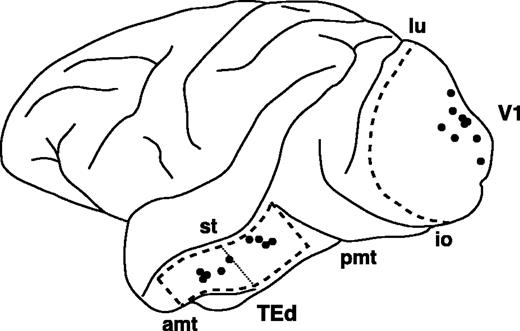
The approximate locations of the anterograde tracer injections are indicated by dots on the schematic drawing of the macaque left hemisphere. Anterior is to the left and dorsal is at the top. Area V1 (V1) and the dorsal part of area TE (TEd) are outlined by broken lines. Two subregions, TEad (anterodorsal) and TEpd (posterodorsal) are separated at thin dotted line (see Materials and Methods for details). In the following figures, the photos and drawings of the right hemisphere of the brain have been reversed to better facilitate a comparison with the left hemisphere. Table 1 provides the details of individual injections. amt, anterior middle temporal sulcus; pmt, posterior middle temporal sulcus; st, superior temporal sulcus; lu, lunate sulcus; io, inferior occipital sulcus.

In the inferior temporal cortex, several different schemes have been proposed for area subdivisions (see e.g. Bonin and Bailey, 1947; Seltzer and Pandya, 1978; Yukie et al., 1990; Felleman and Van Essen, 1991). In this study, we followed the nomenclature proposed by Yukie et al. (1990) and modified by Saleem and Tanaka (1996). In their classification, TE is divided into dorsal and ventral subdivisions (TEd and TEv) at the dorsal bank or lip of the anterior middle temporal sulcus (Fig. 1). Our TE injections were placed in TEd. According to the other classifications, the injections would be considered to be located in cytoarchitectonic areas TE2 and TE3 of Seltzer and Pandya (1978), or in CITv and AITv of Felleman and Van Essen (1991). Some injections near the ventral lip of the superior temporal sulcus (for example, case 10 in Table 1) are possibly located in TEm of Seltzer and Pandya (1978) or in CITd and AITd of Felleman and Van Essen (1991). In addition, TEd has been further divided into the anterior and posterior subregions (TEad and TEpd) at the level of the posterior tip of the anterior middle temporal sulcus (Fig. 1), based on the differences in the afferent connections from the prelunate gyrus (Shiwa, 1987; Morel and Bullier, 1990; Yukie et al., 1990). In the present study, five BDA and one PHA-L injections were located in TEad, another four BDA and one PHA-L injections in TEpd (Table 1). In the present paper, we refer to the injected area simply as area TE, except when we compared TEad and TEpd.

Data Analysis

All sections were examined under a light microscope (Eclipse E800 or Optiphot 2; Nikon, Tokyo, Japan) equipped with bright-field illumination. Section images containing labeled axons were captured digitally at a regular spacing, using a three-CCD color video camera (DXC-950; Sony, Tokyo, Japan) and either a 4× or 10× objective; these images were assembled into photomontages (Figs 2A, 3, 5, 8) using an image analysis system (MCID; Imaging Research, Ontario, Canada). The contrast and brightness of montage images were adjusted using Photoshop graphic software (Adobe, San Jose, CA) to maximize the visibility of labeled terminal patches. Higher magnification images of the labeled boutons (Fig. 8, insets) were captured using a 100× oil-immersion objective. Bouton counts were performed using a 60× oil-immersion objective.

Figure 2.

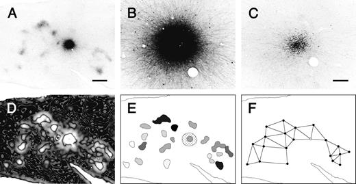
Analysis of the morphology of terminal patches. (A) The injection site and labeled patches within a tangential section was captured digitally. (B) A higher-magnification micrograph of the injection site shown in A. (C) A bundle of labeled descending axons in a section below the injection site. Such images were used to estimate the size of the injection site. (D) To determine the boundaries of labeled patches, the filtered image of the labeled section shown in A was processed with an edge-detecting method based on difference-of-Gaussian filtering. The star indicates the injection site of a different tracer, the result of which was not used in this study. (E) The reconstruction map of the patches and the injection site. The grayscale intensity of individual patches represents their relative optical density. The striped and dotted regions indicate the injection site and the halo, respectively. (F) The lines connecting the centers of the neighboring patches were determined by Gabriel graphing.

Figure 3.

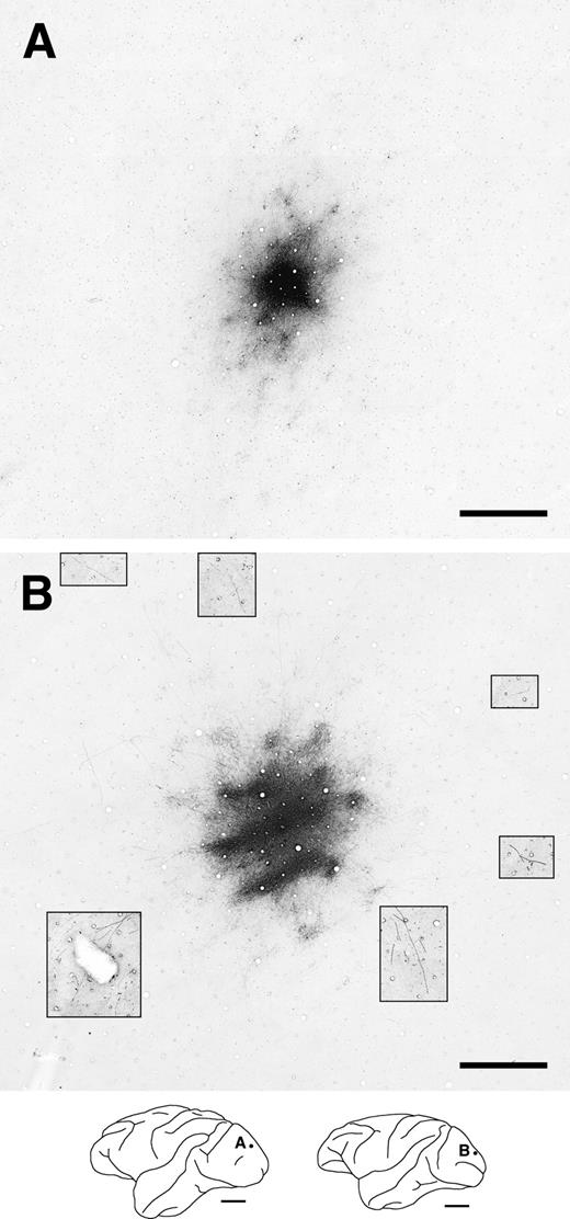
Two representative examples of labeled horizontal axons and terminal patches in tangential TE sections following BDA injections (injection size: A, 400 μm; B, 580 μm in diameter). These sections were cut primarily through layer 3. Patch-like terminal clusters are clearly visible at varying distances from the injection sites. The schematic drawings of the brain lateral view at the bottom show the locations of the photographs and injection sites as frames and dots, respectively. Scale bars: 1 mm in the photographs; 1 cm in the drawings.

The size of the injection site, the effective tracer-uptake zone by neurons, was often difficult to estimate precisely due to the presence of a densely labeled halo at the injection site (Fig. 2A,B). In sections deeper below the injection core, however, we easily found bundles of descending axons arising from neurons within the tracer-uptake zone (Fig. 2C). The bundles descend almost vertically into the white matter (Blasdel et al., 1985; Fujita and Fujita, 1996; Peters and Sethares, 1996), allowing us to estimate the size of the injection site in the upper section using the area of the descending-axon bundles in the deeper section. To compensate for the curvature of the cortex in our estimation of the size of the injection site in layers 2 and 3, we multiplied the measured area of the bundle by the expansion/contraction ratio between layer 2/3 and layer 5/6 based on the arrangement of radially penetrating large blood vessels.

The diameter of injection sites (the mean of the diameters along both the long axis and short axis) ranged from 310 to 580 μm and 230 to 350 μm in TE and V1 respectively. All of the BDA injections were used to analyze the relationship between injection size and the distribution of terminal patches. As the diameters of TE injections were somewhat larger than those for V1, to compare TE and V1 quantitatively, we used only five and four BDA injections in TE and V1, respectively, whose sizes were within a similar range of 290–400 μm (Table 1). In this data set, there were no statistical differences in the injection site sizes between TE and V1 (TE: 340 ± 22 μm, mean ± SD, n = 5; V1: 310 ± 26 μm, n = 4; Mann–Whitney U-test, P = 0.14). To study the topographical relationship between terminal patches emanating from adjacent cortical sites in TE, we made two PHA-L injections into sites adjacent to the BDA injections. PHA-L injections were used for qualitative analysis only and were not used for the quantitative analyses described above.

Terminal patches were defined as clusters of labeled axon terminals that were observed at the same position in consecutive sections accompanied by labeled axons radiating laterally from the injection site. As the patches do not exhibit clear-cut borders, we used an edge-detecting method based on difference-of-Gaussian filtering, which detects the maximal gradient in intensity of luminance in an image (Marr, 1982), to objectively determine patch boundaries. Using Photoshop software, the image of the entire section with labeled patches was processed with a median filter with a radius of 17 μm, which replaces the center value in the window with the median of all the pixel values in the window, to reduce high-spatial frequency noise, including retrogradely labeled cells and blood vessels. Images were then smoothed using a Gaussian convolution with radiuses of 75 or 120 μm to obtain two processed images. Next, the absolute values of the differences between the two Gaussian-filtered images for each corresponding pixel were calculated to create an absolute-difference image (Fig. 2D). The dark lines located within bright regions of the obtained image represent the maximal gradient in intensity of luminance in the original image (Fig. 2A). These regions corresponded well to the patch boundaries determined visually. These dark lines were delineated to create a patch-reconstruction map (Fig. 2E). In this map, the halo surrounding the injection site was delineated at an average of the maximum and minimum gray values in the section image smoothed using a Gaussian convolution with a radius of 100 μm.

After reconstruction, several parameters of the patches and injection sites, including the area, length (the diameter along the long axis), width (the diameter along the short axis), and x,y coordinates of the center, were measured using a computer image analysis program developed at the US National Institutes of Health (NIH image). Because the cortex containing the injection site was flattened before sectioning (see Materials and Methods), the section plane was almost parallel to the cortical surface around the injection site. The shape of patches was consistent across sections through layer 3, where the densest labeling of patches was observed. Therefore, we measured these parameters in one of the section through the middle of layer 3. Patches near the edges of the section were excluded from the size analysis, as the section plane was not parallel to the surface at the edge. We also excluded a number of patches merged into the halo because we could not clearly separate these sites from the halo. All measurements were made without any corrections for shrinkage and quoted as mean ± SD. The mean optical density of the patches was measured using a single section image smoothed using a median filter with a radius of 17 μm. In the reconstructed maps, each patch was shaded in grayscale according to its relative optical density (Figs 2E, 4, 6). To calculate the relative optical patch density, the difference in the mean optical density between each patch and the individual section background was normalized to this difference for the most-densely labeled patch within that section. Interpatch distances were measured from center to center between adjacent patches. Neighbors were determined by Gabriel graphing (Fig. 2F; Gabriel and Sokal, 1969), in which two points, A and B, are defined to be neighbors if the circle with a diameter of segment AB does not contain any other points.

Figure 4.

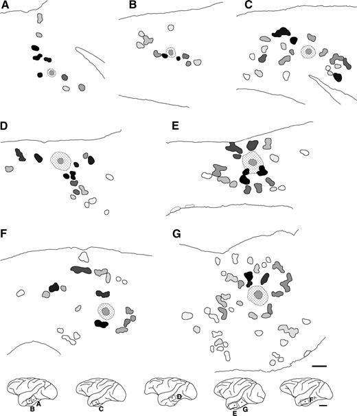
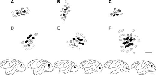
Distributions of labeled terminal patches within TE. Each schematic drawing shows an individual injection into TE. These drawings are arranged from top-left to bottom-right according to the injection size. All labeling conventions are as in Figure 2E. In the bottom row, the frames and dots indicate the locations of the patch drawings and the injection sites, respectively. Scale bars: 1 mm in the patch reconstruction maps; 1 cm in the drawings.

Results

We first describe the morphological aspects of individual patches in the dorsal part of TE (TEd). These aspects include the projection distance, spacing, size and labeling intensity of the patches. We then proceed to discuss the topographic nature of the terminal patch distributions after single or paired tracer injections. In these sections, we compare the patches in TE with those seen in V1. In addition, we compare these morphological properties of terminal patches in two subregions, the anterodorsal (TEad) and posterodosal (TEpd) parts, of TE.

Morphological Characteristics of Terminal Patches in TE and V1

Projection Distance of Patches

In two representative examples of BDA injections in tangential sections of TE cut mainly through layer 3 (Fig. 3), it is evident that, in the vicinity of the injection site, numerous labeled fibers were found extending in all directions around the injection site, forming an intense halo. A number of the labeled axons extended beyond the halo, ramifying at particular sites to form terminal clusters or ‘patches’ reported previously (Fujita and Fujita, 1996). Labeled terminal patches were visible as aggregates of labeled axon branches in layers 2 and 3. The labeling was observed across layers 2 and 3, and was densest in layer 3. Examples of reconstructed maps (see Materials and Methods) of the distribution of labeled patches originating from single injection sites (Fig. 4), including the two cases shown in Figure 3, demonstrated that patches were distributed laterally over distances of 2.5–7.7 mm from the injection sites. The number of patches resulting from a single injection ranged from 9 to 43 (19 ± 9.9, mean ± SD, n = 9 BDA injections).

In V1, labeled axons originating from an injection site also formed both a dense halo around the injection site and numerous terminal patches (Fig. 5). Although some of the labeled axons bearing boutons extended tangentially up to 4 mm in varying directions from the injection site (Fig. 5B, insets), these axons were sparse and did not form distinct clusters within a single section. In V1, distinctly clustered patches were only found within 0.9–2.0 mm of the injection site (Fig. 6). The number of patches per injection site ranged from 5 to 21 (12 ± 5.6, n = 9 BDA injections).

Figure 5.

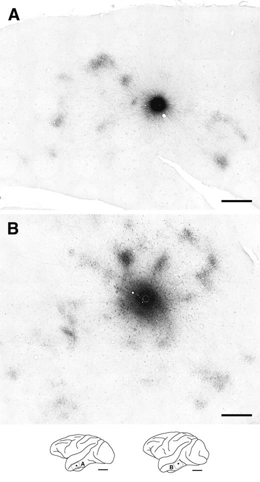
Two representative examples of intrinsic horizontal axons and terminal patches in V1. These photographs exhibit the labeled tangential sections of V1 following BDA injections (injection size: A, 250 μm; B, 350 μm in diameter). The contrast in portions of the photograph was enhanced to visualize far-reaching labeled horizontal axons (B; insets). All labeling conventions are as detailed in Figure 3.

Figure 6.

Patch distribution in V1. Each schematic drawing shows an individual V1 injection. These drawings are arranged from top-left to bottom-right according to the injection size. All conventions are as detailed in Figure 4.

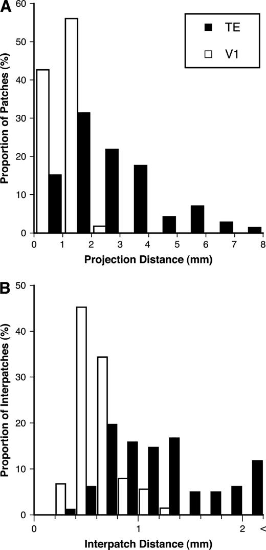
To compare the patch distributions of TE and V1, we measured the center-to-center distance from the injection site to each individual patch (projection distance; Fig. 7A). This analysis was restricted to injections of a similar size (290–400 μm in diameter) for both areas. The projection distance of patches was larger in TE than that in V1 (TE: 2.6 ± 1.6 mm, n = 74 patches for five injections; V1: 1.1 ± 0.38 mm, n = 61 for four injections; Mann–Whitney U-test, P < 0.0001). The maximum projection distance for each injection site was also larger in TE than in V1 (TE: 5.0 ± 2.0 mm, n = 5; V1: 1.6 ± 0.31 mm, n = 4; Mann–Whitney U-test, P < 0.05). These results demonstrate that horizontal axons connect to more widely distributed cortical sites in TE than those in V1.

Figure 7.

Frequency histograms of the center-to-center distances between individual patches and the injection site (A; projection distance) and between neighboring patches (B; interpatch distance) in both TE and V1.

Spacing of Patches

The interpatch distance (center-to-center distance between adjacent patches; for the definition of neighbors, see Materials and Methods) was larger in TE than in V1 (TE: 1.3 ± 0.65 mm, n = 103; V1: 0.63 ± 0.19 mm, n = 91; Mann–Whitney U-test, P < 0.0001; Fig. 7B). The coefficient of variance (CV = standard deviation/mean) of the interpatch distance was 0.51 in TE and 0.31 in V1, suggesting that the spacing between patches varied more in TE than in V1. To compare the variability of patch spacing in both areas quantitatively, we calculated the normalized absolute deviation for each spacing by taking the absolute distance of each data point from the mean for each injection and dividing this value by the mean, thus expressing the deviation as a proportion of the mean. A normalized absolute deviation close to 0 indicates that the value is close to the mean. The normalized absolute deviation for TE was larger than that for V1 (TE: 0.30 ± 0.25; V1: 0.20 ± 0.15; Mann–Whitney U-test, P < 0.01). These analyses indicate that the terminal patches emanating from a particular focal region are more irregularly spaced in TE than in V1.

Size of Patches

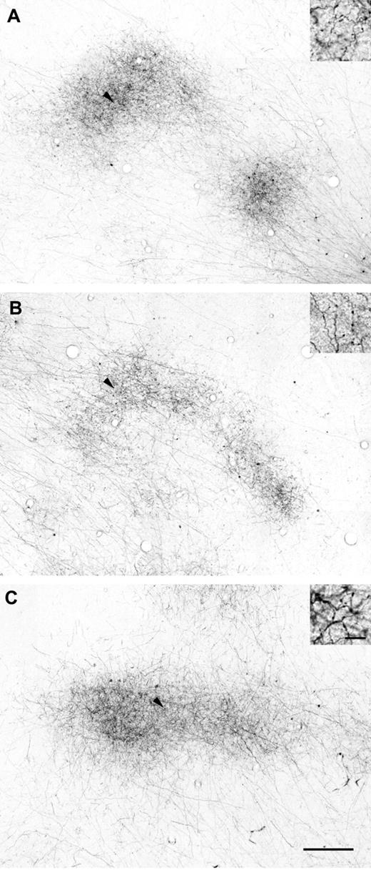
Labeled terminal patches in TE were either circular, ovoid or irregular in shape, varying significantly in size (Fig. 8A,B). A subset of patches in TE were elongated, but retained a relatively constant width (Fig. 8C). In V1, most patches were relatively constant in shape and size. For larger injections into V1, however, patches developed that were band-like and larger than other patches (Fig. 6E,F; length 1400 and 900 μm, width 350 and 340 μm respectively). As these band-like patches were positioned near the injection site (projection distance: 0.60 and 0.55 mm), these sites are likely to have been formed by the merging of multiple patches. These exceptional, atypical patches were excluded from the size analysis. Patches near the edges of the section or merged into the halo were also excluded from the size analysis because of less reliability in measurements (see Materials and Methods).

Figure 8.

Examples of terminal patches in TE at high magnification. The patches in (A) and (B) varied in size, despite emanating from the same injection. Patches occasionally aggregated to form complex shapes, likely the result of more than one overlapping patch (B). Elongated patches were frequently found following larger injections (C). The insets display higher magnification views of individual boutons within each patch, indicated by arrowheads. Scale bars: 300 μm in the photographs; 10 μm in the insets.

Both the width and length of patches were larger in TE than in V1 (Fig. 9A,B; TE: width 350 ± 71 μm, length 550 ± 180 μm, n = 60; V1: width 250 ± 57 μm, length 390 ± 93 μm, n = 57; Mann–Whitney U-test, P < 0.0001). The area of patches in TE was twice as large as that in V1 (TE: 156 000 ± 73 000 μm²; V1: 80 000 ± 29 000 μm²; Mann–Whitney U-test, P < 0.0001).

Figure 9.

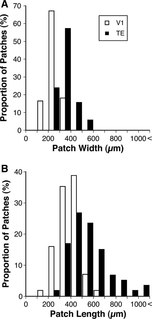
Frequency histograms of the widths (A) and lengths (B) of patches in TE and V1.

The CV of the length was somewhat larger in TE than in V1 (TE: 0.32; V1: 0.24), while the CV of the width was comparable in TE and V1 (TE: 0.20; V1: 0.23). The normalized absolute deviation of the length of patches was also larger in TE than in V1 (TE: 0.22 ± 0.17; V1 0.16 ± 0.15; Mann–Whitney U-test, P < 0.05). The normalized absolute deviation of width, however, did not exhibit any statistical differences between TE and V1 (TE: 0.14 ± 0.13; V1: 0.15 ± 0.13; Mann–Whitney U-test, P = 0.88). In TE, the normalized absolute deviation of the length was larger than that of the width. In V1, however, there were no statistical differences in the normalized absolute deviation between the length and width (Wilcoxon signed-ranks test, TE: P < 0.001, V1: P = 0.62). The results indicate that the length varied across patches in TE more than in V1, while the width of patches was relatively constant in both areas.

Relationship between Intensity of Labeling of Patches and Projection Distance

After a single BDA injection, patches exhibited varying degrees of labeling intensity in both TE and V1 (Figs 3, 5). In the patch-reconstruction maps (Figs 4 and 6), the patches are shaded in grayscale, with the degree of darkness corresponding to relative optical density. In these figures, the black patch represents the most intensely stained patch for each injection. Lighter patches, shown as close-to-white gray, are weakly labeled patches whose optical density is minimally more intense than the mean optical density of the section background. In V1, strongly labeled patches surrounded the injection site, while labeling intensities became increasingly weaker in more distant patches (Fig. 6). In TE, this tendency was less obvious, as some strongly labeled patches were observed in regions distal to the injection site, beyond other weakly labeled patches (Fig. 4).

The labeling distribution pattern in V1 and TE was quantified in plots of the relative optical density of patches against their projection distance (Fig. 10). For each graph, different symbols represent data from different injections. In V1, the optical density of patches steeply declined with increasing projection distance (Fig. 10B). In TE, the optical density also tended to decrease with projection distance, but the decreasing trend was not consistent; patches with comparable labeling intensity occurred at varying distances from the injection site (Fig. 10A). In seven of the nine injections of TE and eight of the nine injections of V1, we observed a negative correlation between patch optical density and projection distance (Spearman rank correlation test, P < 0.05). In the cases of similarly sized injections (290–400 μm in diameter), the Spearman's correlation coefficient, r_S, was lower in TE than in V1 (TE: r_S −0.65 ± 0.23, n = 5; V1: r_S −0.90 ± 0.057, n = 4; Mann–Whitney U-test, P < 0.05). The results described above indicate that patchy horizontal connections between closely spaced sites tended to be denser in both areas. In TE, however, the correlation between the density of horizontal connections and the projection distance was weaker than that in V1.

Figure 10.

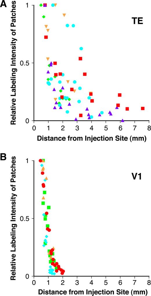
Plots of the relative patch labeling density as a function of projection distance in TE (A) and V1 (B). A relative labeling density of 1 indicates the optical density of the most intensely labeled patches for each injection. A labeling optical density of 0 is equivalent to the background optical density of the section. Different symbols represent data from different injections.

Axons within patches were studded with numerous boutons (insets in Fig. 8). To examine the correlation between bouton density and patch optical density, we counted the number of boutons per patch for the two cases in TE and the two cases in V1 shown in Figures 3 and 5. A 50 × 50 μm counting box was placed at an arbitrary position within each patch in labeled sections, and both the number of boutons and the mean optical density were then measured within the counting box. Linear regression analysis demonstrated a statistically significant correlation between the two values in the four cases examined (R² ranged from 0.66 to 0.92, P < 0.005), indicating that the measured optical density represents the approximate bouton density within the patches.

Topography of Distribution of Terminal Patches in TE and V1

Anisotropic Distribution of Patches

The overall distribution of patches surrounding each injection site was anisotropic in TE, particularly for smaller injections (Fig. 4). Following small injections, patches tended to aggregate, spreading primarily along preferred axes (Fig. 4A–D). Larger injections, however, tended to produce patches distributed over a widespread area (Fig. 4E–G). Particularly for smaller injections, the overall distribution of patches in V1 was elongated along a single axis (Fig. 6A–C) as reported (Lund et al., 1993; Malach et al., 1993; Yoshioka et al., 1996). As in TE, larger injections into V1 produced patches spreading in a more widespread direction from the injection site (Fig. 6E,F).

To estimate the axial bias for this patch distribution, we calculated the distribution anisotropy index (DAI). A labeled section was partitioned into four quadrants with the injection site as the center to maximize the number of patch centers within the two diagonal quadrants (shaded area in Fig. 11A). The ratio of the number of patches in the diagonal quadrants to the total number of patches was defined as the DAI. A DAI value close to 1 indicates that most patches were distributed along one of the axes, while a DAI value close to 0.5 indicates that the patches were distributed evenly around the injection site. In TE, the DAI was 0.82 ± 0.15 (n = 9), correlating negatively with injection size (Fig. 11B; linear regression analysis, R² = 0.69, P < 0.005). In V1, the DAI of 0.77 ± 0.11 (n = 9) also correlated negatively with the size of the injection (Fig. 11B; linear regression analysis, R² = 0.54, P < 0.05). These results indicate that the distribution of patches emanating from a focal cortical region is anisotropic in both areas. For similarly sized injections, the DAI was larger in TE than in V1 (TE: 0.89 ± 0.075, n = 5; V1: 0.70 ± 0.036, n = 4; Mann-Whitney U-test, P < 0.05), indicating that the distribution of patches emanating from a similarly sized focal region is more anisotropic in TE than in V1.

Figure 11.

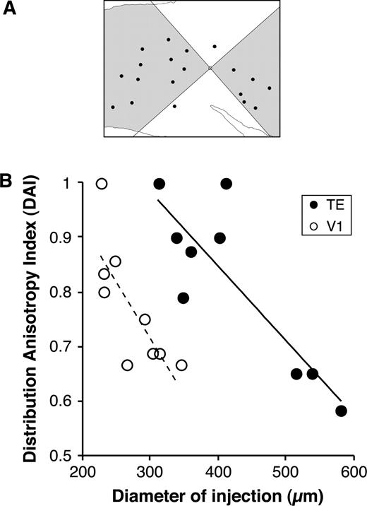
Anisotropy of patch distribution in TE and V1. (A) The distribution anisotropy index (DAI) of 0.9 was calculated as the proportion of total patches within two diagonal quadrants along the preferred axis (shaded area). (B) The relationship between the DAI and injection size (diameter). The solid and dashed lines in the graph show the linear regression lines with statistical correlation (P < 0.05).

We also evaluated the biased spread of patches by comparing the calculated anisotropy ratio to that used in previous studies (Malach et al., 1993, Fujita and Fujita, 1996; Yoshioka et al., 1996). To calculate the anisotropy ratio, we drew a rectangle that included all patch centers and maximized the ratio of the rectangle length to the width. The maximum ratio was taken as the anisotropy ratio of the overall spread of patches. In TE, the anisotropy ratio was 2.1 ± 0.54 (n = 9), a value comparable to that reported in a previous study (1.6 for one injection case: Fujita and Fujita, 1996). In V1, the anisotropy ratio was 2.1 ± 0.81 (n = 9), which was also comparable to values estimated in previous studies (1.69 ± 0.211 in Malach et al., 1993; 1.78 ± 0.68 in Yoshioka et al., 1996). For similarly sized injections, we could not observe a statistical difference in the anisotropy ratios for TE and V1 (TE: 2.3 ± 0.28, n = 5; V1: 1.6 ± 0.71, n = 4; Mann–Whitney U-test, P = 0.14). As the anisotropy ratio is easily affected by the existence of a small number of distant patches, any differences in this ratio may have been obscured.

Distribution of Patches Emanating from Adjacent Cortical Sites in TE

Injections of larger volumes of tracer demonstrated lower anisotropy in the patch distribution for both TE and V1. One potential explanation for this result is that the sets of patches originating from adjacent cortical sites are arranged along different axes. To examine this hypothesis in TE, we performed paired injections of two tracers, BDA and PHA-L, into adjacent cortical sites within TE. The paired injections were performed at anterior and posterior parts of TE within one hemisphere (Fig. 12A). The center-to-center distance between the paired BDA- and PHA-L-injection sites was 540 and 620 μm in the anterior and posterior injection cases respectively. A series of tangential sections was examined for both BDA- and PHA-L reactivity (Fig. 12B,C). The BDA-labeled (upper left) and PHA-L-labeled (lower right) patches were visualized as brown and black reaction products respectively. A series of adjacent sections was examined for BDA staining alone to verify the specific labeling of patches by the tracer. A single-stained adjacent section taken from the same location as Figure 12C includes only the BDA-labeled patch, visualized as a black reaction product (Fig. 12D).

Figure 12.

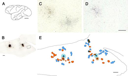
Segregation of horizontal projections from adjacent cortical sites in TE. (A) The locations of paired injections of BDA (orange) and PHA-L (blue) on the lateral view of the brain. The frame indicates the approximate location of the photograph in B. (B) Double staining of BDA- and/or PHA-L-labeled horizontal axons in a tangential section. (C) High-power view of the patches within the frame in B. The BDA- and PHA-L-labeled terminal patches were visualized as brown (top left) and black (bottom right) reaction products, respectively. (D) The adjacent section was stained for BDA labeling alone, giving a black reaction product. (E) Schematic drawing of BDA- and/or PHA-L-labeled patches in the tangential section shown in B. The orange represents BDA-labeled patches, while blue represents patches labeled by PHA-L. The regions in which the two labels overlapped are shaded with both orange and blue. The striped region indicates the injection site. Light blue and light orange indicate the individual injection haloes. Scale bars: 1 cm in A; 1 mm in B and E; and 300 μm in C and D.

The distribution of BDA- and PHA-L-labeled patches in a tangential section (Fig. 12E, shown in orange and blue respectively) demonstrated that, for an anteriorly placed injection (Fig. 12E, left), the two sets of patches were distributed along different axes of elongation. The majority of BDA-labeled patches (orange) were distributed anteriorly or posteriorly to the injection, while PHA-L-labeled patches (blue) were less anisotropic, expanding dorsoventrally from the injection. Only a few of the BDA- and PHA-L-labeled patches adjoined, while none overlapped with each other. For the posterior injection (Fig. 12E, right), the BDA- and PHA-L-labeled patches were distributed along an anteroposteriorly elongated field. In this case, a small portion of the BDA- and PHA-L-labeled patches adjoined or overlapped with each other; others were separated. These results indicate that sets of terminal patches emanating from adjacent cortical sites in TE are primarily independent; the axis of anisotropic patch distribution varies between adjacent sites.

Comparisons of Terminal Patches between TEad and TEpd

The area examined in this study includes at least two subregions, anterodorsal (TEad) and posterodorsal (TEpd) parts of TE according to Yukie et al. (1990) (Fig. 1; see Materials and Methods for details). To examine differences, if any, in anatomical properties of terminal patches between the two subregions, we divided the data of TE with respect to the location of their injection sites (Table 1) and carried out statistical analysis. The data from one injection near the border (case 1), and patches near the edges of the section or merged into the halo were excluded from the analysis. We found slight, but statistically significant, differences in patch size between these two subregions (Mann–Whitney U-test, P < 0.05): the width (TEad: 370 ± 77 μm, n = 61; TEpd: 340 ± 71 μm, n = 74), length (TEad: 650 ± 230 μm, n = 61; TEpd: 560 ± 180 μm, n = 74), area (TEad: 192 000 ± 92 000 μm², n = 61; TEpd: 154 000 ± 77 000 μm², n = 74) of patches. There was no difference in the other morphological aspects which we reported above. This provides further evidence for a progressive increase of patch size along the ventral visual pathway (Amir et al., 1993; Lund et al., 1993).

Discussion

This study quantitatively demonstrated the differences in the organization of horizontal axons in layers 2 and 3 between TE and V1, revealing some novel features of these connections in both areas. The size and spacing of terminal patches were more variable in TE than in V1. The optical density of patches exhibited a greater correlation with projection distance in V1 than in TE. There is a conspicuous anisotropy in the distribution of patches emanating from a focal cortical region in TE. In addition, the sets of patches emanating from adjacent cortical sites do not significantly overlap within TE.

Spread of Horizontal Axons

We observed labeled terminal patches at distances up to 8 mm from the injection site within the dorsal part of TE. Some of these distant patches may be formed by extrinsic projections, as several subdivisions are proposed to exist even within the dorsal part of TE on the basis of cytoarchitectonic criteria and connectivity to other cortical areas (Seltzer and Pandya, 1978; Shiwa, 1987; Morel and Bullier, 1990; Yukie et al., 1990). After injection into the posterior TE, we often found a small number of terminal patches in the anterior part of TE (data not shown). These anterior patches were separated from the patches surrounding the injection site; a subset of these patches was labeled in layers 2 and 3 as well as layer 4. These remote patches were excluded from the analysis. All of the patches examined were accompanied by horizontally projecting axons that extended through layers 2 and 3, terminating mainly in these layers.

Due to the physiological characteristics of TE neurons, visual stimulation with an object activates multiple cortical sites across a large portion of TE. TE neurons have large receptive fields which extend 15–40° or more, almost always including the fovea; these fields often overlap with each other (Gross et al., 1972; Desimone et al., 1984; Tanaka et al., 1991). TE neurons respond selectively to a particular combination of features of objects, not to the entire set of features constituting the image (Desimone et al., 1984; Tanaka et al., 1991). The widespread horizontal connections in TE may play a role in the convergence and divergence of visual signals among different sites within TE to represent the whole configuration of an object.

The majority of terminal patches within V1 were located within 2 mm (mean 1.5 mm) of the injection site, as observed in previous studies (Rockland and Lund, 1983; Blasdel et al., 1985; McGuire et al., 1991; Amir et al., 1993; Yoshioka et al., 1996). The extent of the spread of horizontal projections in V1 is thought to be comparable to the diameter of the ‘cortical point image’ (McIlwain, 1986), the cortical region activated by visual stimulation of a single retinal point (Hubel and Wiesel, 1974; Blasdel et al., 1985; LeVay, 1988; Amir et al., 1993). This hypothesis suggests that the patchy horizontal projections in V1 interconnect regions with overlapping receptive fields. A number of horizontal axons in V1, however, extended as much as 4 mm without forming clear patches. Recent studies also revealed the extension of such horizontal axons to be >2 mm (Angelucci et al., 2002; Stettler et al., 2002). These long horizontal axons in layers 2 and 3 are thought to connect neurons with nonoverlapping receptive fields, as the projection distance of these axons are beyond the point image size at ∼5° eccentricity (Hubel and Wiesel, 1974; Dow et al., 1981; Van Essen et al., 1984) where our injections were placed, according to the retinotopic map of macaque V1 (Daniel and Whitteridge, 1961; Van Essen et al., 1984; Tootell et al., 1988). These axons may provide the neural structure for the spatial interactions between regions extending beyond the classical receptive field (Gilbert et al., 1996).

Size and Spacing of Terminal Patches

In TE, the size of the labeled patches (length 0.54 ± 0.17 mm, width 0.34 ± 0.07 mm, mean ± SD) was comparable both to the tangential size of neuron clusters with similar stimulus selectivity (0.4 ± 0.2 mm), as estimated by unit recordings (Fujita et al., 1992), and to the size of active spots measured in optical imaging studies (length 0.62 ± 0.55 mm, width 0.53 ± 0.15 mm in Wang G et al., 1998; length 0.50 ± 0.13 mm, width 0.35 ± 0.09 mm in Tsunoda et al., 2001). This coincidence reinforces the close relation between terminal patches and functional domains in TE (Fujita and Fujita, 1996). The length and spacing of patches varied more in TE than in V1. In optical imaging studies (Wang G et al., 1998; Tsunoda et al., 2001), the presentation of a single visual stimulus evoked multiple TE optical spots, whose size varied more in length than in width and whose spacing appeared to be irregular. This result suggests that both the horizontal connections and the functional architecture are more irregular in TE than in V1. Optical imaging studies of TE exhibited elongated cortical regions in which optical spots shifted gradually along the cortical surface as the stimulus face was rotated in depth (Wang G et al, 1998). These regions measured up to 1 mm in length. In this study, we found multiple elongated patches in TE (Fig. 8) whose length measured 1 mm or more (Fig. 9). This horizontal projection structure could allow an elongated cortical region in which some features of an object are continuously mapped to share common inputs from a focal region in TE.

Previous studies showed that the size of terminal patches is correlated with the diameter of the basal dendritic field of layer 3 pyramidal cells in different visual areas including V1 (Lund et al., 1993; Elston and Rosa, 1998). Although there is no study directly showing the size of basal dendritic field in TE, we estimated that value from a previous study (Elston et al., 1999) in which the authors illustrated a typical example of layer 3 pyramidal cells in areas TEad of Yukie et al. (1990) and TEa of Seltzer and Pandya (1978). The estimated diameter of that cell (390 μm) is reasonably consistent with the width of patches in TEad reported in this study (370 ± 77 μm). However, it is worth noting that a number of patches were elongated, up to ∼1 mm in length, in TE, while most of the pyramidal cells in layer 3 of extrastriate areas have what appears to be a circular basal dendritic field in the tangential plane (Elston and Rosa, 1998). The elongated patches in TE may be formed by the merging of multiple circular patches deriving from different arbors.

In V1, the size and spacing of labeled patches remained relatively constant. The center-to-center distance between patches (mean 630 μm) was approximately twice as large as the average of the width and length of patches (mean 320 μm), indicating that patches are regularly separated by one patch width. The periodic pattern of horizontal connections likely arises from the functional architecture of V1, because the functional domains such as orientation columns, ocular-dominance columns, and cytochrome oxidase-rich blobs appear periodically and horizontal axons in V1 connect to domains with similar functional properties (Livingstone and Hubel, 1984; Ts'o and Gilbert, 1988; Malach et al., 1993; Yoshioka et al., 1996).

Density of Horizontal Connections and Projection Distance

In TE and V1, we observed variability in the patch labeling intensities, indicating that the density of horizontal connections between the injection site and the patches is not uniform. In TE, densely labeled patches were located both near injection sites and in distant sites. The density of horizontal connections depended less on the cortical distance in TE than in V1. As there is neither a retinotopic map nor a continuous or ordered map for the stimulus parameters in TE (Desimone and Gross, 1979; Fujita et al., 1992), it is unlikely that the cortical distance in TE represents the distance in a feature space for object representation.

Given the correspondence of patch size and the spacing between terminal patches and clusters of neurons with similar stimulus selectivity (Fujita et al., 1992), the observation that clustered horizontal connections originate primarily from pyramidal cells in TE (Tanigawa et al., 1998) leads to the expectation that neurons connected via horizontal axons in TE share certain response properties. In addition, the density of horizontal connections probably affects the similarity of stimulus selectivity between neurons at these sites. Our recent study using optical imaging and anatomical tracing techniques, however, revealed that horizontal axons in layers 2 and 3 of TE can project to sites with different response properties, in addition to those having similar properties (Tanigawa et al., 2004). We are currently investigating the general patterns governing the functional specificity of horizontal connections in TE (Fujita, 2002) and the relationship of the density of horizontal connections to the specificity.

In V1, patches with higher optical density were typically found closer to the injection site. As V1 is retinotopically organized, even within a cortical point image, closely spaced cortical sites usually represent visual fields with greater overlap. This result suggests that visual stimulation of a single retinal point can simultaneously activate neurons with similar receptive field properties at closely spaced sites within V1. Given that in V1 most horizontal axons link sites with similar receptive field properties, the accumulation of axon terminals in patches in V1 may occur via Hebbian mechanisms, based on the correlated activation of neurons with similar response properties (Stent, 1973; Changeux and Danchin, 1976; LeVay 1988).

Anisotropy in Horizontal Connections

We observed an anisotropy of horizontal projections in TE and V1; patches in both of these regions tended to aggregate along preferred axes. Although such anisotropy in V1 can be explained by the anisotropy of visual field representation (see below), in TE, where no retinotopic organization exists, this is not the case (Desimone and Gross, 1979). Given that patch regions share intracortical projections from a focal cortical region, the distribution of a group of patches in an anisotropic manner may represent a functional group related to the processing of specific visual information. In addition, we observed the projection of horizontal axons from adjacent cortical sites in TE to markedly distinct sets of cortical sites distributed along different axes. Such organization may allow a region of adjacent cortical sites to receive horizontal projections from widely distributed sites, in contrast to a simpler organization in which adjacent cortical sites project to adjacent patches. This organization may be suitable for the convergence and divergence of variable visual information among cortical sites within TE.

The distribution of terminal patches in the macaque V1 elongates perpendicular to ocular dominance stripes (Amir et al., 1993; Lund et al., 1993; Yoshioka et al., 1996). This elongation has been suggested to relate to the anisotropy of the visual field cortical representation, imposed by the interdigitating ocular dominance stripes (Amir et al., 1993; Grinvald et al., 1994; Yoshioka et al., 1996). In this study, the distribution pattern of patches following smaller injections into V1 also exhibited this tendency. Larger injections, however, produced patches distributed more isotropically around the injection, as observed in a previous study (Amir et al., 1993). Additionally, larger injections tended to produce band-like terminal patches near the injection site in V1 (Fig. 6E,F). These findings suggest that the axis of elongation of horizontal projections is gradually rotated as the injection site shifts to an adjacent location (Mitchison and Crick, 1982; Amir et al., 1993).

There are a number of possible explanations for such rotation of the axis. If an injection is positioned at a curved region of the ocular dominance stripes, the axes perpendicular to the ocular dominance stripes may vary even within the region of the injection, particularly for larger injections. In addition, the elongation of the overall patch distribution may not be strictly perpendicular to the ocular dominance stripes. In the V1 of tree shrews and new world monkeys, horizontal projections are elongated along an axis of the visual field map that corresponds to the preferred orientation of their origins (Bosking et al., 1997; Sincich and Blasdel et al., 2001). Although evidence of such axial specificity of horizontal connections related to orientation preference has not been obtained in macaques, this kind of connectional specificity, if it exists, may affect both the anisotropy of horizontal projections and the bias perpendicular to the ocular dominance stripes.

Conclusions

The present study provides quantitative evidence that the horizontal connections of TE and V1 are organized in markedly different manners. The area-specific characteristics of the horizontal connections may reflect differences in the mechanisms of intracortical information processing between TE and V1. The results correlate well with recent findings, suggesting that neocortical areas differ significantly in the anatomical features of the constituent neurons (Elston, 2002).

We thank Hisayuki Ojima for advice on double-staining techniques using BDA- and PHA-L, Kathleen S. Rockland and Yoshio Hata for advice on PHA-L labeling. We also appreciate the valuable comments of Kathleen S. Rockland and Rajagopalan Uma Maheswari on this manuscript. One of the monkeys used was obtained through the Cooperation Research Program of the Primate Institute, Kyoto University. This work was supported by grants to I.F. from Core Research for Evolutional Science and Technology (CREST) of Japan Science and Technology Corporation, and from the Ministry of Education, Science, Sports and Culture, Japan (09268222, 10164233, and 13308046). H.T. was supported by the Japan Society for the Promotion of Science Research Fellowship for Young Scientists (1300636).

Author notes

1Department of Cognitive Neuroscience, Osaka University Medical School, Suita, Osaka, 565-0871, 2Core Research for Evolutional Science and Technology, Japan Science and Technology Corporation, Toyonaka, Osaka, 560-8531, Japan and 3Laboratory for Cognitive Neuroscience, Graduate School of Frontier Biosciences, Osaka University, Toyonaka, Osaka, 560-8531, Japan