


Abstract
Container-based cloud applications require sophisticated auto-scaling methods in order to operate under different workload conditions. The choice of an auto-scaling method may significantly affect important service quality parameters, such as response time and resource utilization. Current container orchestration systems such as Kubernetes and cloud providers such as Amazon EC2 employ auto-scaling rules with static thresholds and rely mainly on infrastructure-related monitoring data, such as CPU and memory utilization. This paper presents a new dynamic multi-level (DM) auto-scaling method with dynamically changing thresholds, which uses not only infrastructure, but also application-level monitoring data. The new method is compared with seven existing auto-scaling methods in different synthetic and real-world workload scenarios. Based on experimental results, all eight auto-scaling methods are compared according to the response time and the number of instantiated containers. The results show that the proposed DM method has better overall performance under varied amount of workloads than the other auto-scaling methods. Due to satisfactory results, the proposed DM method is implemented in the SWITCH software engineering system for time-critical cloud applications.
1. INTRODUCTION
Cloud computing as a pay-per-use on-demand offer has become a preferable solution for providing various types of CPU, memory and network-intensive applications over the Internet. These include finite element analysis [1], video streaming, gaming, early warning systems and various other Internet of Things (IoT) time-critical applications.
Achieving favourable quality under the conditions of dynamically varying workload intensity is essential for such applications in order to make them useful in a business context. Taherizadeh et al. [2] studied a range of quality metrics that can be obtained by advanced cloud monitoring systems and can be used to achieve high operational quality. For example, applications’ quality can be quantitatively measured by response time and resource utilization aspects.
As the workload becomes more dynamic and varies over time, using the lightweight container-based virtualization can support adaptation improvements on both application performance and resource utilization aspects faster and more efficiently than using VMs [3]. This work uses container-based virtualization technology, particularly Docker1 and CoreOS2 for the delivery of applications in the cloud. Despite container technologies’ potential, capabilities for auto-scaling cloud-based applications [4–11] can still be significantly improved. Inadequate auto-scaling that is unable to address changing workload intensity over time results in either resource under-provisioning—in which case the application suffers from low performance—or resource over-provisioning—in which case the utilization of allocated resources is low. Therefore, adaptation methods are required for fine-grained auto-scaling in response to dynamic fluctuations in workload at runtime.
Many existing auto-scaling mechanisms use rules with fixed thresholds, which are almost exclusively based on infrastructure-level metrics, such as CPU utilization. This includes auto-scaling methods employed by commercial VM-based cloud providers such as Microsoft Azure3 and Amazon EC2,4 and open-source container orchestrators such as Kubernetes5 and OpenShift Origin.6 Although such methods may be useful for some basic types of cloud applications, their performance and resource utilization drops when various CPU, memory and network-intensive time-critical applications need to be used [12].
The hypothesis of the present work is that the use of high-level metrics and dynamically specifying thresholds for auto-scaling rules may provide for more fine-grained reaction to workload fluctuations, and thus it can improve application performance and a higher level of resource utilization. The goal of this paper is, therefore, to develop a new dynamic auto-scaling method that automatically adjusts thresholds depending on the execution environment status observed by advanced multi-level monitoring systems. In this way, multi-level monitoring information that includes both infrastructure and application-specific metrics would help the service providers accomplish satisfactory adaptation mechanisms for the various runtime conditions.
The main contribution of this paper can be summarized as follows: (i) introducing a multi-level monitoring framework to meet the whole spectrum of monitoring requirements for containerized self-adaptive applications, (ii) presenting a method to define rules with dynamic thresholds which may be employed for launching and terminating container instances and (iii) proposing a fine-grained auto-scaling method based on a set of adaptation rules with dynamic thresholds.
A fine-grained auto-scaling approach continuously allocates the optimal amount of resources needed to ensure application performance with neither resource over-provisioning nor under-provisioning. Such an auto-scaling method should be able to satisfy application performance requirements (e.g. response time constraints), while optimizing the resource utilization in terms of the number of container instances, as shown in Fig. 1.
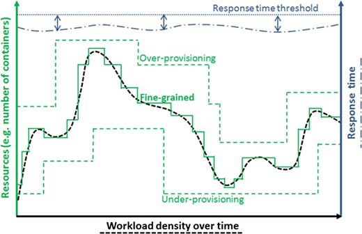
Fine-grained auto-scaling of a containerized application.
With regard to different workload patterns, it is our aim to evaluate the proposed auto-scaling method relating to its ability to support self-adaptive cloud-based applications with a varied number of requests at runtime. Additionally, it is our aim to compare the new method with seven other auto-scaling methods which are predominantly used in current software engineering practices.
The rest of the paper is organized as follows. Section 2 presents a review of related work focusing on the auto-scaling of VM and container-based applications. Section 3 describes monitoring requirements for containerized applications. Section 4 presents the architecture of the new adaptation method in detail, which is followed by empirical evaluation in Section 5. Section 6 contains a critical discussion of the proposed approach, while conclusions are presented in Section 7.
2. RELATED WORK
Cloud applications and systems with auto-scaling properties have been discussed in experience studies and are contained in various commercial solutions. This section presents a review of important auto-scaling methods as summarized in Table 1. The similarities and differences among the presented auto-scaling approaches offer an opportunity for comprehensive conception of the term ‘elasticity’ within cloud-based applications. The proposed new method called dynamic multi-level (DM) auto-scaling is also shown for completeness in the last row of Table 1.
Overview of various auto-scaling approaches for cloud applications.
| Paper | Virtualization technology | Infrastructure-level metrics | Application-level metrics | Technique | Adjustment ability |
|---|---|---|---|---|---|
| Al-Sharif et al. [4] | VM | CPU, memory and bandwidth | Nothing | Rule-based | Static |
| Islam et al. [5] | VM | CPU | Response time | Linear regression and neural networks | Static |
| Jamshidi et al. [6] | VM | CPU, memory, etc | Response time and application throughput | Reinforcement learning (Q-Learning) | Dynamic |
| Arabnejad et al. [7] | VM | Nothing | Response time and application throughput | Fuzzy logic control and reinforcement learning | Dynamic |
| Tsoumakos et al. [8] | VM | CPU, memory, bandwidth, etc | Response time and application throughput | Reinforcement learning (Q-Learning) | Static |
| Gandhi et al. [9] | VM | CPU | Response time and application throughput | Queueing model and Kalman filtering | Dynamic |
| Baresi et al. [10] | Container | CPU and memory | Response time and application throughput | Control theory | Dynamic |
| Horizontal Pod Auto-scaling (HPA) used by Kubernetes | Container | CPU | Nothing | Rule-based | Static |
| Target Tracking Scaling (TTS) and Step Scaling (SS) used by Amazon | VM and container | CPU and bandwidth | Application throughput | Rule-based | Static |
| THRESHOLD (THRES) [11] | VM and container | CPU | Nothing | Rule-based | Static |
| Multiple Policies (MP) used by Google | VM | CPU | Application throughput | Rule-based | Static |
| DM | Container | CPU, memory and bandwidth | Response time and application throughput | Rule-based | Dynamic |
2.1. Experience studies
Al-Sharif et al. [4] presented a framework called ACCRS (Autonomic Cloud Computing Resource Scaling) to provision a sufficient number of VMs in order to meet the changing resource needs of a cloud-based application. The proposed adaptation approach uses a set of fixed thresholds for CPU, memory, and bandwidth utilization to evaluate states of resources at runtime. The workload can be identified as a heavy or lightweight if any of these attributes violate the thresholds. Their resource scaling framework applies a single-level monitoring system which measures only infrastructure-level metrics, and hence the service response time or application throughput does not have any role in determining the auto-scaling actions.
Islam et al. [5] developed proactive cloud resource management in which linear regression and neural networks have been applied to predict and satisfy future resource demands. The proposed performance prediction model estimates upcoming resource utilization (e.g. an aggregated percentage of CPU usage of all running VM instances) at runtime and is capable of launching additional VMs to maximize application performance. In this approach, only CPU utilization is used to train a prediction model, and their approach does not include other types of resources, e.g. memory. The authors propose using a 12-minute prediction interval, because the setup time of VM instances in general is around 5–15 minutes. This low rate of prediction is not suitable for continuously changing workloads. Moreover, in such proactive methods [13–16], for each workload change, it takes too long to converge towards a stable driven performance model, and thus the application may provide poor quality of service (QoS) to the users during the first stages of the learning period.
Jamshidi et al. [6] presented a self-learning adaptation technique called FQL4KE to perform scaling actions in terms of increment or decrement in the number of VMs. FQL4KE applies a fuzzy control method based on a reinforcement learning algorithm. However, in some real-world environments, the number of situations is enormous, and therefore the reinforcement learning procedure may take too long to converge for any new change in the execution environment. Therefore, using reinforcement learning may become impractical due to the time constraints imposed by time-critical applications such as early warning systems.
Arabnejad et al. [7] proposed a fuzzy auto-scaling controller which can be combined with two reinforcement learning approaches: (i) fuzzy SARSA learning (FSL) and (ii) fuzzy Q-learning (FQL). In this work, the monitoring system collects required metrics such as response time, application throughput and the number of VMs in order to feed the auto-scaling controller. The auto-scaling controller automatically scales the number of VMs for dynamic resource allocations to react to workload fluctuations. It should be noted that the proposed architecture is usable only for a specific kind of virtualization platform called OpenStack. Moreover, the controller has to select scaling actions among a limited number of possible operations. That means if a drastic increase suddenly appears in the workload intensity, the proposed auto-scaling system is able to add just one or two VM instances that perhaps cannot provide enough resources to maintain an acceptable QoS.
Tsoumakos et al. [8] introduced a resource provisioning mechanism called TIRAMOLA to identify the number of VMs needed to satisfy user-defined objectives for a NoSQL database cluster. The proposed approach combines Markov decision process (MDP) with Q-learning as a reinforcement learning technique. It continuously decides the most advantageous state which can be reached at runtime, and hence identifies available actions in each state that can either add or remove NoSQL nodes, or do nothing. The rationale of TIRAMOLA is acting in a predictable manner when the regular workload pattern can be identified. Therefore, previously unseen workloads are the main barrier to quick adaptation of the entire system to address the performance objective of interactive services. Moreover, TIRAMOLA is limited to the elasticity of a certain type of application like NoSQL databases. Besides this, the monitoring part should collect client-side statistics in addition to server-side metrics (e.g. CPU, memory and bandwidth, query throughput, etc.). To this end, clients need to be modified so that each one can report its own statistics, which is not a feasible solution for many use cases.
Gandhi et al. [9] presented a model-driven auto-scaler called dependable compute cloud (DC2) which proactively tends to ensure application performance to meet user-specified requirements. The proposed approach applies a combination of a queueing model and the Kalman filter technique to produce estimations of the average service time at runtime. The functionality of DC2 is focused on preventing resource under-utilization, and hence it may cause an over-provisioning issue during execution time. Furthermore, the Kalman filter process is iteratively continued at every 10-s monitoring interval, it needs some time (e.g. few minutes) to calibrate the driven model based on the monitoring data for every new state. Accordingly, the challenge in this regard is that the accuracy of the proposed auto-scaling approach may decrease for special workload patterns such as a new, drastically changing scenario over time.
Baresi et al. [10] presented an auto-scaling technique that uses an adaptive discrete-time feedback controller to enable a containerized application to dynamically scale resources, both horizontally and vertically. Horizontal scaling means the addition or removal of container instances, while vertical scaling represents expanding or shrinking the amount of resources allocated to a running container. In this work, a component called ECoWare agent should be deployed in each VM. An ECoWare agent is responsible for the collection of container-specific monitoring data, such as containers’ utilization of CPU, memory, and so on. This component is also in charge of launching or terminating a container in the VM, or changing the resources allocated to a container.
2.2. Production rule-based solutions
Currently, many commercial cloud providers (e.g. Amazon EC2 and Google Cloud Platform), as well as container management systems (e.g. Kubernetes), provide static rule-based auto-scaling approaches which are not flexible enough to adjust themselves to the runtime status of the execution environment. In this subsection, we explain some important rule-based auto-scaling solutions for the purpose of comparison to our proposed DM method. These solutions have been chosen for comparison to our method since they are also rule-based and considered as advanced auto-scaling approaches, and which are used in production systems.
Our goal is to evaluate the proposed DM method through a set of empirical experiments which are presented in Section 5. Figure 2 complements Fig. 1, and presents two important quality properties which are analysed by the study and lead to the definition of a fine-grained auto-scaling approach.
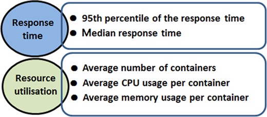
Important quality properties of cloud-based applications and associated metrics.
Generally, a typical practice in current commercial services is to use fixed, single-level scaling rules. For example, it is possible to specify a CPU-based auto-scaling policy that more VMs/containers should be launched if the average CPU utilization is over a fixed threshold such as 80%; while some VMs/containers may be terminated if the average CPU utilization is less than 80%. These settings cannot be very useful for special workload patterns such as drastically changing scenarios. Moreover, they lead to a stable system at 80% resource utilization, which means 20% of resources are wasted, which is not desirable. One of the main open challenges and significant technical issues in proposing an auto-scaling technique is to decide to what extent the adaptation approach should be self-adjustable to changes in the execution environment.
In our proposed auto-scaling method, both infrastructure-level metrics (CPU, memory, etc.) and application-specific metrics (e.g. response time and application throughput) are the factors that dynamically influence the adjustable, auto-scaling rules. Our proposed method is dynamic because it uses self-adaptive rules which are employed for launching and terminating container instances. These rules are adjusted according to the workload intensity at runtime. It means, in our approach, conditions when containers are initiated or terminated can be different and do not need to be predefined.
In the following, we proceed with an analysis of existing auto-scaling methods which are widely used and serve as means for comparison with the proposed DM method.
2.2.1. Kubernetes—horizontal pod auto-scaling
Kubernetes is a lightweight container management system able to orchestrate containers and automatically provide horizontal scalability of applications. In Kubernetes, a pod is a group of one, or a small number of containers which are tightly coupled together with a shared IP address and port space. One pod simply represents a single instance of an application that can be replicated, if more instances are needed to process the growing workload. In Kubernetes, the horizontal pod auto-scaling (HPA) approach [17] is a control loop algorithm principally based on CPU utilization; no matter how workload intensity or application performance is behaving. HPA (shown in Algorithm 1) is able to increase or decrease the number of pods to maintain an average CPU utilization across all pods close to a desired value, e.g. Targetcpu = 80%.
A SUM_Cluster is the grouping function used to calculate the total sum of the cluster. The period of the Kubernetes auto-scaler is 30 s by default, which also can be changed. At each iteration, Kubernetes’ controller increases or decreases the number of pods according to NoP as the output of the HPA algorithm.
Kubernetes HPA algorithm.
| Inputs: |
| Targetcpu: Targeted per-pod CPU resource usage |
| CLTP: Control Loop Time Period in seconds, e.g. 30 seconds |
| Outputs: |
| NoP: Number of pods to be running |
| do{ |
| Cluster = [Pod1,…, PodN]; |
| SumCpu=SUM_Cluster(cpu_usage_of_pod1,…,cpu_usage_of_podN); |
| NoP = |
| wait(CLTP); |
| } while(true); |
2.2.2. AWS—target tracking scaling
The Amazon EC2 AWS platform offers a target tracking scaling (TTS) [18] approach, which is able to provide dynamic adjustments based on a target value for a specific metric. This approach applies single-level auto-scaling rules to consider either an infrastructure-level metric (e.g. average CPU utilization) or an application-level parameter (e.g. application throughput per instance). To this end, a predefined target value must be set for a metric considered in the auto-scaling rule. Moreover, the minimum and maximum number of instances in the cluster should be specified. TTS adds or removes application instances as required to keep the metric at, or close to, the specified target value.
The default configuration in AWS is capable of scaling based upon a metric with a 5-minute frequency. This frequency can be changed to 1 minute—which is known as detailed auto-scaling option. TTS is able to increase the cluster capacity when the specified metric is above the target value, or decrease the cluster size when the specified metric is below the target value for a specified consecutive periods e.g. even one interval. For a large cluster, the workload is spread over a large number of instances. Adding a new instance or removing a running instance causes less of a gap between the target value and the actual metric data points. In contrast, for a small cluster, adding or removing an instance may cause a big gap between the target value and the actual metric data points. Therefore, in addition to keeping the metric close to the target value, TTS should also adjust itself to minimize rapid fluctuations in the capacity of the cluster.
For example, a rule specified as ‘TTS1 (CPU, 80%, ±1)’ can be executed to keep the average CPU utilization of the cluster at 80% by adding or removing one instance per scaling action. Moreover, the rule ‘TTS’ can also be used to adjust the number of instances by a percentage. For instance, a rule named ‘TTS2 (CPU, 80%, ±20%)’ adds 20% more instances or removes 20% fewer instances, if the conditions are satisfied. For example, if four instances are currently running in the cluster, and the average CPU utilization goes higher than 80% during the last minute, TTS2 determines that 0.8 instance (that is 20% of four instances) should be added. In this case, TTS rounds up 0.8 and adds one instance. Or, if in a certain condition, TTS2 decides to remove 1.5 instances, TTS can round down and stop only one instance.
2.2.3. AWS—step scaling
The step scaling (SS) [19] auto-scaling approach can also be applied in AWS. For instance, if the average CPU utilization needs to be below 80%, it is possible to define different scaling steps. Figure 3a shows the first part of an AWS auto-scaling example called ‘SS1’ to expand the capacity of the cluster, while the workload is increasing. In this example, one instance will be added for a modest breach (from 80% to 85%), two more instances will be instantiated for somewhat bigger breaches (from 85% to 95%), and four instances for CPU utilization that exceeds 95%. The ranges of step adjustments should not overlap or even have a gap. In this example, SS1 periodically calculates the 1-minute aggregated value of the average CPU utilization from all instances. Then, if this value exceeds 80%, SS1 compares it against the upper and lower bounds specified by various step adjustments to decide which action to be performed.
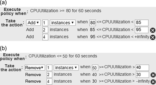
An AWS auto-scaling example named SS1.
Similarly, it is possible to define different steps to decrease the number of instances running in the cluster. As an example, Fig. 3b shows three steps to remove unnecessary instances when the average CPU utilization falls below 50%.
In AWS, step scaling policies can be also defined on a percentage basis. That means to handle a growing workload at runtime, SS is able to increase the number of instances by the percentage of cluster size. Figure 4a shows the first part of an AWS auto-scaling example called ‘SS2’ that includes two-step adjustments to increase the number of instances in the cluster by 20% and 30% of the cluster size at the respective steps. If the resulting value is not an integer, SS2 rounds this value. In this case, values greater than 1 are rounded down. Values between 0 and 1 are rounded to 1. For example, if the current number of instances in the cluster is four, adding 30% of the cluster will result in the deployment of one more instance. As such, 20% of four instances is 1.2 instances, which is rounded down to 1 instance.
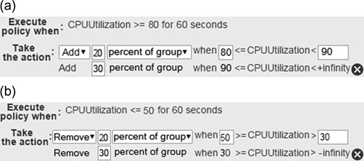
An AWS auto-scaling example named SS2.
It is also possible to define a similar set of policies to decrease the number of instances deployed in the cluster. In this way, SS2 is capable of decreasing the current capacity of the cluster by the specified percentage at different step adjustments. Figure 4b shows a two-step auto-scaling to handle a decreasing workload at runtime, and hence to reduce the number of instances in the cluster by 20% and 30% of the cluster size. The resulting values between 0 and −1 are rounded to −1. Moreover, the resulting values less than −1 are rounded up. For example, −3.78 is rounded to −3.
2.2.4. THRESHOLD
THRES (Metric, UP%, DOWN%) [11] is a static single-level auto-scaling method which horizontally adds a container instance if an aggregated metric (e.g. average CPU or memory usage of the cluster) reaches the predefined UP% threshold, and removes a container instance when it falls below the predetermined DOWN% threshold for a default number of successive intervals, e.g. two intervals. ‘THRES1 (CPU, 80%, 50%)’ is an example for such a static single-level auto-scaling method.
The ‘THRES2 (CPU, 80%, 50%, RT, 190 ms)’ method also can be defined as an example for a static multi-level provisioning approach that is also able to consider the average response time (RT). To add a new container instance, both the average resource utilization and response time thresholds (in this use case, 80% and 190 ms, respectively) should be reached for two consecutive intervals. To remove a container from the cluster, the average CPU usage of the cluster should be less than 50% during the last two periods.
2.2.5. Google—Multiple Policies
The Google Cloud Platform supports an auto-scaling mechanism called ‘MP’ to use multiple auto-scaling policies individually at different levels [20]. For example, the MP auto-scaler is able to consider two policies. One policy can be based upon average CPU utilization of the cluster as an infrastructure-level parameter. Another policy can be based on application throughput of the load-balancer (ATLB) as an application-level metric. In other words, each policy is a single-level rule that is defined and based on only one metric. MP calculates the number of necessary instances recommended by each policy, and then picks the policy that leaves the largest number of instances in the cluster. This feature conservatively ensures that the cluster always has enough capacity to handle the workload.
In this way, a target value should be defined for each metric. For example, ‘MP (CPU = 80%, ATLB = 80%)’ is a two-policy method which continuously collects the average CPU utilization of the cluster, as well as the load-balancing serving capacity. In this example, setting a 0.8 target usage tells the MP auto-scaler to maintain an average CPU utilization of 80% in the cluster. Moreover, MP will scale the cluster to maintain 80% of the load-balancing serving capacity. For instance, if the maximum load-balancing serving capacity is defined as 100 RPS (requests per second) per instance, MP will add or remove instances from the cluster to maintain 80% of the serving capacity, or 80 RPS per instance.
3. MONITORING CONTAINERIZED APPLICATIONS
In comparison to traditional monitoring approaches for datacentres, an advanced cloud monitoring system should be able to monitor various metrics at different levels, including container and application-level metrics, instead of only VM-level metrics [21–24]. When designing a new auto-scaling approach, our aim is to rely on such advanced multi-level monitoring systems as described in the following subsections.
3.1. Container-level monitoring
If the system applies container-based virtualization instead of VMs to use a lightweight mechanism for deploying and scaling services in the cloud, container-level monitoring becomes compulsory. A container-level monitoring system is able to monitor containers and display runtime value of key attributes including CPU, memory, and network traffic usage of each container instances. As listed in Table 2, there are different tools offered specifically for the purpose of monitoring containers and expose value of characteristics for a given container at runtime.
Overview of container-level monitoring tools.
| Tool | Open Source | License | Scalability | Alerting | TSDB | GUI |
|---|---|---|---|---|---|---|
| cAdvisor | Yes | Apache 2 | No | No | No | Yes |
| cAdvisorIGa | Yes | Mixed | Yes | No | Yes | Yes |
| Prometheus | Yes | Apache 2 | No | Yes | Yes | Yes |
| DUCPb | Yes | Commercial | Yes | Yes | No | Yes |
| Scout | Yes | Commercial | No | Yes | Yes | Yes |
aUsing three tools together: cAdvisor (Apache 2) + InfluxDB (MIT) + Grafana (Apache 2).
bDocker Universal Control Plane (DUCP), https://docs.docker.com/ucp/
cAdvisor7 is a system that measures, processes, aggregates and shows monitoring data obtained from running containers. This monitoring data can be applied as an awareness of the performance features and resource usage of containers over time. cAdvisor only displays monitoring information measured during the last 60 s. However, it is capable of storing the data in an external Time Series Database (TSDB) such as InfluxDB8 which supports long-term storage and analysis. Besides that, Grafana9 is a Web interface to visualize large-scale monitoring data. Using InfluxDB and Grafana on top of the cAdvisor monitoring system could significantly improve visualizing the monitored metrics in understandable charts for different time periods.
Prometheus10 is a monitoring tool which includes a TSDB. It is able to gather monitoring metrics at different intervals, show the measurements, investigate rule expressions, and trigger alerts when the system commences to experience abnormal situation. However cAdvisor is considered as the easier monitoring system to be used in comparison to Prometheus, it has restrictions with alert management. It should be noted that both may not be able to appropriately offer turnkey scalability to handle large number of containers.
DUCP is a commercial solution to monitor, deploy and manage distributed applications using Docker. Web-based user interface and high scalability are the notable characteristics of this container management solution.
Scout11 is also a container monitoring system which has a Web interface management console, and is capable of storing measured values taken during at most 30 days. This monitoring solution supports alerting based on predetermined thresholds.
3.2. Application-level monitoring
Application-level monitoring, which is an open research challenge yet, measures parameters that present information about the situation of an application and its performance; such as response time or application throughput. Table 3 shows a list of cloud monitoring systems which are able to measure application-specific metrics.
Overview of application-level monitoring tools.
| Tool | Open Source | License | Scalability | Alerting | TSDB | GUI |
|---|---|---|---|---|---|---|
| Zenoss | Yes | GPL | Yes | Yes | Yes | Yes |
| Ganglia | Yes | BSD | Yes | No | Yes | Yes |
| Zabbix | Yes | GPL | Yes | Yes | Yes | Yes |
| Lattice | Yes | Apache 2 | Yes | No | No | No |
| JCatascopia | Yes | Apache 2 | Yes | No | Yes | Yes |
Zenoss [25] is an agent-less monitoring platform based on the SNMP protocol. This tool has an open architecture to help consumers customize it based on their monitoring requirements. However, it has a limited open-source version and the full version for monitoring requires payment, so its applicability in research is undermined.
Ganglia [26] is a scalable monitoring system for high-performance computing environments such as clusters and grids. This tool is generally designed to collect infrastructure-related monitoring data about machines in clusters and display this information as a series of graphs in a web-based interface. It is not suitable for bulk data transfer due to the lack of congestion avoidance and windowed flow control in Ganglia.
Zabbix [27] which is an agent-based monitoring solution supports an automated alerting ability to trigger if a predetermined condition happens. Zabbix is mainly implemented to monitor network services and network parameters. As a disadvantage to be considered, the auto-discovery characteristic of this monitoring system can be inefficient [28]. For example for Zabbix, sometimes it may take almost five minutes to discover that a host is no longer running in the environment. This restriction in time may be a serious issue for any time-critical self-adaptation scenario.
Lattice [29], as a non-intrusive monitoring system, is mainly implemented for monitoring highly dynamic cloud-based environments, consisting of a large number of resources. The functionalities of this monitoring system are the abilities for the distribution and collection of monitoring data via either UDP protocol or multicast addresses. Therefore, the Lattice platform is not meant for automated alerting, visualization and evaluation [30].
JCatascopia [31] is a scalable monitoring platform which is capable of monitoring federated clouds. This open-source monitoring tool is designed for server/agent architecture. Monitoring Agents are able to measure whether infrastructure-specific parameters or application-level metrics, and then they send the monitoring data to a central entity called a Monitoring Server.
3.3. The SWITCH monitoring system
The SWITCH project12 provides a software engineering platform for time-critical cloud applications [12]. In order to develop a monitoring system for SWITCH, JCatascopia has been chosen as the baseline technology and was extended to be able to measure container-level metrics. Each container consists of two parts: an application instance and a Monitoring Agent. Monitoring Agents are the actual components that collect individual metrics’ values. Since JCatascopia is written in Java, each container which includes a Monitoring Agent requires some packages and a certain amount of memory for a Java virtual machine (JVM) even if the monitored application running alongside the Monitoring Agent in the container is not programmed in Java. Therefore, Monitoring Agents in the SWITCH project have been implemented through the StatsD protocol13 available for many programming languages such as C/C++ and Python. Accordingly in the SWITCH platform, a running container includes: (i) a service as application instance and (ii) a StatsD client as a Monitoring Agent.
The functioning of the SWITCH monitoring system is illustrated in Fig. 5.
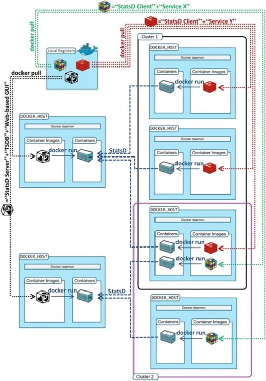
The SWITCH monitoring system.
In Fig. 5, two different container images ( and
and  ) have been pulled from a local registry, and each one provides a different scalable service, for example Service X and Service Y. Therefore, there are two different service clusters in this figure. Starting a new container instance of a given service means that the service scales up, and stopping it means that it scales down. Once a new container is instantiated, it is allocated to a logical cluster. The SWITCH monitoring system keeps track of these logical clusters for every running service. For example, Fig. 5 shows that Cluster 1 hosts three instances of Service X and Cluster 2 hosts two instances of Service Y.
The monitoring data streams coming from Monitoring Agents to the Monitoring Server via the StatsD protocol are stored in a Cassandra TSDB for the storage of series of time-ordered data points. The SWITCH web-based interactive development environment (IDE) allows all external entities to access the monitoring information stored in the TSDB in a unified way, via prepared REST-based web services, APIs and diagrams.
For the SWITCH platform, a container image ( as shown in Fig. 5) has been built to include the following three entities: (i) a StatsD server as Monitoring Server, (ii) TSDB and (iii) the SWITCH web-based IDE. This container image is open-source and publically released on Docker Hub [32]. It should be noted that it is also possible to have individual container images for every one of these three entities. The SWITCH monitoring system is freely available to researchers at GitHub [33] under an Apache 2 license.
A Docker registry which can be installed locally is used to store Docker images. Using a local registry makes it faster to pull container images and run container instances of services across cluster nodes. A local Docker registry significantly reduces deployment latency and network overhead when running containers across the spread of host machines in a region. Moreover, it may be possible to design deployment strategies that make use of cached container images, thus, further improving deployment time.
4. METHOD AND ARCHITECTURE
This study introduces a DM auto-scaling method which is included together with the SWITCH monitoring system in a functional architecture (shown in Fig. 6) for adaptive containerized applications.
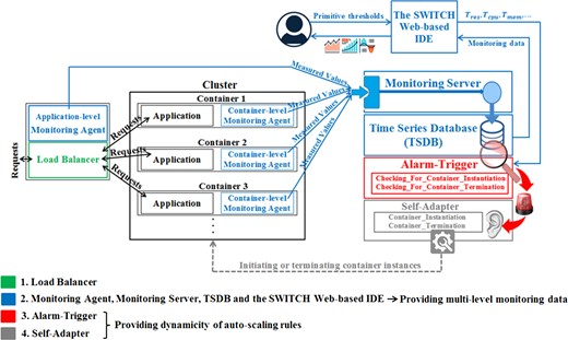
Auto-scaling architecture for adaptive container-based applications.
In our work, we consider that each host in a cluster is able to include at most one container instance per service, while one host can belong to different clusters at the same time. That means more than one container instance can be deployed on one host, but nevertheless they should provide different services. This situation is a realistic case of an operational environment where different types of services should be scaled. When a specific service is instantiated at the host, it exposes its interfaces at specific port numbers, which must not clash with the port numbers of other instantiated services. Then, it makes sense to provide an internal, so-called vertical elasticity mechanism for the allocation of CPU and memory resources to different services within the same host machine, but, it would make no sense to instantiate additional instances of the same service on the same host machine.
Generally, if two or more containers run on a host machine, by default all containers will get the same proportion of CPU cycles. In this situation, if tasks in one container are idle, other containers are able to use the leftover CPU cycles. Moreover, it is possible to modify identical proportions assigned to running containers by using a relative weighting mechanism. In such a manner, when all containers running on a host machine attempt to use 100% of the CPU time, the relative weights give each container access to a defined proportion of the host machine’s CPU cycles (since CPU cycles are limited).
When enough CPU cycles are available, all containers running on a host machine use as much CPU as they need regardless of the assigned weights. However, there is no guarantee that each container will have a specific amount of CPU time at runtime. Because the actual amount of CPU cycles allocated to each container instance will vary depending on the number of containers running on the same host machine and the relative CPU-share settings assigned to containers. To ensure that no container can starve out other containers on a single host machine, if a running container includes a CPU-bound service, other containers that will be deployed on that machine should not be identified as computationally intensive services. This principle has been adopted also for memory-intensive applications. In this work, all containers have the same weight to gain access to the CPU cycles and the same limit at the use of memory. This makes it an appropriate case of so-called horizontal scaling.
The proposed architecture includes the following components: Load-Balancer, Monitoring Agent, Monitoring Server, TSDB, Alarm-Trigger and Self-Adapter. These are explained in detail in the following subsections.
4.1. Load-Balancer
The Load-Balancer (e.g. HAProxy) provides high-availability support for containerized applications by spreading requests across multiple container instances.
4.2. Monitoring Agent, Monitoring Server, TSDB and the SWITCH Web-based IDE
The monitoring system is able to measure both container-level metrics (e.g. CPU and memory usage of containers) and application-level parameters (e.g. average response time and throughput of the application). Therefore, two types of Monitoring Agents which measure container-level and application-level metrics are included in the architecture.
The application-level Monitoring Agent is in charge of monitoring the Load-Balancer. Application-level metrics which are applied in the context of the proposed auto-scaling method are AvgRT (average response time to reply to a user’s request), AT (application throughput which means the average number of requests per second processed by one container instance), and cont (number of container instances behind the Load-Balancer).
The distributed nature of our developed agent-based monitoring system supports a fully interoperable, lightweight architecture which quenches the runtime overhead of the whole system to a number of Monitoring Agents. A Monitoring Agent which is running alongside the application in a container collects individual metrics and aggregates the measured values to be transmitted to the Monitoring Server. The Monitoring Server is a component that receives measured metrics from the Monitoring Agents. This monitoring system is able to store measured values in the Apache Cassandra server as TSDB.
When a container is launched, the Monitoring Agent will automatically send the Monitoring Server a message to register itself as a new metric stream, and then it will start collecting metrics and continuously forward the measured values to the Monitoring Server.
The SWITCH web-based IDE is also used to set primitive thresholds needed for adaptation policies. It is also a key tool used by software engineers to analyse events in a dynamically changing cloud environment.
4.3. Alarm-Trigger
The Alarm-Trigger is a rule-based component which checks the incoming monitoring data and notifies the Self-Adapter when the system is going to experience abnormal behaviour. The Alarm-Trigger continuously processes two functions. One function named checking for container instantiation (CFCI) has been defined in the Alarm-Trigger to investigate if it is needed to start new container instances. Moreover, another function named checking for container termination (CFCT) has been defined in the Alarm-Trigger to evaluate if one of the running container instances can be terminated without any application performance degradation.
An important application-level metric which is used in the operation of the Alarm-Trigger is the service response time. Here we discuss how the threshold () for this metric should be set. In order to make the system avoid any performance drop, the value of should be set more than the usual time to process a single job without any issue when the system is not overloaded. In the case that is set very close to the value of the usual time to process a single job, the auto-scaling method may lead to unnecessary changes in the number of running container instances, whereas the system is currently able to provide users an appropriate performance without any threat. Also, if is set too much bigger than the value of the usual time to process a single job, the auto-scaling method will be less sensitive to application performance and more dependent on infrastructure utilization.
Some cloud resource management systems [34–39] use the value of 80% as the primitive threshold for the utilization of CPU and memory (TCPU and Tmem). If the value of these two thresholds is set closer to 100%, then the auto-scaling method has no chance to react to runtime variations in the workload before a performance issue arises. If the value of these two thresholds is set less than 80%, then this may lead to an over-provisioning problem which wastes costly resources. If the workload trend is very even and predictable, these two thresholds can be pushed higher than 80%.
According to CFCI (shown in Function 1), if one of average CPU or memory usage of the cluster (AvgCpu or AvgMem) exceeds the associated threshold (TCPU or Tmem, 80%) and the average response time (AvgRT) is over Tres, the number of containers in the cluster needs to increase on demand. Involving the average response time in this function tends to prevent ~20% (100−TCPU or 100−Tmem) resources waste. It means there is the possibility that the system may work at even 100% resource utilization without launching more containers, because the average response time is thoroughly satisfying, or in other words, below the . In CFCI, cpu_usage_of_container and memory_usage_of_container numbered from 1 to N are the CPU and memory usage of each individual container in the cluster. For example, cpu_usage_of_container1 is the CPU usage of the first container, cpu_usage_of_container2 is the CPU usage of the second container, and so forth. AVG_Cluster is the grouping operator applied to calculate the average CPU and memory usage of the cluster nominated as AvgCpu and AvgMem.
CFCI defined in Alarm-Trigger
| Inputs: |
| : Threshold for the average CPU usage of the cluster |
| : Threshold for the average memory usage of the cluster |
| : Threshold for the average response time |
| Outputs: |
| If it is needed to notify the Self-Adapter in order to prevent under-provisioning |
| Cluster=[Container1,…, ContainerN] |
| AvgCpu=AVG_Cluster(cpu_usage_of_container1,…,cpu_usage_of_containerN); |
| AvgMem=AVG_Cluster(memory_usage_of_container1,…, memory_usage_of_containerN); |
| if (((AvgCpu>=) or (AvgMem>=)) and (AvgRT>)) then call ContainerInitiation(); // call CI() to start new containers |
CFCT (shown in Function 2) has been specified to check the feasibility of decreasing the number of running container instances, without any QoS degradation perceived by users. In order to improve the stability of the system and to make sure that the system offers a favourable service quality to end-users, it is assumed that if a container is initiated and added to the cluster, there should not be any container termination during the next two adaptation intervals, even if the average CPU or memory usage of the cluster is quite low.
The Alarm-Trigger component is able to fetch a YAML file which includes all the inputs mentioned in two aforementioned functions (CFCI and CFCT). This YAML file is being exposed by the SWITCH Web-based IDE via an API. Instructions for the utilization of our implemented Alarm-Trigger component are explained at GitHub [40] published under the Apache 2 license as a part of the SWITCH project software.
CFCT defined in Alarm-Trigger
| Inputs: |
| : Threshold for the average CPU usage of the cluster |
| : Threshold for the average memory usage of the cluster |
| Outputs: |
| If it is needed to notify the Self-Adapter in order to prevent over-provisioning |
| Cluster=[Container1,…, ContainerN] |
| AvgCpu=AVG_Cluster(cpu_usage_of_container1,…,cpu_usage_of_containerN); |
| AvgMem=AVG_Cluster(memory_usage_of_container1,…, memory_usage_of_containerN); |
| if (((AvgCpu<) or (AvgMem<)) and (no container addition in the last two intervals)) then call ContainerTermination(); // call CT() to stop one of containers if possible |
4.4. Self-Adapter
The Self-Adapter is called by the Alarm-Trigger and includes two functions which are responsible for proposing adaptation actions. One function named CI (Container Instantiation) is to initiate new container instances to improve the performance of the application. Another function named CT (Container Termination) is in charge of possibly terminating container instances to avoid resource over-provisioning.
The pseudocode of the proposed CI function, defined in the Self-Adapter, is illustrated in Function 3.
CI defined in Self-Adapter
| Inputs: |
| : Threshold for the average CPU usage of the cluster |
| : Threshold for the average memory usage of the cluster |
| AvgCpu: Current average CPU usage of the cluster |
| AvgMem: Current average memory usage of the cluster |
| ATt: Application throughput in the current interval per container |
| ATt-1: Application throughput in the last interval per container |
| ATt-2: Application throughput in the second last interval per container |
| cont: Current number of running container instances in the cluster |
| Outputs: |
| Launching new container instance(s) |
| inc1 ← 0; |
| if (AvgCpu>) then { |
| do { |
| inc1++; |
| Pcpu ← ; |
| } while (Pcpu>); |
| } // end of if |
| inc2 ← 0; |
| if (AvgMem>) then { |
| do { |
| inc2++; |
| Pmem ← ; |
| } while (Pmem>); |
| } // end of if |
| inc ← max(inc1, inc2); |
| initiate_new_containers(inc); // start ‘inc’ new container(s) |
CI function starts predicting the average CPU and memory usage of the cluster with regard to ‘current number of containers,’ ‘current average resource usage of the cluster,’ and ‘the amount of increase in the rate of throughput’ if one or more new container instance would be added to the cluster. Based on predicted values (PCPU and Pmem) for the average CPU and memory usage of the cluster, the number of new containers that need to be added to the cluster is calculated. If more than one container instance is needed to be initiated, the Self-Adapter runs all required containers concurrently. Therefore, the adaptation interval (the period when the next adaptation action happens) should be set longer than a container instance’s start-up time. In this way, if any auto-scaling event takes place, the whole system is able to continue operating properly without losing control over running container instances.
Here we explain how the termination of non-required containers for a CPU-intensive application happens. Let us suppose that the number of containers in the cluster is two. If the average CPU utilization of the cluster that includes these two containers is less than , one of the running containers should be terminated. In this formula, α is a constant with values between 0% and 10%, which helps the auto-scaling method conservatively make sure that the container termination will not result in an unstable situation.
Experimenting with equal workload density and computational requirements, an up to 10% difference in the average CPU and memory usage of the cluster (AvgCpu or AvgMem) can still be observed. This difference is a consequence of runtime variations in running conditions that are out of the application providers’ control. Due to this rationale, we have set the maximum value for at 10%.
A value of α closer to 0% may fail to provide the expected robustness of auto-scaling methodology. Since due to minor fluctuations in the average CPU utilization of around , the system may stop a container instance at that moment, and afterwards shortly would start a new one again. A value α closer to 10% may decrease the efficiency of the adaptation method because, in this case, unnecessary container instances generally have less possibility of being eliminated from the cluster. Consequently, a higher value of would result in longer periods of over-provisioned resources. For the experimentation in this study, we have set the value of α to 5%, which causes neither too frequent changes in the number of running container instances, nor excessive over-provisioning of resources.
Therefore, given that two containers are running in the cluster, if the average CPU usage of the cluster is less than percent, it is possible to stop one of the running containers. This is so because with the current workload density after the container termination, the average CPU utilization of the cluster would be at most ~70%, which is less than at 80%. In similar fashion, it was assumed that if there are three running containers and the average CPU usage of the cluster is under , one of the containers could be stopped, as in this way there would not be any performance issue.
The pseudocode of the proposed CT function, defined in the Self-Adapter, called by the Alarm-Trigger, is presented in Function 4. According to the average CPU and memory usage of the cluster, this function determines if it is necessary to decrease the number of containers running in the cluster.
The auto-scaling method ensures the application QoS by terminating at most one container in each adaptation interval. In this way, after any container termination, the proposed CT function certainly offers acceptable responses within continuously changing, uncertain environments at runtime. For example, this strategy can be used to handle on-off workload scenarios in which peak spikes occur periodically in short time intervals. An example of an on-off workload scenario is shown in Fig. 7.
CT defined in Self-Adapter
| Inputs: |
| : Threshold for the average CPU usage of the cluster |
| : Threshold for the average memory usage of the cluster |
| AvgCpu: Current average CPU usage of the cluster |
| AvgMem: Current average memory usage of the cluster |
| cont: Current number of running container instances in the cluster |
| α: Conservative constant to avoid an unstable situation |
| Outputs: |
| Terminating an unnecessary container instance if it is possible |
| dec1 ← 0; |
| ← Calculate(, cont, α); |
| if (AvgCpu<) then dec1 ← 1; |
| dec2 ← 0; |
| ← Calculate(, cont, α); |
| if (AvgMem<) then dec2 ← 1; |
| dec ← min(dec1, dec2); |
| if (dec==1) then terminate_one_container(); // Stop one container |
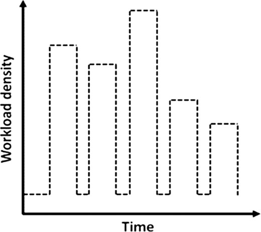
On-off workload pattern.
In these types of workload scenarios, terminating most of the running containers at once when the number of requests instantly decreases a lot is not an appropriate adaptation action because more container instances running into the pool of resources will be necessary very soon. This non-conservative strategy may result in too many container terminations and instantiations with the consequent QoS degradation. In other words, the shutdown and start-up times of containers should be taken into account during on/off workload scenarios.
5. RESULTS
In our empirical evaluation, the httperf14 tool has been used to develop a load generator in order to produce various workload patterns for different analyses. To this end, five different workload scenarios have been inspected, as shown in Fig. 8.
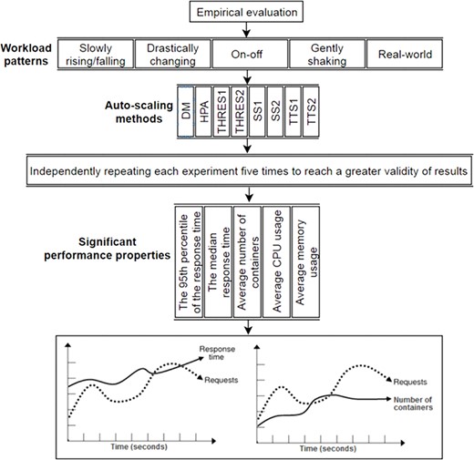
Experiment design to compare the new DM method to existing auto-scaling methods.
Each workload pattern examined in this work represents different type of applications. A slowly rising/falling pattern may imply incoming task requests sent to an e-learning system in which daytime includes more traffic than at night. A drastically changing pattern may represent a heavy workload to be processed by a broadcasting news channel in which a video or some news suddenly spreads in the social media world. This type of system generally has a short active period, after which the service can be provided at the lowest service level. Applications such as batch processing systems accomplish workload scenarios similar to the on-off workload pattern in which requests tend to be accumulated around batch runs regularly over short periods of time. A gently shaking pattern indicates predictable environments such as household settings that allow application providers to specify detailed requirements, and then allocate the exact amount of resources to the system.
Our proposed method called the ‘DM’ auto-scaling approach has been compared with different rule-based provisioning policies explained in Section 2.2. These approaches include HPA (Horizontal Pod Auto-scaling), TTS1 (Target Tracking Scaling—first method), TTS2 (Target Tracking Scaling—second method), SS1 (Step Scaling—first method), SS2 (Step Scaling—second method), THRES1 (THRESHOLD—first method) and THRES2 (THRESHOLD—second method). We kept the implementation of all these auto-scaling approaches and experimental data available at GitHub [41]. However, we did not implement MP, as this provisioning policy is not revealed clearly in terms of technical feasibility by Google Cloud Platform.
Each experiment has been repeated for five iterations to find the average values of significant properties and to verify the achieved results and hence to reach a greater validity of results. Therefore, the reported results are mean values over five runs for each experiment.
In every experiment, each auto-scaling method has been investigated primarily based on the 95th percentile of the response time, the median response time, average number of containers, average CPU usage and average memory usage.
Since the workload trends examined in our experiments are considered neither even nor predictable, the thresholds TCPU and Tmem are set to 80%. Hence, the DM method will have enough chance to react to runtime variations in the workload because these thresholds are not very close to 100%. This fact will also prevent an over-provisioning problem because these thresholds are not less than 80%. The constant α is set to the value of 5 which can prevent not only too frequent changes in the number of running container instances, but also too much over-provisioning of resources according to the rationale explained in Section 4.4.
A finite element analysis application useful for solving engineering and mathematical physics problems has been developed and containerized to be used in this work as a use case [1]. In our use case, a single job usually takes 180 ms with our experimental setup in situations where the system is not overloaded. For the DM method, in order to avoid performance drop, the response time threshold () has been set to 190 ms that is neither very close to the value of usual time to process a single job (180 ms) nor much bigger than this value. Therefore, the DM auto-scaling method will be responsive to changes in not only infrastructure utilization, but also application response time because is not much bigger than the usual time to process a single job.
When it comes to response time guarantees, determining the difference between auto-scaling methods in capability of providing response time under different workload patterns is considered informative. To this end, as shown in Table 4, DM was compared with all other methods using paired Student’s t-tests with respect to all response time values over the experimental period for each workload pattern (n = 145). The 95th percentile value of response time, shown in Table 5, is an indicator of the auto-scaling methods’ ability to deliver QoS according to a service level agreement (SLA). The median response time achieved by all investigated auto-scaling methods in every workload pattern is shown in Table 6.
P-values obtained by comparison of the DM method with other seven auto-scaling methods using paired t-tests with respect to all response time values over the experimental period for each workload pattern.
| Workload scenario | HPA | THRES1 | THRES2 | SS1 | SS2 | TTS1 | TTS2 |
|---|---|---|---|---|---|---|---|
| Slowly rising/falling | 0.18800 | 0.14650 | 0.75633 | 0.00568 | 0.00033 | 0.00118 | 0.00009 |
| Drastically changing | 0.00055 | 0.00000 | 0.00000 | 0.00385 | 0.00000 | 0.00000 | 0.00000 |
| On-off | 0.00000 | 0.00191 | 0.00115 | 0.00000 | 0.00000 | 0.00000 | 0.00000 |
| Gently shaking | 0.00032 | 0.15528 | 0.00004 | 0.00051 | 0.63366 | 0.00000 | 0.00000 |
| Real-world | 0.00014 | 0.00718 | 0.00001 | 0.00000 | 0.00005 | 0.00424 | 0.00000 |
The 95th percentile of the response time achieved by all investigated auto-scaling methods in every workload pattern.
| Workload scenario | HPA | THRES1 | THRES2 | SS1 | SS2 | TTS1 | TTS2 | DM |
|---|---|---|---|---|---|---|---|---|
| Slowly rising/falling | 213.07 | 202.40 | 208.21 | 364.70 | 372.90 | 365.20 | 398.90 | 207.40 |
| Drastically changing | 652.82 | 659.90 | 619.20 | 852.06 | 1623.14 | 1609.22 | 1270.98 | 410.28 |
| On-off | 471.75 | 386.00 | 387.90 | 683.70 | 493.60 | 550.40 | 566.50 | 232.60 |
| Gently shaking | 201.83 | 196.04 | 195.89 | 194.80 | 195.00 | 268.69 | 240.47 | 194.85 |
| Real-world | 204.64 | 208.84 | 214.26 | 202.94 | 233.64 | 215.66 | 260.2 | 197.32 |
The median response time achieved by all investigated auto-scaling methods in every workload pattern.
| Workload scenario | HPA | THRES1 | THRES2 | SS1 | SS2 | TTS1 | TTS2 | DM |
|---|---|---|---|---|---|---|---|---|
| Slowly rising/falling | 190.6 | 189.6 | 188.7 | 190.7 | 192.9 | 189.6 | 192.1 | 191.2 |
| Drastically changing | 185.6 | 193.0 | 199.1 | 190.5 | 197.9 | 199.4 | 201.0 | 190.1 |
| On-off | 199.6 | 191.3 | 195.5 | 194.5 | 200.7 | 209.7 | 211.4 | 190.5 |
| Gently shaking | 189.9 | 186.1 | 188.7 | 187.9 | 184.9 | 196.1 | 196.7 | 185.3 |
| Real-world | 193.4 | 192.0 | 194.4 | 195.3 | 193.9 | 195.3 | 197.4 | 192.3 |
Table 7 presents the resource utilization of all auto-scaling methods for all workload patterns in terms of average number of containers, average CPU usage and average memory usage. In this table, there is a column called resource utilization function which equals to the average number of containers multiplied by the 95th percentile of the response time achieved by auto-scaling methods for each workload pattern. It should be noted that in order to improve the resource utilization of an auto-scaling method while producing acceptable response time, the value of this function should be decreased as much as possible.
Comparing the new DM method with existing auto-scaling methods with respect to resource utilization.
| Workload scenario | Method | Resource utilization | Resource utilization function | ||
|---|---|---|---|---|---|
| Average number of containers | Average CPU usage | Average memory usage | |||
| Slowly rising/falling pattern | DM | 3.47 | 64.36 | 31.55 | 719.68 |
| HPA | 3.25 | 65.48 | 31.60 | 692.48 | |
| THRES1 | 3.65 | 62.24 | 31.50 | 738.76 | |
| THRES2 | 3.52 | 64.84 | 31.64 | 732.90 | |
| SS1 | 4.36 | 55.85 | 31.57 | 1590.09 | |
| SS2 | 3.84 | 61.86 | 31.73 | 1431.94 | |
| TTS1 | 3.12 | 71.85 | 31.56 | 1139.42 | |
| TTS2 | 3.32 | 70.78 | 31.58 | 1324.35 | |
| Drastically changing pattern | DM | 3.71 | 41.07 | 31.69 | 1522.14 |
| HPA | 2.50 | 50.77 | 31.68 | 1632.05 | |
| THRES1 | 3.31 | 40.72 | 31.58 | 2184.27 | |
| THRES2 | 3.31 | 40.92 | 31.51 | 2049.55 | |
| SS1 | 3.53 | 41.54 | 31.43 | 3007.77 | |
| SS2 | 2.47 | 45.22 | 31.68 | 4009.15 | |
| TTS1 | 2.68 | 45.69 | 31.63 | 4312.71 | |
| TTS2 | 2.68 | 45.84 | 31.71 | 3406.23 | |
| On-off pattern | DM | 3.58 | 53.49 | 31.40 | 832.71 |
| HPA | 2.77 | 66.90 | 31.50 | 1306.75 | |
| THRES1 | 3.39 | 57.25 | 31.55 | 1308.54 | |
| THRES2 | 3.40 | 58.27 | 31.74 | 1318.86 | |
| SS1 | 3.23 | 51.50 | 31.61 | 2208.35 | |
| SS2 | 2.71 | 58.53 | 31.72 | 1337.66 | |
| TTS1 | 2.33 | 64.90 | 31.69 | 1282.43 | |
| TTS2 | 2.33 | 64.65 | 31.70 | 1319.94 | |
| Gently shaking pattern | DM | 4.00 | 66.67 | 31.75 | 779.40 |
| HPA | 3.78 | 70.46 | 31.80 | 762.92 | |
| THRES1 | 4.00 | 66.94 | 31.58 | 784.16 | |
| THRES2 | 3.68 | 72.10 | 31.61 | 720.87 | |
| SS1 | 4.25 | 64.31 | 31.49 | 827.90 | |
| SS2 | 4.00 | 67.74 | 31.76 | 780.00 | |
| TTS1 | 3.41 | 79.25 | 31.62 | 916.23 | |
| TTS2 | 3.38 | 78.95 | 31.63 | 812.79 | |
| Real-world pattern | DM | 10.15 | 72.38 | 31.59 | 2002.80 |
| HPA | 9.20 | 75.81 | 31.55 | 1882.69 | |
| THRES1 | 9.86 | 71.02 | 31.61 | 2059.16 | |
| THRES2 | 9.98 | 70.32 | 31.56 | 2138.31 | |
| SS1 | 10.16 | 73.15 | 31.60 | 2061.87 | |
| SS2 | 9.38 | 74.23 | 31.59 | 2191.54 | |
| TTS1 | 7.27 | 79.09 | 31.60 | 1567.85 | |
| TTS2 | 7.64 | 75.44 | 31.62 | 1987.92 | |
Our experiments show that the period of time taken to start up a container instance is almost 6 s. In the experiments, the adaptation interval, which is the time period between two possible successive adaptation events (increasing or decreasing the number of cluster nodes), was defined as 30 s to make sure there would be no problem if any auto-scaling action occurs. While the monitoring interval can be specified as very short in milliseconds, it is set to 30 s to reduce the communication traffic load and any monitoring overhead for the measurements.
Table 8 shows the features of all machines used in our experiments. All these machines belong to a non-profit cloud-based infrastructure provider called ARNES (the Academic and Research Network of Slovenia). In our experiments, all host machines allocated to the cluster which provides the finite element analysis application have the same hardware features. Twelve hosts have been used in the cluster during the experiments.
Features of infrastructures used in our experiments.
| Feature | Load-Balancer | Monitoring Server | Hosts in the cluster |
|---|---|---|---|
| OS | Ubuntu 14.04 | Ubuntu 14.04 | Ubuntu 14.04 |
| CPU(s) | 4 | 2 | 4 |
| CPU MHz | 2397 | 2397 | 3100 |
| Memory | 16 384 MB | 4096 MB | 4096 MB |
| Speed | 1000 Mbps | 1000 Mbps | 1000 Mbps |
| Feature | Load-Balancer | Monitoring Server | Hosts in the cluster |
|---|---|---|---|
| OS | Ubuntu 14.04 | Ubuntu 14.04 | Ubuntu 14.04 |
| CPU(s) | 4 | 2 | 4 |
| CPU MHz | 2397 | 2397 | 3100 |
| Memory | 16 384 MB | 4096 MB | 4096 MB |
| Speed | 1000 Mbps | 1000 Mbps | 1000 Mbps |
5.1. Slowly rising/falling workload pattern
In this scenario as shown in Fig. 9, the workload includes two steps. In the first step of the workload scenario, the number of incoming requests slowly rises from 100 to 1500 requests per 6 s. Afterwards, during the second step, workload density drops smoothly from 1500 to 100 requests. Figure 9 shows that the number of containers increases in the first step of the workload scenario, and it decreases in the second step according to the number of arrived requests at execution time by all eight provisioning methods.
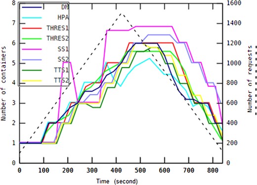
Dynamically changing number of container instances in response to a slowly rising/falling workload pattern.
For the slowly rising/falling workload pattern, the paired t-tests comparing DM with HPA, THRES1 and THRES2 reveal no statistically significant difference with P > 0.01. While all auto-scaling approaches are able to provide acceptable performance on average, the response time offered by SS1, SS2, TTS1 and TTS2 is sometimes lowin comparison to DM, HPA, THRES1 and THRES2. This is because the adaptation interval used in SS1, SS2, TTS1 and TTS2 is 1 minute versus 30 s used in DM, HPA, THRES1 and THRES2. Hence, the response time can be inappropriate for a while in some situations if the adaptation interval is not short enough, as shown in Fig. 10. This fact resulted in relatively weaker performance of SS1, SS2, TTS1 and TTS2 compared to DM, HPA, THRES1 and THRES2 with regard to the 95th percentile values.
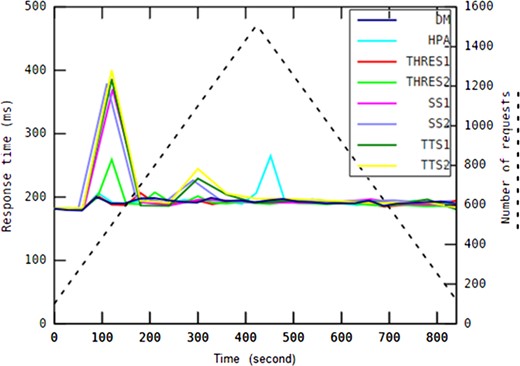
Average response time of the application in response to a slowly rising/falling workload pattern.
The length of the adaptation interval, whether 30 s or 1 minute, used by auto-scaling methods affects the overall application performance. For example when t = 90 s and before the CPU run queue would start filling up (~96%), DM decided to allocate one new container because of the increase in the workload. Therefore, the response time offered by DM was not affected by the workload increase. Considering another auto-scaling method called SS1, in such situation when t = 120 s and after the system was overloaded as a consequence of the growing workload, SS1 added four new containers to the cluster. However, at this time the processor utilization already reached almost 100%, and hence the slow response time was provided by SS1 for a while. Now the cluster includes five container instances. This cluster size is more than what is needed to handle the current workload. Therefore, this decision is reverted after a while when t = 240 s, and two container instances are terminated.
It should be noted that DM, HPA, THRES1 and THRES2 use almost the same number of container instances and have almost the same level of average resource utilization in terms of CPU and memory usage for the slowly rising/falling workload pattern. The SS1 provisioning approach allocated more container instances (4.36) compared to all other adaptation policies.
Moreover, the authors simply concluded that the finite element analysis application is not memory-intensive, as the average memory usage was almost steady during the conducted experiment, and the same for all auto-scaling approaches—around ~31% of the whole memory.
5.2. Drastically changing workload pattern
Here, drastic fluctuations appear in the workload intensity. In this experiment, shown in Fig. 11, the number of arrival requests changes suddenly from 100 to 1500, and after a while it instantly comes back to 100 requests again. For this workload pattern, the paired t-tests implied that there is a statistically significant difference between DM and all other auto-scaling methods. Figure 11 shows that our proposed method (DM) properly recognized the sudden increase in the workload and then tried to timely initiate enough container instances at the beginning of unexpected workload surge faster than other auto-scaling approaches. Therefore, for the drastically changing workload pattern, DM is the only method able to provide relatively convenient performance in terms of the 95th percentile of the response time distribution.
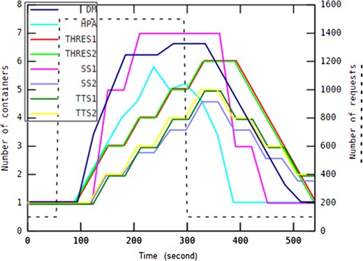
Dynamically changing number of container instances in response to a drastically changing workload pattern.
After a while, when the workload immediately drops again to 100 requests per 6 s, all auto-scaling approaches, except HPA and SS1, do not stop container instances running in the cluster at once, and consequently the number of containers slightly decreases in successive intervals. The method which provisioned more container instances than other auto-scaling approaches was DM. The average number of containers allocated by DM during this experiment was 3.71.
Figure 12 shows that the response time provided by DM, compared to other approaches, is less inappropriately impacted by the drastic change in the workload density.
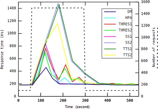
Average response time of the application in response to a drastically changing workload pattern.
Again, the amount of average memory usage was nearly constant (~31% of the memory capacity), and the same for all auto-scaling approaches during the whole conducted experiment in this workload scenario, considered as further confirmation of a slowly rising/falling workload scenario’s result, implying that the conducted application is not a memory-intensive benchmark.
5.3. On-off workload pattern
In this experiment, the on-off workload pattern has three active periods. The active periods include, respectively, 1500, 1200 and 700 requests per 6 s (shown in Fig. 13). Inactive periods between peak spikes are 30 s. For the on-off workload pattern, the paired t-tests showed a statistically significant difference in the means of response time metric offered by all auto-scaling methods. The only method able to timely provision an appropriate number of container instances in response to peak spikes is DM. Because it is more agile than other auto-scaling approaches in order to initiate necessary container instances at the beginning of unexpected workload surges, and also it does not terminate most of the containers immediately when each peak spike disappears. Consequently, DM has allocated more container instances on average (3.58) than other approaches during the on-off workload pattern.
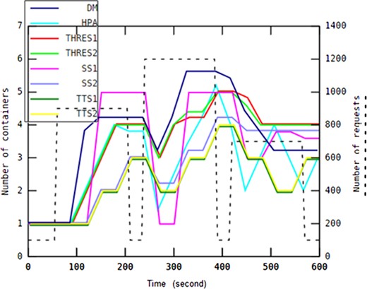
Dynamically changing number of container instances in response to an on-off workload pattern.
The advantage of using 30-s adaptation interval instead of one-minute interval can be understood in Fig. 13. At the beginning of the first active period, DM and SS1 took similar decision to increase the number of containers because of the sudden increase in the workload. DM allocated three extra containers starting from t = 90 s whereas SS1 allocated four new containers when the system is already overloaded at t = 120 s, or in other words 30 s later than t = 90 s. In such situation, the competence of DM compared to SS1 exists in its agility to timely adapt the application performance to the sudden increase in the workload. As a consequence, in this workload scenario the difference between DM and SS1 in terms of response time can be considered enormous. That is why the worst response times provided by DM and SS1 during the first active period were 225.04 ms versus 558.88 ms, respectively.
For the on-off workload pattern, the median and the 95th percentile of the response time provided by DM in this experiment were 191.2 and 232.60 ms, respectively, that can be considered acceptable with regard to users’ satisfaction. Whereas sudden active periods inappropriately cause an increase in the service time of the requests for the other seven auto-scaling methods, as shown in Fig. 14. Compared to the DM method, the 95th percentile values of the response time achieved by all other auto-scaling methods are very slow that can be considered inappropriate.
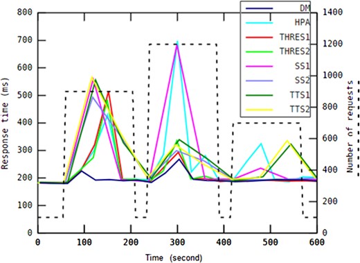
Average response time of the application in response to an on-off workload pattern.
In this experiment, the average memory usage was found to be consistent (~31%) for all auto-scaling methods, and it did not vary with the increase in the number of requests at runtime.
5.4. Gently shaking workload pattern
In this scenario, there exists a trembling workload which does not change drastically. As shown in Fig. 15, it frequently varies between 700 and 1000 requests to be processed by the application. Figure 15 indicates that if the workload does not change drastically, there is neither increment nor decrement in the number of running containers for DM, THRES1 and SS2. This is why, for this workload pattern, the paired t-tests comparing DM with THRES1 and SS2 showed that we cannot reject the zero hypothesis (P > 0.01), essentially meaning that the DM method behaves the same way as the THRES1 and SS2 methods. The number of containers has also not been changed to a great extent by other approaches namely HPA, THRES2, SS1, TTS1, and TTS2.
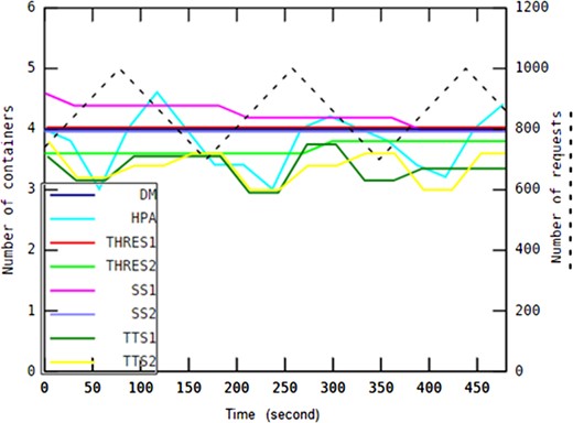
Dynamically changing number of container instances in response to a gently shaking workload pattern.
The SS1 auto-scaling policy allocated more container instances on average (4.25) than other approaches, whereas the average response time provided by all provisioning approaches (shown in Fig. 16) was nearly steady and identical for this workload scenario.
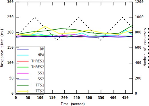
Average response time of the application in response to a gently shaking workload pattern.
Therefore, allocating more container instances by SS1 in this workload scenario undesirably caused resource under-utilization, in terms of less average CPU resource utilization, and reported 64.31% in comparison to what was achieved by other methods. However, all auto-scaling approaches achieved approximately the same level of memory usage (~31%) during the experiment.
5.5. Real-world workload pattern
In addition to the previous workload patterns, in order to validate the applicability of our proposed approach against real-world situations, FIFA World Cup 98 workload dataset [42] has been also applied in this work. This workload trace has been widely used in different auto-scaling research works [7, 43–47] so far. For our experiment, we used a 20-minute trace (shown in Fig. 17) on the 12 July 1998 starting at 20:30:00. The number of incoming requests per 6 s is varied between 2112 and 2858 during this time period that represents a large variance (~750) in the workload density at runtime.
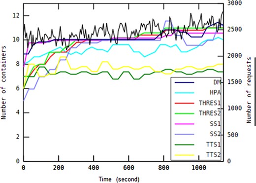
Dynamically changing number of container instances in response to a real-world workload pattern.
To adapt the application to the changing workload and achieve a desired performance, the number of running container instances allocated by auto-scaling methods varies over time. DM and SS1 provisioned the same amount of resources in terms of container instances on average for the real-world workload pattern. For both methods, the average number of containers was equal to 10.1. Other methods allocated fewer container instances compared to DM and SS1 in this experiment.
Figure 18 shows the average response time provided by all investigated auto-scaling methods in response to this real-world workload pattern.
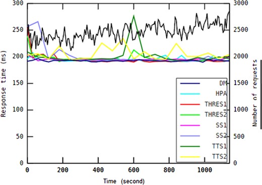
Average response time of the application in response to a real-world workload pattern.
For the real-world workload pattern, the response time offered by DM was not affected by the workload variations, since it was quite steady in comparison to what was provided by other approaches. In other words, there is no big difference between the 95th percentile of the response time distribution (197.32 ms) and the median response time (192.3 ms) obtained by DM.
Similar to the result concluded in previous workload patterns, the experiment in this scenario also re-implies that the memory resource utilization of the cluster does not have any influence on the performance of the finite element analysis application regardless of the number of incoming requests, because, it was ~31% for all auto-scaling methods during execution. This fact fortunately helps the cloud-based service provider to achieve efficient memory allocation for running container instances in advance.
For each auto-scaling method, all values of resource utilization functions achieved in every workload pattern were summed together to form an overall score. The scores are DM = 5856.73, HPA = 6276.89, THRES1 = 7074.89, THRES2 = 6960.49, SS1 = 9695.98, SS2 = 9750.29, TTS1 = 9218.65 and TTS2 = 8851.23. These results show that the DM auto-scaling method is the best among eight investigated approaches. This is because our proposed DM auto-scaling approach achieved the minimum overall score in comparison to the other approaches. It means that it is able to avoid over-provisioning of resources while offering optimal application performance in terms of the response time. Considering all workload scenarios examined in this work, the strength of the DM method lies in its ability to apply a multi-level monitoring framework and timely adjust itself to changes in the workload density over time.
The cumulative distribution function (CDF) of response time observed by all auto-scaling methods is shown from Fig. 19 to Fig. 23 for each workload pattern. It can be concluded that DM performs better than other methods as it has higher probability to offer desired response time under varied amount of workloads, and hence improve the application QoS. The probability that the response time provided by DM would be slow is approximately zero for all workload scenarios, except for the drastically changing pattern. Figure 20 shows that the response time provided by DM was relatively more appropriate than other seven auto-scaling methods during the drastically changing workload. In this workload scenario, the probability of response time being fast provided by other methods is significantly small.
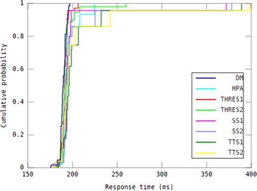
CDF of response time observed for the slowly rising/falling workload pattern.
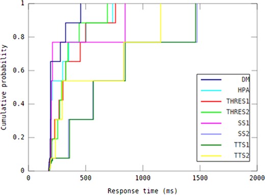
CDF of response time observed for the drastically changing workload pattern.
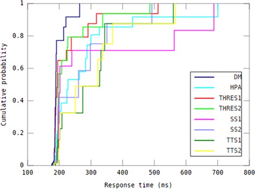
CDF of response time observed for the on-off workload pattern.
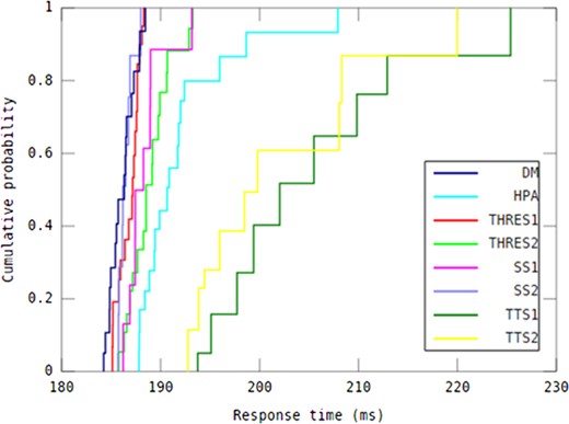
CDF of response time observed for the gently shaking workload pattern.
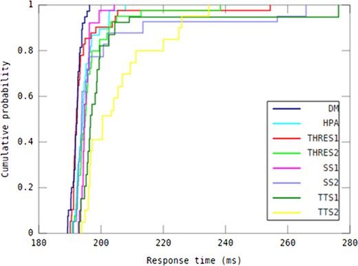
CDF of response time observed for the real-world workload pattern.
6. DISCUSSION
The obtained results allow analysis of the developed auto-scaling method and its limitations, its usability in the software engineering domain, comparisons with other rule-based methods, and the level of improvement in the effectiveness of self-adaptation for handling different workload scenarios.
An important part which has been investigated is the monitoring interval. Setting up an appropriate monitoring interval is required to ensure the reliability of the whole system, to avoid overhead, and to prevent losing control over the running environment during auto-scaling actions [48]. Defining an effective measurement interval is a challenging task, because a low level of measurement ratio may lead to missing dynamic changes of operational environments, and hence the system is not capable of adapting to a new situation to continue its operation without any performance issue.
In some cases, the difference between the monitoring interval and the average response time of the application may cause stability issues to the elasticity mechanism, which is not the case for many applications such as finite element analysis. For example, within video conferencing systems, violations of QoS constraints need to be monitored carefully, since even a small amount of violation should not be disregarded. Therefore, the monitoring interval should be short enough to adequately capture all necessary characteristics of the application over time. Moreover, self-adaptation of such applications also requires a high level of agility, which has recently gained a wide range of attention as a research field that still needs to be fully improved.
The proposed method can be extended to also consider vertical scaling of containers [49]. Vertical scaling is an option to resize processing power, memory capacity, or bandwidth assigned to container instances depending on runtime workload variations. However, the maximum amount of resources such as CPU or memory available for each container is limited to the host machine capacity. Therefore, the combination of vertical and horizontal scaling techniques can be applied to the same application in order to take advantages of both mechanisms. However, it should be noted that some applications such as Java/J2EE solutions [50] are not able to dynamically manage the memory allocation even if the memory capacity can be resized at the infrastructure or operating system (OS) level. In such cases, the applications have to be restarted with new resized memory when vertical scaling occurs.
The experiments in this work are based on Docker technology, however the proposed auto-scaling architecture can be implemented in other containerization technologies such as OpenVZ,15 LXC16 and lmctfy.17 This is because all functions defined in both Alarm-Trigger and Self-Adapter, as well as the StatsD protocol used to send, collect, and aggregate monitoring statistics related to any application or infrastructure, are independent from not only container virtualization technologies, but also underlying cloud infrastructure providers.
The implemented multi-level monitoring system of the SWITCH platform used in this work is capable of monitoring different container-level metrics namely CPU, memory, bandwidth, and disk [2]. This monitoring system has been employed to measure bandwidth and disk for a containerized file upload use case in our previous work [51].
Over the entire course of experimentation, different threats to the validity of the results have been analysed as follows:
Variations in runtime conditions (e.g. time-varying processing delays, I/O and CPU load factors, etc.) may slightly affect the results shown in Table 5. In order to reach a greater validity of results, each experiment on each workload pattern was repeated five times to avoid this threat. Therefore, the reported results are presented as average values over independent runs.
Cloud infrastructure QoS properties, e.g. availability, bandwidth quality etc. may vary over time, independently of the workload features. Therefore, when a container has to be deployed on a host machine, the application provider needs to make sure that the host is able to fulfil the requirements of the containerized application. To this end, the performance of infrastructures should also be continuously characterized. This is currently facilitated by the employed multi-level monitoring system of the SWITCH platform.
Various additional external factors (e.g. end-users’ network channel diversity, unstable network conditions at the client’s side and the mobility of the clients) may affect the users’ experience. In reality, cloud-based services are being used by different end-users from all over the world. This type of quality problems due to connectivity issues are currently being addressed by edge computing approaches [2].
Proposing a container-based auto-scaling method without relying on over-provisioning of resources is an important challenge in the adaptation of cloud-based applications. The principle which allows host machines to include one container instance per application type (e.g. CPU, memory, or bandwidth intensive), explained in Section 3.3, may cause over-provisioning among some clusters when there are applications which experience a small number of incoming requests. To come up with a solution to solve this limitation, in addition to the containers, host machines can be also adjusted vertically at runtime [52]. Another solution can be using different host machines in terms of hardware features allocated for each cluster according to the application types. For example, hardware characteristics of nodes which host a CPU-intensive application can be different from configurations of nodes which host a memory-intensive application. The former needs host machines with sufficient CPU, and the later requires host machines with enough memory.
7. CONCLUSION
Fine-grained auto-scaling mechanisms are needed to cope with highly dynamic workloads in the cloud environment. Existing traditional application adaptation approaches using a set of fixed rules unfortunately cannot accurately provide favourable service quality while offering optimal resource utilization. This paper introduced a new DM auto-scaling method which applies dynamic rules to automatically increase or decrease the total number of computing instances in order to accommodate varied workloads.
The proposed adaptation method innovatively uses a multi-level monitoring system since the adaption of containerized applications should be tuned and handled at various levels of cloud environments—container level and application level. The conducted experiments have demonstrated the benefits of our approach which can be considered the best among eight investigated auto-scaling methods. Particular benefits of using the proposed DM method are that it avoids under-provisioning as well as over-provisioning of resources, while it prevents QoS degradation and cost overruns at execution time.
We have begun extending our proposed method towards a multi-instance architecture and high level of service customization [53]. This architecture applies one application instance per one user or one type of users. It means there are different application instances for different users with various needs. In this model, any self-adaptation mechanism would need to consider more sophisticated options, such as setting up a new monitoring environment for a different type of application instance, which will add to the complexity of the adaptation process for the application.
ACKNOWLEDGEMENTS
The authors are thankful to the Academic and Research Network of Slovenia (ARNES) for use of their public cloud infrastructure.
FUNDING
This project has received funding from the European Union’s Horizon 2020 Research and Innovation Programme under grant agreement No. 643963 (SWITCH project: Software Workbench for Interactive, Time Critical and Highly self-adaptive cloud applications). and grant agreement No. 732339 (PrEstoCloud: Proactive Cloud Resources Management at the Edge for Efficient Real-Time Big Data Processing).
Footnotes
Docker, https://www.docker.com/
CoreOS, https://coreos.com/
Microsoft Azure, https://azure.microsoft.com/
Amazon EC2, https://aws.amazon.com/ec2
Kubernetes, https://kubernetes.io/
OpenShift Origin, https://www.openshift.org/
cAdvisor, https://github.com/google/cadvisor
Grafana, http://grafana.org/
Prometheues, https://prometheus.io/
Scout, https://scoutapp.com/
The SWITCH project, http://www.switchproject.eu/
The StatsD protocol, https://github.com/etsy/statsd/wiki
OpenVZ Linux Containers, http://openvz.org
lmctfy, https://github.com/google/lmctfy
REFERENCES
Kubernetes Horizontal Pod Auto-scaling, https://kubernetes.io/docs/tasks/run-application/horizontal-pod-autoscale/. [Online; accessed March 10, 2018].
Amazon Target Tracking Scaling, http://docs.aws.amazon.com/autoscaling/latest/userguide/as-scaling-target-tracking.html. [Online; accessed March 10, 2018].
Amazon Step Scaling, https://aws.amazon.com/blogs/aws/auto-scaling-update-new-scaling-policies-for-more-responsive-scaling/. [Online; accessed March 10, 2018].
Google Multiple Policies Scaling, https://cloud.google.com/compute/docs/autoscaler/multiple-policies. [Online; accessed March 10, 2018].
The SWITCH Monitoring Server container image, https://hub.docker.com/r/salmant/ul_monitoring_server_container_image/. [Online; accessed March 10, 2018].
The SWITCH monitoring system, https://github.com/salmant/ASAP/tree/master/SWITCH-Monitoring-System. [Online; accessed March 10, 2018].
The SWITCH Alarm-Trigger component, https://github.com/salmant/ASAP/tree/master/SWITCH-Alarm-Trigger. [Online; accessed March 10, 2018].
The SWITCH Self-Adapter component, https://github.com/salmant/ASAP/tree/master/SWITCH-Self-Adapter. [Online; accessed March 10, 2018].
