


Abstract
The correspondence of active learning and testing of finite-state machines (FSMs) has been known for a while; however, it was not utilized in the learning. We propose a new framework called the observation tree approach that allows one to use the testing theory to improve the performance of active learning. The improvement is demonstrated on three novel learning algorithms that implement the observation tree approach. They outperform the standard learning algorithms, such as the L* algorithm, in the setting where a minimally adequate teacher provides counterexamples. Moreover, they can also significantly reduce the dependency on the teacher using the assumption of extra states that is well-established in the testing of FSMs. This is immensely helpful as a teacher does not have to be available if one learns a model of a black box, such as a system only accessible via a network.
1. Introduction
Finite-state machines (FSMs) can model a wide variety of systems, such as communication protocols, hardware components or software projects. If a model of a system is not available explicitly or one wants to determine how the system behaves, machine learning methods can be used.
Knowing the inner representation of a system is the main goal of reverse engineering and it is a crucial part of many other related fields, for example, testing and verification. There are two main approaches to learning, active and passive. Passive learning derives a model of a system from given traces, or input sequences with corresponding responses. In contrast, active learning interacts with the system by asking for responses on particular input sequences chosen by the learner. The process of learning is stepwise, on each step a tentative model is expanded based on the output from a previous sequence and a sequence to query next is generated.
The contribution of the paper is to show the beneficial use of testing theory in active learning of FSMs. A new approach to learning will be described in Section 4. The improvement of the new approach emerges from the comparison with the framework that covers the standard learning algorithms such as the L* algorithm. Section 4 also proposes three new learning algorithms that are based on the new approach. The experimental evaluation in Section 5 then confirms the improvement in the learning by the new learning algorithms compared to the standard ones.
2. Background
This section defines the type of FSMs used in this paper and it explains testing and active learning on a simple example.
2.1. Finite-state machine
An FSM is a model consisting of states and transitions between states. According to the received input, the FSM changes its current state and responds with corresponding output. There are many different definitions of FSMs in the literature. Active automata learning deals with deterministic finite automata (DFA), whereas active learning of FSMs works rather with Mealy machines as they describe reactive systems more precisely. A Moore machine is another type of FSMs. The difference is mainly the position of outputs in a model. Moore machines and DFA have outputs tied to states. In contrast, outputs are only on transitions in the case of Mealy machines. This section proposes a general model called deterministic finite-state machine (DFSM) that have outputs both on states and on transitions.
There are two functions that describe the behavior of a model, a transition and an output functions. Generally, both functions take an input symbol and produce either a next state, that is, a state where the transition with the input leads, or an output symbol that is observed if the transition is followed. Two special symbols are introduced to cover both Moore and Mealy machines in one definition. An input symbol |$\uparrow $| called stOut requests the state output and the current state of the machine is not changed when asked. An output symbol |$\downarrow $| called noOut represents ‘no response’.
A DFSM is a septuple |$(S, X, Y, s_0, D, \delta , \lambda ) $|, where |$S $| is a finite nonempty set of states and |$s_0 $| is an initial state (|$s_0 \in S $|), |$X $| and |$Y $| are input and output alphabets (a finite nonempty sets of symbols, |$\uparrow \ \notin X $|), |$D $| is a domain of defined transitions; |$D \subseteq S \times X $|, |$D_\uparrow = D \cup \{S \times \{\uparrow \}\} $|, |$\delta $| is a transition function |$\delta : D_\uparrow \rightarrow S $| such that |$\forall s \in S: \delta (s, \uparrow ) = s $| and |$\lambda $| is an output function |$\lambda : D_\uparrow \rightarrow Y \cup \{\downarrow \} $|.
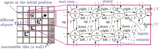
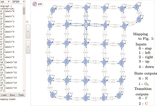
GridWorld map E and its part modeled by a DFSM.
Note that the stOut |$\uparrow $| is not in the input alphabet |$X $| so that it differs from all other input symbols. Similarly, the noOut |$\downarrow $| can be declared outside the output alphabet |$Y $| not to interfere with other output symbols but it is usually matched to the output of ‘timeout’ that is in |$Y $|. Therefore, it is not specified if |$\downarrow $| is or is not in |$Y $|. The timeout output represents the situation in which no response is observed during the predefined time limit. Strings over |$ X \cup \{\uparrow \} $| are called input sequences and strings over |$Y \cup \{\downarrow \} $| are called output sequences. ‘Input’ and ‘output’ are sometimes omitted so only ‘sequence’ is used if it is clear from the context. The empty string is denoted |$\varepsilon $|. An input sequence with the corresponding output sequence that was observed is called a trace. Any sequence |$w $| can be split into a prefix |$u $| and a suffix |$v $| where |$w = u \cdot v $|.
The initial state |$s_0 $| is the current state of the machine before any input is asked. Moreover, |$s_0 $| is also the current state if the machine is reset. Machines that can be reset are called resettable.
Transitions are labeled with input and output symbols. The next state, or the target state, of a transition is defined by the transition function |$\delta $| and the function |$\lambda $| assigns an output symbol to the transition. This paper works only with completely-specified machines, that is, DFSMs that have all transitions defined; |$D = S \times X $|.
An example of a DFSM is shown in Fig. 1. The model on the right captures a part of the map E shown on the left such that the map is formed of the grid of tiles and every tile is modeled by a state. The agent that is directed by the user can move in four directions and to explore the map. If the adjacent tile in a particular direction is not accessible, that is, it is outside the map or there is a wall, then the agent stays on the same tile and C is received as the response to the input corresponding to the direction. Otherwise, the agent moves in the chosen direction and the output F is obtained as the response. For instance, |$\delta (s_0, $| right|$) = s_2 $| and |$\lambda (s_0, $| right|$) = $|F. Each tile can contain an object. The agent asks the input |$\uparrow $| in order to find out which object is on the tile where the agent stands; there is usually nothing (the output N), for example, |$\lambda (s_0, \uparrow ) = $|N. Note that the agent does not move from the tile while exploring it, that is, |$\delta (s_i, \uparrow ) = s_i $| for any |$i $|. The map E (Fig. 1) is from the GridWorld scenario of the Brain Simulator [1]. The GridWorld scenario is similar to the toy environment that motivated the research of one of the first learning algorithm [2].
2.2. Testing of FSMs
A finite-state model of a system is very useful for construction of a test suite to test an implementation for equivalence to this model. There is a range of different testing methods known for this, originally developed for testing of communication protocols where testing is purely black box, that is, no internal structure of the implementation is known and it is not possible to observe a state such an implementation is in. A testing method would derive a series of tests from the model and if these sequences produce the same response from the model and the implementation, the implementation is deemed correct and otherwise faulty.
Derivation of test sequences requires an a priori knowledge of the upper bound on the number |$m $| of states in the implementation. Without such a bound, it is not practical to explore all of a state space and hence not possible to have any guarantee of equivalence by testing. Traditional DFSM testing methods (such as the W-method [3, 4]) generate test sequences to explore the state space of the model by visiting every state, attempting every input and then verifying entered states by observing how these states respond to sequences that distinguish them from other states in the model. The model, or the specification, is therefore assumed to be minimal. A machine is minimal if every state is reachable from the initial one and every two states |$s_i, s_j $| are distinguishable, that is, there is a sequence |$w $| that produces different output sequences when is asked from both |$s_i $| and |$s_j $|; |$w $| is called separating sequence of |$s_i, s_j $|. A set of separating sequences is called state characterizing set of |$s_i $| if for each state |$s_j $| different from |$s_i $| the set contains a separating sequence of |$s_i $| and |$s_j $|. In addition, state characterizing sets of all states are called harmonized state identifiers (HSI) if for each two states there is a common separating sequence in both corresponding sets.
An |$m $|-complete test suite is by definition one capable of finding all faults in an implementation of at most |$m $| states. Where a model has |$n<m $| states, one has to consider a possibility of redundant states in an implementation. These states also have to be tested in case they have different transitions leading from them compared to a model. Since it is not known how to enter these states, all sequences of inputs of length |$m-n $| have to be attempted in every state, followed by all possible inputs and then sequences to check the target state. This causes an exponential growth in the number of test sequences. More effective test methods generate sequences that do multiple things at the same time such as combine testing of transitions with checking of states entered by earlier transitions.
Active learning explained on the GridWorld example.
An example of separating and test sequences below is depicted using GridWorld map E in Fig. 1. A separating sequence of |$s_0 $| and |$s_7 $| is the stOut input |$\uparrow $| because there is an object on the tile corresponding to |$s_7 $|. The action ‘right’ separates |$s_9 $| from states |$s_0 $| or |$s_2 $|. If one wants to test the transition with input ‘down’ from |$s_6 $|, a test sequence consists of an access sequence of |$s_6 $| (‘right |$\cdot $| right’ for instance), then the transition ‘down’ and a separating sequence that identifies the target state |$s_7 $| (‘right |$\cdot $| left |$\cdot $||$\uparrow $|’); one of complete test sequences thus could be ‘right |$\cdot $| right |$\cdot $| down |$\cdot $| right |$\cdot $| left |$\cdot $||$\uparrow $|’. The choice of the separating sequence ‘right |$\cdot $| left |$\cdot $||$\uparrow $|’ is explained in Section 4 where so-called adaptive separating sequences are introduced.
2.3. Learning of FSMs
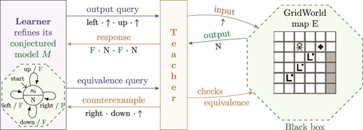
Active learning of FSMs usually consists of four entities as sketched in Fig. 2. There is a learner, a teacher, the black box and the conjectured model. The learner, or the learning algorithm, interacts with the black box through the teacher in order to construct the conjectured model |$M $| that is equivalent to the black box. There are two types of queries that the learner can ask. An output query (OQ), or a membership query in the case of automata learning, asks for the response to the given input sequence. This could be done without the teacher but in general, the teacher can operate as a mapper between symbolic and concrete inputs and outputs used by the learner and the black box. An equivalence query (EQ) is asked in order to check if the given conjectured model is output-equivalent to the black box, that is, if both machines respond equivalently to any input sequence. If they are not, a counterexample (CE) is provided to the learner.
For models of software, a ‘teacher’ is an unknown program. Therefore, EQ is usually approximated by testing where a testing method constructs test sequences based on the given conjectured model providing some confidence that both the conjectured model and the black box are equivalent. The amount of testing to confirm the correctness of a program is in the worst case exponential in the number of extra states (ESs). The example in Fig. 2 depicts the learner assuming that the GridWorld map E is modeled with the 1-state DFSM and so the CE to an EQ could be the sequence ‘right |$\cdot $| down |$\cdot \uparrow $|’.
3. Related Work
The field of active automata learning is based on the notion, proposed in [5], that each finite automaton is identifiable in the limit (from positive and negative examples). The L* algorithm was then proposed by Angluin in [6]. It learns using an observation table (OT) that stores observed responses in its cells and the labels of rows and columns form queries, that is, both rows and columns are labeled with input sequences. The rows can be separated into two parts. The first part represents observed states; labels of these rows are access sequences of states. The second part is labeled with one-symbol extensions of the access sequences, that is, it corresponds to next states. The L* algorithms aims to have an OT that is closed and consistent. An OT is closed if each row of the second part has the content equal to a row from the first part, that is, each transition leads to an observed state. An OT is consistent if for every two rows of the first part that are equal, the rows corresponding to their one-symbol extensions have the same content as well. In other words, if an observed state is accessed by different sequences, their extensions reach the same states (this is required because the machine is deterministic). When the OT is both closed and consistent, the OT defines an FSM |$M $| and so the algorithm asks an EQ that checks whether |$M $| correctly models the system. There are several versions of the algorithm that differ in processing of provided CEs. The original version by Angluin uses all prefixes of CE, thus here called L* – AllPrefixes. Other versions work with suffixes only, for example [2, 7, 8]. The best processing of long random CEs provides the version Suffix1by1 [9] that extends the set of separating sequences by suffixes of a CE (starting from the shortest) until the conjectured model responds to the CE correctly. L* was adjusted for Mealy machines in [10]. The discrimination tree (DT) algorithm [11] employs a classification tree to learn instead of an OT used by the L* algorithm. The DT algorithm was improved by the TTT algorithm proposed in [12].
A theoretic framework called observation pack (OP) for efficient active learning was set in [13]. The authors showed that the L* and DT algorithms implement their framework and provided lower bounds of numbers of output and EQs and their complexity. Moreover, they introduced a way to reduce the number of EQs by identifying all successors of states reached by a sequence of length up to the given number |$l $|. The OP algorithm proposed in the PhD thesis of Howar [14] combines a DT and OTs to infer Mealy machines. Its versions, OP—AllGlobally, OP—OneGlobally and OP—OneLocally, differ in the way how the distinguishing suffix of a CE is used. The thesis [14] also covers incremental approximation of EQs using a testing method. The GoodSplit algorithm [15] approximates EQs by querying random input sequences of limited length.
Correspondence of testing and active learning was studied, for example in [16] and [17]. A recent method, called here the quotient algorithm [18], inspired by testing of FSMs learns using the observation tree. It is based on one of the oldest testing methods, the W-method [3, 4]. There are more advanced testing methods such as the H-method [19], the SPY-method [20] or the SPYH-method [21]. An experimental evaluation of different testing methods of FSMs can be found in [22].
The most promising application of active learning and testing is adaptive model checking (AMC) [23] and gray box checking [24] that are based on black box checking [25]. Both AMC and gray box checking use testing as a task separated from the learning, hence, it duplicates a lot of queries that the learner already asked. AMC employs the L* algorithm to learn a model that is then passed to a model checker. If a discrepancy is found, it is checked against the system. A CE is returned to L* if the discrepancy is not confirmed in the system. On the other hand, if all properties hold in the conjectured model, the W-method is employed to test the model against the system. AMC thus provides software verification. The model checker is an additional oracle, which the work presented in this paper would also benefit from. Gray box checking uses knowledge about parts of the system that are so-called white boxes because the definition of their behavior is available as source code for example.
A framework is needed for experiments with learning approaches. Such tools are LearnLib [26], libalf [27] and FSMlib [22]. LearnLib is a JAVA framework with GUI for experimenting with learning process; libalf is a C++ library supporting remote execution and Java native interface. FSMlib is a new C++ library used in this paper for handling DFSM and it contains an implementation of numerous test generation and active inference methods [28].
4. Observation Tree Approach
The standard learning algorithms mentioned in the previous section have limitations addressed in this section by introducing a new framework called the observation tree approach. This approach allows one to use the testing theory in order to minimize the interaction with the black box and still learn its model.
This section is structured as follows. First, drawbacks of standard learning algorithms are discussed as they motivate the research of a new learning procedure. Then, the structure of an observation tree is defined and the new learning approach is proposed in Section 4.3. The learning using the approach is explained on an example in Section 4.4. Section 4.5 describes three new learners that implement the observation tree approach. A high-level description of dealing with inconsistencies is provided in Section 4.6. This section is concluded with a comparison against the OP framework and with the time complexity of the approach.
4.1. Motivation
The standard learning algorithms ask an EQ immediately after the conjectured model becomes completely-specified. Hence, the states of the black box are revealed mostly due to the provided CEs rather than a targeted exploration. This is captured best by the use of the DT algorithm that needs almost |$n $| EQs to learn a machine with |$n $| states. The L* algorithm does not need so many EQs but it requires many more OQs in order to learn a completely-specified model. The trade-off between the numbers of EQs and OQs was described by [13] based on the framework of an OP. The insufficient generality of the OP will be discussed at the end of this section after new learning algorithms are described.
There are two reasons to base active learning on methods of testing of FSMs:
a faster construction of a completely-specified conjectured model, and
a guided exploration of the black box based on the assumption of ESs.
The second reason to base active learning on testing is the assumption of ESs that allows the learner to provide the following guarantee.
(Complete learning guarantee). If the black box is different from the conjectured model of |$n $| states, then the black box has more than |$n+l $| states where |$l $| is the assumed number of ESs.
The guarantee relies on sufficient conditions that are formally proven for the described FSM testing methods. These conditions capture what should be observed in order to check the equivalence of two machines with bounded number of states. The conditions help learning algorithms to optimize which OQ to ask in order to reveal new states or gain the complete learning guarantee. Moreover, the number of asked EQs is decreased dramatically by the assumption of ESs. The experimental evaluation shows that the assumption of just one ES is sufficient to reveal most states and then there is no need for EQs that are hard to approximate for software.
4.2. Structure of an observation tree
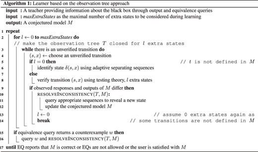
The observation tree approach is proposed in Algorithm 1. It provides a general framework for a learner to learn with the assumption of ESs based on the testing theory in order to reduce the number of EQs. All traces that are observed during learning are stored in the observation tree (OTree).
Given a set |$U $| of observed traces of a DFSM |$(S, X, Y, s_0, D, \delta , \lambda ) $|, the observation tree is a DFSM |$(R, X, Y, r_0, D_U, \delta _U, \lambda _U) $| such that for each trace |$u_i \in U $| there is a unique state |$r_i \in R $|, which only |$u_i $| leads to.
The observation tree basically groups observed traces with the same prefix. Its transition system has no cycles and looks like a tree with the root as the initial state |$r_0 $|. Hence, it corresponds to a prefix tree acceptor used in passive grammar inference, for example, by the Blue-Fringe algorithm [30]. The observation tree is the most suitable learning structure because it does not forget any observed trace in contrast with the classification tree of the DT algorithm and it stores each trace only once in contrast with the OT of the L* algorithm. In addition, the OTree corresponds to a testing tree that is used to capture test sequences while a testing method is constructing a test suite. Sequences of both the OTree and the testing tree consist of four parts: an access sequence, a tested transition, an extension and a separating sequence. Each state of the conjectured model (or of the specification in the case of testing) corresponds to a reference node (RN) of the OTree (or the testing tree) and each node is reached by a unique access sequence from the root of the OTree. Access sequences as the first parts of sequences in the OTree are used to lead to a particular state from which a transition is to be tested or the target state of the transition, which to be identified if it is not known. In contrast, separating sequences are used to identify the state in which they start. The third part, that is, the extension, is needed when one works with the assumption of ESs. These extensions have the length up to the considered number |$l $| of ESs in order to reach states that could be ‘extra’ with respect to the conjectured model, that is, such states could be different from those corresponding to the RNs. The purpose of the separating sequences is thus to determine if these states are different or not.
The correspondence between the conjectured model and the observation tree is based on the RNs that represent states of the conjectured model. Every two RNs are distinguished in the OTree by different responses to the same input sequence that starts in both RNs. Transitions are defined such that the target state is determined according to the corresponding successor |$r $| of the RN, that is, if there is a transition labeled with the input |$a $| leading from the RN of state |$s_i $| to the node |$r $| corresponding to the state |$s_j $|, then the conjectured model contains the transition |$(s_i, a) $| leading to |$s_j $|. The correspondence of the successor |$r $| and the state |$s_j $| is based on the sufficient conditions for the used FSM testing method that also depends on the number |$l $| of ESs. Basically, the successor |$r $| needs to be distinguished from the RNs of states different from |$s_j $| and the successors of |$r $| reached by a sequence of the length up to |$l $| need to correspond to a single RN as well. Moreover, these successors of |$r $| need to be distinguished one from the other if the one is a successor of the other one. If all the transitions are defined with respect to the assumed number |$l $| of ESs, then the observation tree is closed for |$l $| ESs.
4.3. Learning process
The learning process of the learner that is based on the OTree approach (Algorithm 1) can be divided into two phases. In the first phase, the learner constructs a completely-specified conjectured model as the standard learning algorithms do, that is, the observation tree is made closed for 0 ESs and all transitions are defined. In the second phase when the learner makes the OTree closed for the number |$l $| of ESs such that |$l> 0 $|, all transitions are considered defined but unverified. Note that undefined transitions are also unverified. Any response observed for the first time can break the consistency between the conjectured model and the OTree. It means that the conjectured model can no longer model the observed traces as the black box has more states than the conjectured model. The inconsistency is resolved by localizing a new RN that usually requires several OQs that distinguish a node from all current RNs. This process is described by the resolveInconsistency function (discussed later), which is also used after the teacher provides a CE in response to an EQ. The purpose of a CE is to show an inconsistency between the OTree and the conjectured model. After resolving the inconsistency, the transitions from the new state are usually not defined; therefore, the number |$l $| of assumed ES is reset to 0. If there is no inconsistency observed in the second phase and the number |$l $| reaches the given number maxExtraStates, an EQ can be asked. The learning can stop for three reasons: (i) either the conjectured model is correct as no CE is returned to an EQ, or (ii) EQs are not allowed at all because the teacher has no capability to answer this type of query, or (iii) the user is satisfied with the conjectured model. The last reason could be used in the following scenario. The user starts the learner with a large value for maxExtraStates. Most states are revealed by the assumption of 1 ES, that is, |$l = 1 $|. A few last states are harder to reveal and so the learner starts to increase |$l $|. The number of OQs grows exponentially with the increasing |$l $| and so it takes more time to reveal these ‘hidden’ states. The learner provides the user with the guarantee of |$l $| ESs (Definition 4.1) and the user can be satisfied with the number of revealed states so that the user stops the learning even if |$l $| does not reach the given maxExtraStates. The exponential growth is due to the complexity of FSM testing that nevertheless secures the guarantee.
The first phase of the learning depends on so-called adaptive separating sequences. An adaptive separating sequence groups separating sequences with the same prefix so that it looks like a tree. Each transition corresponds to an input and branches reflect different outputs from the black box. It is used to identify the target state of a transition that is not defined yet. If the corresponding node, that is, the successor of a RN, is not distinguished from more than one RN, then the separating sequences of these ‘undistinguished’ RNs captured in the OTree form adaptive separating sequences such that each starts with a different input symbol. To reduce the amount of testing, the input that distinguishes the most ‘undistinguished’ RNs is then queried. Note that only one separating sequence is queried out of all sequences that form the chosen adaptive separating sequence because the input to be queried next is selected based on the observed response to the previous input. This is a change compared to the standard learning algorithms that ask OQs on entire input sequences, not symbol by symbol. The use of adaptive separating sequences thus reduces the number of queried symbols.
Beginning of learning the GridWorld example.
4.4. Running example
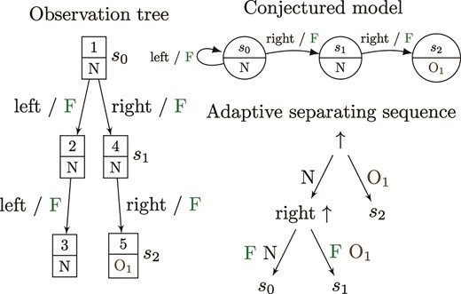
Figure 3 shows how the learning of the GridWorld map E (Fig. 1) could start. The observation tree on the left captures the first five queries that correspond to the numbers labeling nodes of the tree. At first, the output of the initial state is obtained by asking |$\uparrow $|. Then, the learner asks for the response on ‘left |$\cdot \uparrow $|’. The response N to |$\uparrow $| suggests that the transition on input ‘left’ leads back to the initial state |$s_0 $|. It is confirmed by the same response to ‘left |$\cdot \uparrow $|’ queried from the reached state |$\delta (s_0, $| left|$) $|. The fourth query checks the transition on ‘right’ from the initial state. The reached state produces the output N, hence, it seems to equal to |$s_0 $|. Nevertheless, the response to another ‘right |$\cdot \uparrow $|’ (fifth query) differs from the expected one. The observed difference leads to the identification of two states, |$s_1 $| and |$s_2 $|, that are reached by ‘right’ and ‘right |$\cdot $| right’ from the initial state, respectively. All three states can be distinguished by separating sequences ‘|$\uparrow $|’ and ‘right |$\cdot \uparrow $|’ that can be combined in the adaptive distinguishing sequence shown in Fig. 3.
4.5. Novel learners
The H-, SPY- and S- learners are novel learning algorithms that follow the observation tree approach and so outperform the standard learning algorithms. They differ in the choice of testing method by which they are inspired. It influences the choice of access and separating sequences as is summarized in Table 1. The H-learner is the simplest of the three. It is inspired by the H-method [19] and so it always uses the shortest access sequences of RNs. In the second phase of the learning, it chooses separating sequences on-the-fly from the observed ones in order to distinguish the reached node from one RN that corresponds to a different state. The SPY-learner is inspired by the SPY-method [20]. In addition to the shortest access sequences of RNs, it can employ the access sequence of nodes that were proven to be convergent with RNs. The convergence of two sequences (or the reached nodes of OTree) means that both sequences lead to the same state in all machines with up to |$m $| states that provide expected responses to queried sequences [20]. This paper considers the system to learn has at most |$m $| states where |$m $| equals the number |$n $| of states in the specification plus the number |$l $| of considered ESs. The convergence provides a way to minimize the number of OQs by appending the needed separating sequences over convergent sequences. The drawback of the SPY-learner is the use of fixed separating sequences formed in the HSI that is not so efficient compared to separating sequences chosen on-the-fly by the H-learner. The S-learner is similar to the SPY-learner in the first phase, that is, it utilizes the convergence of access sequences and employs adaptive separating sequences. The second phase is delegated to the S-method that is a new testing method that is an improvement of the SPYH-method [21]. It makes the given OTree (considered as a testing tree) closed for the given number of states by extending some sequences. It works with the convergence of sequences and separating sequences are chosen based on the splitting tree that allows one to distinguish most ‘undistinguished’ RNs. Hence, it is more efficient than the H- and SPY- methods. Their implementation can be found in the FSMlib [28].
The choice of access and separating sequences by the three new learners.
| Learner | Access sequences | Separating sequences |
|---|---|---|
| H-learner | Fixed | Chosen on-the-fly to distinguish from one RN |
| SPY-learner | Fixed + convergent | Fixed – formed in HSIs |
| S-learner | Fixed + convergent | Chosen on-the-fly to distinguish from most RNs |
| Learner | Access sequences | Separating sequences |
|---|---|---|
| H-learner | Fixed | Chosen on-the-fly to distinguish from one RN |
| SPY-learner | Fixed + convergent | Fixed – formed in HSIs |
| S-learner | Fixed + convergent | Chosen on-the-fly to distinguish from most RNs |
4.6. Resolving inconsistencies
An inconsistency of the conjectured model and the OTree can be observed in different ways depending on the implementation of the learner. All three new learners use the notion of domains of states associated with each node of the OTree. Domains capture the similarity of the corresponding node to the RNs. Hence, an RN |$s $| is not in the domain of node |$r $| if a separating sequence of |$s $| and |$r $| was observed. The basic inconsistency is revealed if a node |$r $| has an empty domain. It means that |$r $| is distinguished from all RNs and so it represents another state of the system; |$r $| becomes a new RN. Another type of inconsistency is when a node |$r $| should correspond to a particular state of the conjectured model but the corresponding RN |$s $| is not in the domain of |$r $|. Such an inconsistency is called inconsistent domain and can be resolved by querying several sequences that reveal the basic inconsistency in a form of an empty domain. The sequences are formed from the separating sequence of |$r $| and |$s $| (captured in the OTree) prepended with suffixes of the access sequence of |$r $|. The sequences are queried starting from the shortest and each is queried from the RN that corresponds to the node where the sequence begins in the OTree. There are two other types of inconsistency that can be observed by the SPY- and S- learners as they employ the convergence of sequences. Both learners group OTree nodes in convergent nodes (CNs) if their access sequences were proven to be convergent. It means that a so-called convergent graph is built on top of the OTree. If any two OTree nodes belonging to different CNs are shown to be convergent, then the CNs are merged so that the convergent graph is equivalent to the conjectured model in the end of learning. As all OTree nodes of a CN need to correspond to a single state, there are also CN domains that keep track which state the CN can correspond to. The inconsistency is observed if a CN domain is empty or if a CN cannot be merged successfully into the corresponding CN of RN because some of their successors are incompatible. These two inconsistencies are resolved by reducing the domain of a particular OTree node |$r $| using observed separating sequences of other OTree nodes that were (possibly incorrectly) in the same CN as |$r $|.
4.7. Comparison with an OP
The proposed observation tree approach is more general than the framework of OP [13] as the following shows. First, each state has a fixed verifying component of separating sequences in the OP; components thus correspond to HSIs. Therefore, the H-learner does not implement the OP framework. Second, the OP does not allow different access sequences of a single state, that is, the convergence of sequences is not considered. Therefore, the SPY- and S- learners do not implement the OP framework.
4.8. Time complexity
The time complexity of the observation tree approach depends mainly on the number of considered ESs. Any learner that uses a testing method to approximate EQs is bound by the time complexity of the used testing method. In the worst case, it is exponential in the number |$l $| of ESs with the base of the number |$p $| of inputs because all sequences of the length |$l $| need to be examined from every state in order to secure the guarantee (Definition 4.1). Nevertheless, the average case is nearly always much smaller. Theoretical evaluation of such an average complexity is the subject of future work. If no ES is considered, then the complexity relates to the size of the OTree, which is polynomial in the number |$n $| of states in this case. The complexity is also influenced by provided CEs that could be of arbitrary length in general.
5. Experiments
This section describes an experimental evaluation that aims to address the following two research questions:
Q1. Is practical complexity of automata inference using new methods significantly better than that of existing methods? Q2. Is it practical to learn accurate models in the presence of ESs?
The three new learners were compared with the standard learning algorithms experimentally on the GridWorld map E (Fig. 1), on three real system models and on a set of randomly-generated machines. GridWorld had no model available and so it was learnt by interaction and EQs were approximated by a testing method. The interaction with GridWorld was done through a mapper that translates symbolic inputs to real actions and observed responses to symbolic outputs. Hence, the GridWorld learning is the most realistic experiment. Random machines show that the learners are very effective on a range of different DFSMs and finally three models of real systems are shown where learners exhibit similar trends to both GridWorld and randomly-generated machines.
Learnt model of the GridWorld map E. States, inputs and outputs are numbered from 0. Highlighted state 0 (with the output 0 shown below) is the initial state.
5.1. GridWorld case study
The learnt model of the GridWorld map E is visualized in Fig. 4 using the FSMvis that is a part of the FSMlib. The learning metrics of six learners are captured in Table 2. The algorithms are compared on the numbers of resets, queried symbols, OQs, EQs, GridWorld simulation steps and the learning time in seconds. The three new learners were not allowed to ask EQ but they can learn the correct model with the assumption of only one ES. Therefore, when they assume two ESs, they also do not need the teacher but they provide a stronger guarantee about the states of the black box. The most efficient of the standard learning algorithms is the quotient algorithm that however needs four EQs (implemented by the SPY-method and 0 ES). Test sequences generated by the SPY-method are queried by the teacher starting with the shortest ones, hence, the shortest CE is provided. The results in Table 2 show the lowest number of ESs that the SPY-method needs to assume in order to find a CE for each faulty conjectured model that the standard learning algorithms create. A faulty conjectured model is simply each that has less than 32 states. It is not mentioned in Table 2 but the S-learner assuming 1 ES learns the map E only in 7894 simulation steps and in the next 23228 steps the learner verifies the absence of another state.
Learning GridWorld map E: learners are sorted by the number of simulation steps (last column) that corresponds to the amount of interaction, that is, the number of resets of the black box plus the number of symbols queried during the learning by both the learner and the teacher. The teacher gets a CE to EQs by the SPY-method.
| Learning algorithm | Resets | Symbols | OQs | EQs | Seconds | Steps |
|---|---|---|---|---|---|---|
| S-learner: 1 ES | 486 | 9784 | 3859 | 0 | 620 | 31122 |
| H-learner: 1 ES | 1026 | 10028 | 2618 | 0 | 829 | 41434 |
| Quotient | 1110 | 7487 | 1110 | 4 | 615 | 48652 |
| + SPY-method: 0 ES | 377 | 4835 | ||||
| SPY-learner: 1 ES | 1801 | 17415 | 4058 | 0 | 1345 | 74651 |
| S-learner: 2 ES | 2005 | 51300 | 20997 | 0 | 3443 | 156357 |
| H-learner: 2 ES | 4185 | 44325 | 10565 | 0 | 3314 | 186274 |
| TTT | 1363 | 7870 | 1363 | 11 | 4145 | 378793 |
| + SPY-method: 2 ES | 6864 | 131212 | ||||
| SPY-learner: 2 ES | 9630 | 96493 | 18177 | 0 | 8134 | 432450 |
| L*AllPrefixes | 3444 | 28062 | 3444 | 8 | 4664 | 445285 |
| + SPY-method: 2 ES | 5641 | 115749 |
5.2. Randomly generated machines
Figure 5 depicts the results of learning randomly-generated DFSMs. The algorithms were compared on 3400 DFSMs, 3400 Mealy machines, 3400 Moore machines and 3400 DFA such that all of them except DFA have five outputs. For each machine type, half of machines has 5 inputs and the others 10 inputs, both halves are divided into 17 groups of 100 machines with the same number of states that ranges from 10 to 1000. Target states of transitions and outputs are first chosen at random and then some are changed in order to create initially connected machine with the presence of each output symbol. If the generated machine is not strongly connected, then it is deleted and another machine is generated. A machine is strongly connected if there is a directed path between any two states. As the black box is known to the teacher, it provides the shortest CEs in response to an EQ if the conjectured model is not output-equivalent to the black box. The shortest CE is obtained by the breadth-first search in the product machine of the black box and the given conjectured model.
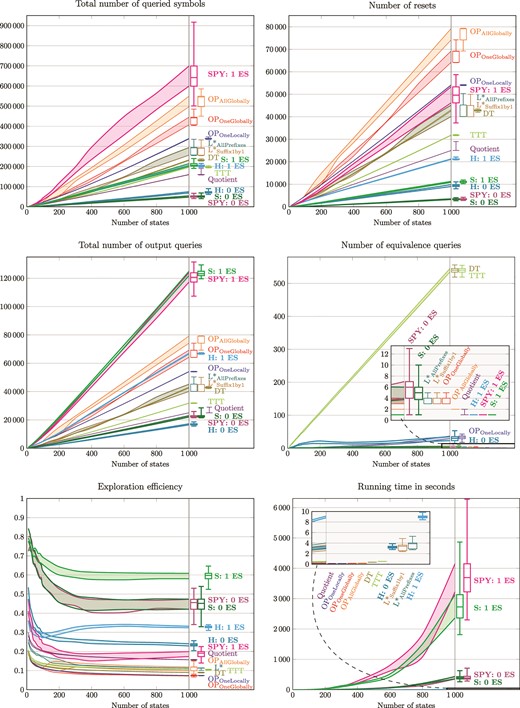
Comparison of learning algorithms on 17 groups of 100 randomly-generated DFSMs with 5 inputs and 5 outputs such that the groups vary in the number of states, from 10 to 1000.
The figures in Fig. 5 show the first and the third quartiles calculated for each ‘state group’ of 100 DFSMs with 5 inputs. In addition, the boxplots on the right of each graph also capture minimum and maximum values for the machines with 1000 states. All machines with the results are available in the GitHub repository FSMmodels [31].
The exploration efficiency (EE) is a new objective developed by the authors. It is calculated as the number of edges in the OTree divided by the total number of queried symbols. It permits one to evaluate how much of the black box is explored and how much effort was put in it. The greater the value, the better the learner is.
The new learners assuming 0 ESs can be directly compared with the standard learning algorithms. They outperform the DT and TTT algorithms in all measures (besides time). They are more efficient than the other standard algorithms in the numbers of OQs, queried symbols and resets and in the EE. However, they have a greater number of EQs because they build a completely-specified model fast with the least number of symbols, which means very little exploration and hence a low chance to find an inconsistency. This is balanced by the new learners assuming one ES that query about the same number of symbols as the standard algorithms but reset the black box less and need no EQ to learn. Moreover, they provide the guarantee at the end that there is not one ES. Note that all learners were allowed to ask EQ, therefore, they ask at least one EQ, the last one, which confirms that the conjectured model is correct. The DFSMs with 10 inputs as well as the 10200 randomly generated machines of the other three machine types produce results with the same trends of the learners’ performance as in Fig. 5.
5.3. Real systems
Table 3 shows the results of learning a scheduler. Its model is referred sched4 in the literature [12, 14] and it is a deterministic finite automaton with 97 states and 12 inputs. The teacher provides the shortest CEs. The results are similar for the other two models of real systems that are called peterson2 and sched5. The results also capture the same trends observed on randomly-generated machines (Fig. 5). Hence, the improvement by the new learners is more than promising. As in the case of randomly-generated machines, all three models with the results of experiments are available in the repository FSMmodels.
Learning sched4: learners are sorted by the amount of interaction, that is, the number of resets of the black box plus the number of input symbols queried during the learning.
| Learning algorithm | Resets | Symbols | EQs | Seconds | EE [%] |
|---|---|---|---|---|---|
| SPY-learner: 0 ES | 2007 | 25334 | 68 | 9.14 | 14.3 |
| S-learner: 0 ES | 2017 | 25438 | 65 | 9.09 | 14.0 |
| H-learner: 0 ES | 2307 | 28913 | 78 | 0.55 | 11.0 |
| TTT | 3606 | 43757 | 94 | 0.03 | 5.5 |
| DT | 11805 | 110183 | 96 | 0.05 | 2.2 |
| S-learner: 1 ES | 14107 | 178965 | 1 | 181.94 | 9.8 |
| H-learner: 1 ES | 14254 | 190634 | 1 | 5.42 | 14.8 |
| SPY-learner: 1 ES | 15908 | 203289 | 1 | 350.83 | 9.0 |
| Quotient | 16741 | 206793 | 4 | 0.14 | 8.3 |
| OPOneLocally | 18322 | 224021 | 18 | 0.10 | 6.3 |
| L*Suffix1by1 | 18655 | 231131 | 15 | 0.16 | 7.4 |
| OPOneGlobally | 21736 | 269173 | 4 | 0.12 | 6.4 |
| L*AllPrefixes | 23235 | 283013 | 12 | 0.19 | 7.6 |
| OPAllGlobally | 63670 | 1056247 | 4 | 0.60 | 18.4 |
| GoodSplit: |$l=2 $| | 149591 | 1944084 | 2 | 42.87 | 7.8 |
5.4. Results
The research questions are answered based on the experiment results as follows.
Q1. The experimental evaluation shows that the new methods are more efficient than the standard learning algorithms in the interaction with the black box.
Q2. There is always exponential growth in complexity if one works with ESs. Nevertheless, the results show that the assumption of one or two ESs is sufficient to learn a correct model and no EQ is needed.
5.5. Threats to validity
Automata used for experiments are not representative of those seen in real life. This is mitigated by generating both random machines and by using actual case studies. In order to make it less likely to have a bias in the generation of random machines, a machine that is not strongly connected is discarded and a new one generated. Case studies were chosen from different domains, including both AI (GridWorld) and real software.
EQs are cheap when one has access to an efficient oracle. This is usually encountered in model verification where models could be generated by abstraction of more complex models in order to check compliance with temporal logic formulae [32, 33]. The work considered in this paper is aimed at building models of actual software so an oracle has to consult the source code or an executable, which makes this task computationally expensive (existing methods use testing).
6. Conclusion
The proposed observation tree approach allows one to employ testing theory in active learning, which improves the learning performance. The improvement is both in the construction of a completely-specified conjectured model and in the reduction of dependency on the teacher. The conjectured model can be constructed using much less interaction with the black box than the standard learning algorithms need because of the analysis of observed traces and the use of appropriate separating sequences which is what advanced testing methods do. The assumption of ESs can guide the exploration of the black box in order to reveal other states efficiently and thus reduce the number of EQs (which corresponds to the need of an efficient teacher). The complexity grows exponentially with the number of assumed ESs. The experiments show that the assumption of a single ES is usually sufficient to learn a correct model without any CE provided by the teacher. Moreover, all three new learners based on the observation tree approach need about the same (or less) amount of interaction with the black box to learn it even if they assume one ES.
The three new learners differ in the choice of a testing method that they are based on. It means that they trade-off the complexity of their algorithm and their learning efficiency differently. Future work involves evaluation of these learners on larger real systems and with a teacher providing non-optimal CEs.
References
