


Abstract
In the context of object detection, sliding-window classifiers and single-shot convolutional neural network (CNN) meta-architectures typically yield multiple overlapping candidate windows with similar high scores around the true location of a particular object. Non-maximum suppression (NMS) is the process of selecting a single representative candidate within this cluster of detections, so as to obtain a unique detection per object appearing on a given picture. In this paper, we present a highly scalable NMS algorithm for embedded graphics processing unit (GPU) architectures that is designed from scratch to handle workloads featuring thousands of simultaneous detections on a given picture. Our kernels are directly applicable to other sequential NMS algorithms such as FeatureNMS, Soft-NMS or AdaptiveNMS that share the inner workings of the classic greedy NMS method. The obtained performance results show that our parallel NMS algorithm is capable of clustering 1024 simultaneous detected objects per frame in roughly 1 ms on both Tegra X1 and Tegra X2 on-die GPUs, while taking 2 ms on Tegra K1. Furthermore, our proposed parallel greedy NMS algorithm yields a 14–40x speed up when compared to state-of-the-art NMS methods that require learning a CNN from annotated data.
1. Introduction
Recent advances in graphics processing unit (GPU) computing performance have made the real-time execution of highly complex computer vision algorithms a reality. Applications including advanced driver-assistance systems (ADAS), autonomous driving, scene understanding, intelligent video analytics or face recognition, among others, usually leverage multithreaded data-parallel GPU architectures. In these environments, embedded computing is playing an increasingly important role due to the power consumption and thermal design point constraints imposed by small ubiquitous devices.
Typically, the most widely used object and event detection techniques for analyzing images and videos rely on the sliding window approach [1, 2] or single-shot convolutional neural network (CNN) meta-architectures [3]. Both types of classifiers yield multiple overlapping candidate windows with similar high scores around the true location of a particular object.
In this context, non-maximum suppression (NMS) is the process of selecting a single representative candidate within this cluster of detections, so as to obtain a unique detection per object appearing on a given picture. State-of-the-art CNN meta-architectures have also renewed the interest in applying fast NMS algorithms, as this process is mandatory after the forward pass of the network layers [4]. As CNNs are inherently data-parallel, they are usually built and fine-tuned using high-end discrete GPUs, which lately incorporate aggressive low-level hardware optimizations for speeding up both the training and inferencing processes [5]. However, for the evaluation and deployment of such CNN models on real-world scenarios, embedded platforms featuring mobile programmable GPUs such as the NVIDIA Tegra [6] are quickly gaining traction.
Modern system-on-chip heterogeneous platforms feature low-power multicore out-of-order Armv8 CPU cores combined with general-purpose GPUs, which consume a large part of the die area. These embedded GPUs are quickly closing the performance gap with high-end discrete GPUs, and they are now powerful enough for handling massively parallel CUDA and OpenCL kernels. Starting from the Tegra K1, all successive NVIDIA SoCs (e.g. Tegra X1, X2, Xavier, Orin) implement scaled-down versions of the GPU architectures included in the discrete GPU variants (i.e. Kepler, Maxwell, Pascal, Volta, Ampere [7]), thus opening the door for scheduling and executing exactly the same CUDA kernels used in supercomputers and data centers, but at a substantially lower power budget. Unfortunately, the NMS process is still sequentially executed on CPUs and thus cannot exploit the vast amount of computing resources available on general-purpose embedded GPUs.
For real-time computer vision applications analyzing large amounts of simultaneous objects, such as facial recognition in large crowds or autonomous vehicles featuring L5 capabilities [8], a data-parallel GPU kernel that overcomes the latency constraints imposed by the data dependencies of serial NMS implementations is becoming increasingly necessary. More particularly, as the input resolution and the amount of camera video streams to be analyzed by a low-power SoC keeps growing, it will be unfeasible to compute the NMS process on a given CPU core sequentially for two main reasons: (i) the overwhelming number of objects detected and (ii) the waste in DMA, I/O, power and memory bandwidth resources as a result of unwanted GPU-to-CPU and CPU-to-GPU transfers. These memory transfers are a must, should all remaining stages of the smart video processing pipeline be fully offloaded to the GPU. The problem is further compounded when it is required to track and recognize objects on a frame per frame basis for safety or security reasons.
As we showed in a previous study [9], it is possible to exploit the usage of a Boolean adjacency matrix to avoid data dependencies when performing clustering and thus solve the problem of NMS in parallel. Our idea even inspired the design of customized circuits using transistors [10] to rapidly solve NMS computations in a power efficient manner.
In this paper, we conduct an in-depth study of a pair of CUDA map/reduce kernels to solve the problem of NMS in a work-efficient manner by relying on such Boolean adjacency matrix. More particularly, the main contributions of this paper are the following. We demonstrate that the theoretical asymptotic time complexity of our parallel NMS algorithm is linear. We analyze the scalability of our proposed parallel NMS algorithm by providing an exhaustive experimentation on several platforms (i.e. multiple NVIDIA Tegra SoCs, discrete NVIDIA GeForce GTX 1060 and Tesla T4) with increased core counts and improved memory bandwidth over both a picture and a challenging video dataset. The selected workloads feature large amounts of simultaneous objects to maximize parallelism and saturate the underlying hardware resources. Finally, we include the proof of correctness of the kernels constituting our parallel NMS algorithm.
The remaining part of the paper is structured as follows. Section 2 includes related work describing other NMS approaches found in the literature. Section 3 presents the inner workings of our proposed kernels for solving in parallel the NMS problem. Section 4 studies the time complexity of our parallel NMS algorithm. Section 5 introduces the evaluation methodology used for experimentation and to study the scalability of the parallel NMS algorithm. Section 6 describes the obtained performance results. Section 7 shows the proof of correctness. Finally, in Section 8 conclusions are drawn.
2. Related Work
Traditional frameworks that compute hand-crafted features by evaluating a classifier derived from boosting machine learning techniques [11] or SVMs [12] generate multiple detections surrounding the ground-truth location of a pre-trained object class. State-of-the-art CNN architectures also require fusing multiple overlapping detections.
As Fig. 1 depicts, this fusion is an important step in the context of face detection. Usually, the output of each detected window is a score derived from the last layer of the CNN. More particularly, this score represents a measure of the likelihood that the region enclosed by the window contains the object for which the CNN classifier has been trained. The score is thus degraded as the location and scale of the sliding window containing the object varies. As a result, the maximum score is obtained at the precise location and window dimensions, corresponding to the local maximum of the response function used by the CNN.
Visualization of the NMS process for a CNN-based face classifier (pre-NMS, light boxes; post-NMS, bold box).

The goal of NMS is to extract a good, single representative from each set of clustered candidate object detections. Therefore, NMS resembles a classic clustering problem and typically relies on two basic operations: (i) identifying the cluster to which each detection belongs and (ii) finding a representative for each cluster.
Assuming rectangular bounding boxes, the positive output of a given sliding-window classifier yields a tuple |$\{x, y, w, h, s\}$|, namely 2D coordinates |$(x,y)$|, window width and height |$w \times h$| and a score |$s$| for a detection |$d \in D$|, in which |$D$| is the set containing all detected objects. This NMS approach is usually implemented as a greedy iterative process and involves defining a measure of similarity between windows while setting a threshold |$\theta $| for window suppression.
Recent works [13–15] commonly rely on the above-mentioned greedy NMS technique, as it still obtains the best accuracy when average precision (AP) is used as an evaluation metric and does not require dedicated training. These post-processing methods essentially find the window with the maximum score and then reject the remaining candidate windows if they have an intersection over union (IoU) larger than a learned threshold. However, in such works NMS parallelization remains unaddressed.
Another common NMS approach is to employ optimized versions of clustering algorithms, particularly k-means [16] or mean shift [17]. Unfortunately, k-means requires a predetermined number of clusters, which is unknown and difficult to estimate beforehand, and additionally only identifies convex clusters, so it cannot handle very non-linear data. On the other hand, mean shift is computationally intensive and often struggles with data outliers. Combining both methods may solve many of these problems in practice, but their iterative nature makes them difficult to parallelize and highly uncompetitive from a latency perspective.
The affinity propagation clustering algorithm [18] overcomes the shortcomings derived from hard-coded thresholds of greedy NMS methods. Nevertheless, this proposal is unworkable for real-time applications, as the authors report a latency of 1000 ms to cluster 250 candidate windows on an unreported computing platform.
Although it is possible to train a neural network for solving the NMS problem, recent works prove that the accuracy improvements are minimal when compared to traditional greedy NMS. Hosang et al. [19] designed a CNN architecture (GNet) to directly learn and solve the problem of NMS without relying on an isolated human-designed algorithm for performing the clustering of detections. The authors report that GNet outperforms by 1.6% the traditional greedy NMS algorithm in terms of AP on the PETS [20] and MS COCO [21] datasets. Unfortunately, it requires huge amounts of training data, and most importantly the authors report 14 ms of latency just for the NMS network. The evaluation was performed on a power-hungry NVIDIA Tesla K40M when clustering pictures from the prior datasets, which contain only 67.3 detections per image on average.
Qiu et al. [22] proposed NMSNet, a network that relies on graph convolutions and self attention. This proposal improves the accuracy of greedy NMS only between 1% and 2% in terms of mAP for some object classes within the PASCAL VOC 2007 [23] dataset. However, the authors report worse mAP than the classic greedy NMS in classes such as chairs, bottles, TVs or birds. Also, the reported latency of NMSNet was 40 ms on an unspecified platform. Therefore, this network could hardly be used by real-time applications immediately after the output of an object detector, as by itself consumes the 40 ms required for real-time processing.
Another recent proposal introduced by Song et al. [24] relies on a harmony search (HS) algorithm for solving the problem of NMS. Again, the reported mAP of this algorithm only improves the accuracy at most 1% for the PASCAL VOC 2007 and MS COCO datasets when compared to the traditional NMS. For 9 of the 20 object classes of the PASCAL VOC 2007 dataset, the obtained accuracy was lower than the classic NMS method. The authors did not report the execution time of HS-NMS, but as it internally relies on the classic NMS plus sorting and HS heuristics, its latency should be definitely higher than the greedy NMS.
Other proposals, such as FeatureNMS [15], extend the classic NMS by computing the |$L^{2}$| distance of feature embeddings between bounding boxes when the IoU is in a range that makes difficult to make a decision. This approach improves roughly 2% the AP in the CrowdHuman [25] dataset when compared to the classic greedy NMS. Other minimal modifications in the classic greedy NMS are considered in Soft-NMS [13], which updates the detection scores by rescaling them using a linear or Gaussian function and keeping the rest of the algorithm equal. This minor change improves the accuracy in terms of mAP 1.7% in the PASCAL VOC 2007, and roughly 1% in the MS COCO dataset. The computational complexity of the algorithm remains |$\mathcal{O}(n^{2})$|, as in the generic greedy NMS. Similarly, AdaptiveNMS [14] also extends the classic greedy NMS method. Internally, this proposal adaptively suppresses detections and later scales their NMS threshold according to their detection densities, which are learnt using a sub-network that must be embedded in the preceding CNN-based detector. The authors report at most a 1.6% improvement in terms of AP for the CrowdHuman dataset, but they compare their approach against the classic NMS using different working points that cannot be compared. For this reason, they rely instead on the miss rate on false positives per image (denoted as MR|$^{-2}$|). However, AdaptiveNMS only reduces a 2.62% the MR|$^{-2}$| when compared to greedy NMS, albeit at the cost of modifying the CNN used for performing object localization.
In view of the recent works, the classic hand-crafted greedy NMS algorithm still remains competitive and effective in terms of mAP, as it outperforms state-of-the-art neural network-based approaches in several object classes. Therefore, it is unclear how NMS methods based on neural networks are going to evolve to support image workloads featuring thousands of simultaneous detections, while clustering them in a few milliseconds to efficiently target real-time applications. Moreover, these NMS networks should also be rearchitected for embedded GPU platforms to enable the use cases discussed earlier, as they were evaluated on high-end discrete GPUs. On the other hand, minor variations of the classic NMS such as FeatureNMS, Soft-NMS or AdaptiveNMS share the same core and inner workings of the greedy algorithm. As a result, the parallelization pattern studied in this paper is also applicable to these recent serial-based NMS proposals as it only involves minor modifications during the merging process of detections.
Finally, Shi et al. [10] implemented a power-efficient hardware microarchitecture for NMS directly in silicon (28 nanometer). This low-level chip design is inspired by our previous work [9] and as such is cited by the authors. By following this strategy, the designed chip is capable of merging 1000 candidate boxes in 12.79 |$\mu s$| by consuming only 6.142 mW. These results further reinforce the validity of our algorithm.
Besides of customized CNN architectures that learn the NMS process with annotated data, to the best of our knowledge, there is no other way to tackle the NMS problem by means of a lightweight greedy data-parallel algorithm specifically tailored to GPUs.
3. Proposed Parallel Algorithm
In order to exploit the underlying architecture of general-purpose embedded GPUs, an NMS kernel must expose a parallelization pattern in which each computing thread independently evaluates the overlapping between two given bounding boxes. The idea is to avoid, to the maximum extent possible, data dependencies that serialize computations and thus overcome the limitations in scalability derived from the traditionally iterative clustering process. Our proposal addresses this issue by adopting a map/reduce parallelization pattern, which uses a Boolean matrix both to encode unsorted candidate object detections and to compute their cluster representatives.
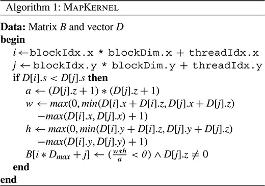
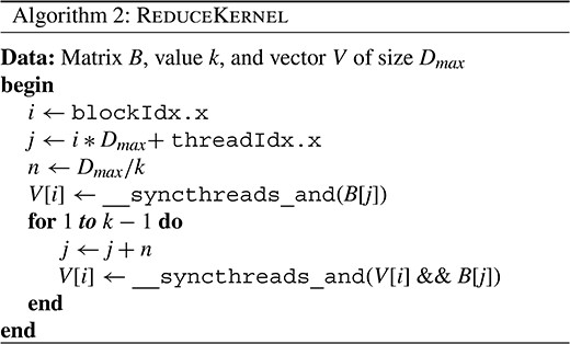
Figure 2 depicts a toy example of the proposed algorithm, in which an image frame contains three objects, three window clusters and nine detections. Our matrix encodes the relationship among all detections, initially assuming that all are possible cluster representatives (all matrix values are set to one after memory allocation). Therefore, a white color matrix element in Fig. 2 represents updated elements that were reset to Boolean true values (also, implemented using ones) while an element depicted in gray color means that the element has not been updated (original values that were set to one during initialization). Finally, an element depicted in black color means that it has been reconsidered as non-representative and replaced by a zero (Boolean false value).
Visualization of our GPU-NMS proposal: (a) example candidates generated by a detector (three objects, nine detections), Boolean matrix after (b) clustering and (c) cancellation of non-representatives and (d) result after AND reduction.
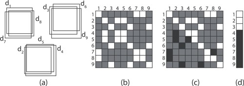
Firstly, we decide that two windows |$d_i$| and |$d_j$| belong to the same cluster if their areas are overlapped beyond a given threshold; otherwise, a zero will be placed in the matrix coordinates |$(d_i,d_j)$| and |$(d_j,d_i)$|. Secondly, we evaluate the non-zero values of each row, and again place zeroes if the row-indexed detection (|$d_i$|) is strictly smaller than the column-indexed one (|$d_j$|), thus discarding |$d_i$| as the cluster representative (blacked out in Fig. 2). Finally, a horizontal AND reduction will preserve a single representative per cluster, thus completing the NMS.
Formalizing this process, let |$D$| be the set of detection windows and |$C$| the set of clusters for a given frame, with |$C\subseteq D$|. We build a Boolean matrix |$B$| of size |$D_{max}\times D_{max}$|, being |$D_{max}$| an upper limit of the number of windows possibly generated by the detector at any frame. Let |$A(\cdot )$| be an operator that returns the area of a window. Given an overlapping threshold |$\theta \in \left [0,1\right ]$|, two candidate windows |$d_i$| and |$d_j$| are assigned to the same cluster if |$A(d_i\cap d_j)/A(d_i)\geq \theta $|. Candidates within a cluster are discarded as representatives if |$A(d_i)<A(d_j)$|. The clipping process is performed in parallel independently for each detection |$d\in D$| by a given computing thread. Since there are no data dependencies among detections, this mapping strategy scales properly as the amount of GPU cores is increased.
The only required parameters for this algorithm are the overlapping threshold |$\theta $| and the maximum number of possible candidates that can be generated by the detector |$D_{max}$|. Although this last constraint may initially seem to be an important drawback, in general conservative values for |$D_{max}$| turn to be very relaxed constraints. As an example, it is common that face detection models have a minimum face resolution of |$24\times 24$| pixels. In that case, the worst case scenario for a HD frame of |$1920\times 1080$| pixels would be a tiling of |$80\times 45$| faces of that size, yielding a matrix |$B$| of |$3600^2$| elements.
Internally, the map kernel (see the CUDA pseudocode in Algorithm 1) must first compute the area |$a$| to effectively perform the overlapping test for each pair of detections |$d_i, d_j \in D$|. With the aim of preserving simplicity, we assume equal width and height for the bounding boxes. Therefore, each detection is redefined as a |$\{x, y, z, s\}$| tuple, in which |$z=w=h$|.
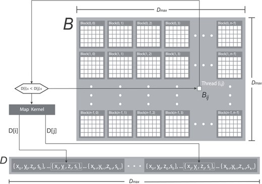
The process of constructing the Boolean |$B$| matrix is implemented by relying on a classic 2D parallelization pattern (see Fig. 3) in which each thread within a CUDA block updates a matrix element. Initially, all values of the |$B$| matrix are set to 1 by calling the cudaMemset() function before executing the map kernel to ensure the correctness of the algorithm. At this point, considering that the |$D$| vector constitutes a read-only input, it is possible to simultaneously access its values from multiple threads in the map kernel without relying on synchronization primitives for implementing the pre-clustering of detections according to their scores. Therefore, in Algorithm 1, the if statement checks |$D[i].s < D[j].s$| to ensure that a given block thread only updates a Boolean element |$B_{ij} \in B$| corresponding to a detection |$d_i \in D$| when its score is higher than the one of |$d_j \in D$|.
Representation of the NMS map kernel using the CUDA programming model notation.
An additional second conditional check is encoded as a Boolean expression in the kernel |$(\frac{w*h}{a} < \theta ) \wedge D[j].z \neq 0$| for re-tagging the |$B_{ij}$| element either as cluster candidate or non-candidate depending on the area overlap between |$d_i$| and |$d_j$|. The overlap is computed by means of |$max$| and |$min$| functions using as an input the |$x$| and |$y$| coordinates and the height and width of each |$(d_i,d_j)$| pair, whose dimensions depend only on its |$z$| component (|$z \times z$|). It also discards empty values of the |$D$| vector, as its size is allocated to an upper limit |$D_{max}$| that may not exactly match the total number of detections. This is ensured by the |$D[j].z \neq 0$| condition, which requires, as a prerequisite, all elements of the |$D$| vector initialized to 0 with cudaMemset() before storing on it the input detections to be merged by the NMS algorithm. Finally, the |$B_{ij}$| element is updated only if the overlapping ratio |$\frac{w*h}{a}$| exceeds the hand-crafted |$\theta $| threshold considered in the NMS process, as it happens with the conventional serial greedy NMS.
Once the Boolean matrix |$B$| has been computed, it is required to call a reduce kernel (see Algorithm 2) for selecting the optimal candidate from each row as it is depicted in Fig. 2. This task is performed using AND operations in parallel for each row of |$B$| and can be implemented in a CUDA kernel by means of __syncthreads_and(cond). This directive returns 1 only if the cond predicate evaluates to true for all threads of the CUDA block and is directly translated to the hardware-accelerated BAR.RED.AND assembly instruction. Therefore, it is possible to split the AND reductions of |$B$| by creating |$D_{max} / k$| partitions per row and then assigning each partition to a given thread block. As a proof of concept, Fig. 4 shows how the reduce kernel creates |$n$| CUDA blocks per partition (highlighted using dashed rectangles), thus precisely matching the number of rows of Boolean matrix |$B$|.
Illustration of the NMS reduce kernel showing partitions and CUDA blocks.
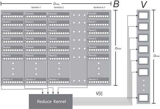
Under this parallelization pattern, threads are synchronized and simultaneously reduce the Boolean values stored in the CUDA block of each row partition by relying on the above-mentioned directive __syncthreads_and(V[i]). Partial row reductions of |$B$| are later stored in |$V[i]$|, a Boolean vector |$V$| of size |$D_{max}$|. Since we are dealing with a square matrix, it is required to call |$k$| times the reduction directive within the kernel assuming a CUDA block of size |$D_{max} / k$| and a grid size equal to the size of the |$D$| input set detections.
Consequently, after the first reduction ends, a for loop wraps up the remaining |$k-1$| reductions by calling __syncthreads_and() using as an input the partial AND reduction values stored in |$V[i]$|. An additional AND operation with the current thread block completes the operation (coded as |$B[j]$| && |$V[i]$|), effectively computing the correct aggregated reduction. On the other hand, parameter |$k$| must be experimentally determined so that the GPU achieves the highest occupancy and yields the minimum latency.
After having bitmasked all |$D$| vector elements with the Boolean values stored in |$V$|, the |$D_{\tiny \textsf{NMS}\normalsize }$| vector elements correspond to the merged set of detections (i.e. best representative of each cluster of detections). At this point, the execution of the parallel NMS algorithm is fully completed.
4. Algorithm Complexity
One of the goals of this study is to determine the time complexity of the kernels implementing the parallel NMS algorithm. In view of our kernels are meant to be executed on NVIDIA GPUs, which are mainly multithreaded data-parallel and throughput-oriented processors, their asymptotic time complexity must be determined using an idealized model of a parallel machine. In order to do so, we selected the parallel random-access machine (PRAM) model [26, 27], which is mainly an idealized shared address space parallel computer equipped with |$p$| processors lacking resource contention mechanisms. The generic PRAM model assumes that a given |$p$| processor has random access in unit time to any address of the external memory.
However, in order to realistically match a modern GPU, we selected a PRAM with concurrent read and concurrent write (CRCW) capabilities to the shared memory address space, as these particular read/write conflicts are usually managed by the programmer using the synchronization and atomic primitives offered by the CUDA programming model. It should be noted that the shared memory address space referred in the PRAM model corresponds to the global memory GPU address space (external DRAM) and not to the on-die shared memory included in the simultaneous multiprocessors (SMs) used in the standard CUDA-enabled GPU architecture.
The |$T_{\tiny \textsf{MAP}\normalsize }$| asymptotic cost shown in Equation 3 treats the |$p$| amount of processors as another variable in our analysis, in which |$p$| is expressed as a cost function of input |$n$|. This fact means that when Algorithm 1 is executed on a PRAM machine that has exactly enough |$p$| processors to exploit the maximum concurrency with |$n$| parallel operations, it behaves as a linear algorithm (i.e. |$T_{\tiny \textsf{MAP}\normalsize } = \Theta \left (n\right )$|).
Selected embedded NVIDIA Tegra platforms.
| Tegra SoC | CPU cores | CUDA cores | GPU architecture | GPU clock frequency |
|---|---|---|---|---|
| T124 | (4+1) Arm Cortex A15 | 192 | Kepler (GK20A) [sm_32] | 72 MHz – 852 MHz |
| T210 | (4) Arm Cortex A57 | 256 | Maxwell (GM20B) [sm_53] | 76.8 MHz – 998.4 MHz |
| T186 | (2) Denver2 + (4) Arm Cortex A57 | 256 | Pascal (GP10B) [sm_62] | 114.75 MHz – 1.3 GHz |
The asymptotic time complexity of the reduction kernel is summarized in Equation 4, and considering again a PRAM machine with |$p$| processors capable of computing |$n$| concurrent operations, |$T_{\tiny \textsf{REDUCE}\normalsize }$| could be simply approximated as |$\Theta \left (k\right )$|.
Although this time complexity analysis may be considered somewhat simplistic, as it does not take into account the capabilities of SM warp schedulers to issue and execute several warps concurrently nor considers the intrinsic low-level delays of the on-die GPU interconnect, it roughly highlights the computational burden of the two CUDA kernels. As a result, further experimentation and profiling on real platforms is required to determine the optimal |$k$| partition parameter and also to study the parallel NMS scalability as both the CUDA core count and the amount of objects to cluster is increased.
5. Evaluation Methodology
Several evaluations were conducted to precisely determine the latency of our proposed parallel NMS method. Since the main use case of such algorithm is to enable the clustering of a high number of simultaneous detections per frame on low-power embedded devices, the platforms selected for running the map/reduce kernels were the NVIDIA family of Tegra SoCs, which enable the scheduling, execution, profiling and debuggability of CUDA kernels with minimal efforts.
Tables 1 and 2 summarize the three boards used for running the experiments, as well as the version of the flashed NVIDIA JetPack image, which includes the required Linux for Tegra (L4T) OS distribution [28]. The source code of our kernels was compiled with NVIDIA’s nvcc compiler using the -O3 flag on each Tegra platform. This architectural diversity helped us on quantifying the scalability of the parallel algorithms implemented in our NMS kernels. More particularly, we were interested in benchmarking the NMS kernels across several generations of the Tegra SoCs featuring on-die GPUs with higher CUDA core counts, improved microarchitectures, memory bandwidth, bus width and clock frequencies.
Tested embedded boards, Linux distributions and CUDA runtime versions.
| Board | Tegra SoC | JetPack | L4T | CUDA |
|---|---|---|---|---|
| Jetson TK1 | T124 | v1.2 | R21.5 | 6.5 |
| Jetson TX1 | T210 | v3.2.1 | R28.2 | 9.0 |
| Jetson TX2 | T186 | v3.2.1 | R28.2 | 9.0 |
| Board | Tegra SoC | JetPack | L4T | CUDA |
|---|---|---|---|---|
| Jetson TK1 | T124 | v1.2 | R21.5 | 6.5 |
| Jetson TX1 | T210 | v3.2.1 | R28.2 | 9.0 |
| Jetson TX2 | T186 | v3.2.1 | R28.2 | 9.0 |
In order to do so, the clock rate of the GPU was manually set before each kernel execution by means of the Linux kernel pseudo filesystem device interface (sysfs). The path for setting the GPU frequency differed depending on the Tegra SoC model included in the embedded board (see Table 3). This low-level fine tuning opened us the door for comparing the throughput-oriented GPU architecture with the latency-oriented CPU cores when running both the conventional serial CPU-based NMS and the GPU-based parallel NMS at multiple clock frequencies.
sysfs path for setting up GPU clock rates.
| Tegra SoC | Filesystem path |
|---|---|
| T124 | /sys/kernel/debug/clock/gbus/ |
| T210 | /sys/devices/57000000.gpu/ |
| T186 | /sys/devices/17000000.gp10b/ |
| Tegra SoC | Filesystem path |
|---|---|
| T124 | /sys/kernel/debug/clock/gbus/ |
| T210 | /sys/devices/57000000.gpu/ |
| T186 | /sys/devices/17000000.gp10b/ |
The dynamic voltage and frequency scaling (DVFS) mechanisms of the CPUs were also disabled on purpose, and their corresponding clock frequencies manually set up for conducting a fair embedded CPU versus GPU comparison. Unfortunately, only the clustered multicore CPU design of the Tegra K1 SoC (T124) offered us the possibility of having access to an architecture packing high-performance out-of-order CPU cores with a low-performing and low-power CPU core (the so-called fifth companion core). The Tegra T210 SoC included in the Jetson TX1 board features only four high-performance Arm Cortex A57 CPU cores. Even though that the SoC die includes four additional in-order Arm Cortex A53 CPU cores, they were disabled on purpose during the manufacturing process. Therefore, this SoC does not provide OS-level access to a low-power cluster set of cores for reducing the power consumption when running background tasks, as opposed to other chips implementing Arm’s big.LITTLE technology [29].
On the other hand, the Tegra 186 SoC relies on a heterogeneous architecture that combines two high-performance Armv8-compliant VLIW cores developed by NVIDIA (Denver 2) with four out-of-order Arm Cortex A57 cores. Given that only the T124 SoC offered the possibility of running code at a true low-power CPU, we benchmarked the serial NMS code on the two CPU profiles available on that platform (i.e. high-performance CPU cores and the low-performance CPU core). Referring again to the GPU capabilities, even though that both T210 and T186 SoCs feature 256 CUDA cores, the latter one both runs at a higher clock rate and doubles the effective GPU memory bandwidth by increasing the memory bus from 64 bits to 128 bits. This fact will enable us later to study the impact of doubling the memory bandwidth when executing on the GPU the parallel map/reduce NMS kernels.
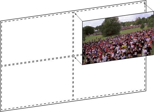
Synthetic 3840 x 2160 video frame from the mosaic dataset (post-NMS).
Finally, the most important part of the evaluation was to carefully select the input datasets to demonstrate how the proposed parallel NMS is able to cope with challenging real-world situations that feature lots of simultaneous objects in high-resolution images and video frames. As we are interested in human faces, we selected a 1080p input video from the SVT High Definition Multi Format Test Set1 (named crowd_run), which was originally filmed by the Swedish Television at 50 FPS using 65 mm film professional equipment. This particular video features approximately on average 60 simultaneous faces, but it was especially chosen because it yields hundreds of simultaneous detections per frame after having executed a CNN-based face classifier.
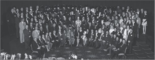
In order to further stress out the parallel NMS kernels, we post-processed the original 1080p crowd_run video stream to generate a 3960 x 2160 synthetic mosaic video incorporating four streams on each frame (depicted in Fig. 5), thus effectively quadrupling the number of simultaneous detected faces. Similarly, we also decided to study in detail the scalability of parallel NMS as the number of simultaneous faces are linearly increased. For this particular experiment, we selected a picture of the 83rd Academy Awards Nominees2 captured during the Oscars ceremony (named oscars in Table 4), which shows 147 simultaneous faces. Once all faces were detected, we coded and executed a script that generated 147 synthetic images from the original picture by covering and uncovering faces using rectangles filled with black color (see Fig. 6). Therefore, a given |$p_i$| picture (where |$1 \leq i \leq 147$|) would just uncover an additional face when compared to the previous |$p_{i-1}$| one. As an example, picture |$p_{0}$| starts the process by having all localized faces (147) covered with black rectangles to enforce the face classifier to yield zero detections. Under this rationale, picture |$p_{1}$| would cover 146 faces with black rectangles and uncover only a single face throughout the whole picture. As the script keeps going on generating synthetic images, picture |$p_{147}$| would conclude the process by showing all faces completely uncovered.
Input datasets selected for benchmarking the parallel NMS kernels.
| Input dataset | Resolution | Type |
|---|---|---|
| crowd_run | 1920 x 1080 | H.264 Video @ 50 FPS |
| mosaic | 3840 x 2160 | H.264 Video @ 50 FPS |
| oscars | 4646 x 1800 | JPEG Picture |
| Input dataset | Resolution | Type |
|---|---|---|
| crowd_run | 1920 x 1080 | H.264 Video @ 50 FPS |
| mosaic | 3840 x 2160 | H.264 Video @ 50 FPS |
| oscars | 4646 x 1800 | JPEG Picture |
Synthetic 83rd Academy Awards Nominees picture showing part of the faces covered.
6. Obtained Results
As it was previously discussed, first we started by determining how the latency of the GPU-based parallel NMS algorithm compares against the traditional serialized version of OpenCV’s |$\mathcal{O}(n^{2})$| greedy NMS, which is still used in many works [30] for clustering the bounding boxes obtained after inferencing CNN classifiers. This comparison was conducted by executing both NMS algorithms on the Jetson TK1 board using as an input the oscars dataset picture. More precisely, both NMS algorithms were executed at multiple frequencies on the two different CPU clusters available in the T124 SoC (i.e. high-performance CPU-G cluster and low-power CPU-LP cluster) by properly setting up the parameters in the sysfs Linux kernel interface. The CPU-LP core clock frequency ranges between 51 MHz and 1 GHz, while a given CPU-G core ranges between 204 MHz and 2.3 GHz. Similarly, the GPU clock ranges between 72 MHz and 850 MHz, as Table 1 shows. The results of this experiment are shown in Fig. 7.
NMS latency on GPU, CPU-LP and CPU-G cores for the selected oscars dataset.
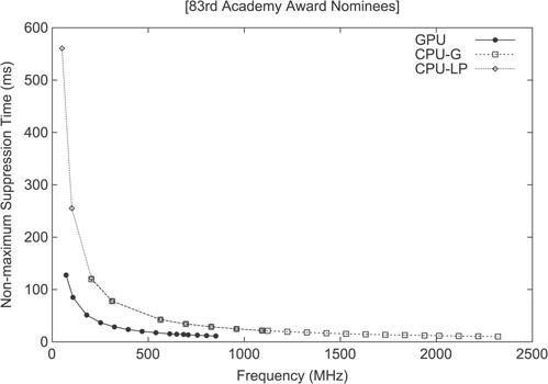
The graph clearly shows that a GPU clocked at 50% of its maximum frequency outperforms both CPU types also when they are operating at 50% of its peak operating frequency. For this experiment, the overhead of memory allocations and initializations was not taken into account and only the pure kernel execution time was considered. It should be noted that for battery-powered fanless solutions the chip must be underclocked or automatically managed by the underlying DVFS subsystem to avoid excessive overheating.
Unsurprisingly, the GPU shows an advantage, especially for GPU-based object detection and recognition pipelines, in which unwanted CPU/GPU memory transfers slowdown the throughput of real-time applications, as it would undesirably happen when relying on the serialized NMS targeting CPUs.
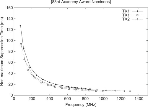
On the other hand, the proposed parallel NMS was evaluated on all GPUs of the selected Tegra platforms, also by varying the clock rate of the GPU before executing the kernels during the experiments, and using the same input dataset (oscars). The results of these experiments are summarized in Fig. 9. The reported latencies, aggregate the combined execution time of the map/reduce kernels within the parallel NMS algorithm, and shows a latency reduction improvement when scaling from 192 CUDA cores (Tegra T124) to 256 (Tegra T186 and T210). More precisely, the latencies obtained when running the kernels at the maximum GPU clock frequency were 11.24 ms (T124), 7.36 ms (T210) and 7.6 ms (T186), respectively, when clustering roughly 3000 simultaneous detections. Unexpectedly, although each experiment was executed three times to avoid the bias introduced by the CUDA runtime and scheduler, the obtained NMS algorithm performance was slightly faster on the Jetson TX1 board (T210) when compared to the results gathered on the Jetson TX2 (T186), which features a wider memory bus.
NMS latency on growing number of detections (oscars dataset).
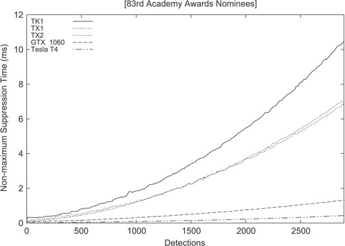
The obtained latency figures did not prove the general assumption that executing kernels on GPUs with equal core counts, but which differ in memory bandwidth and clock frequencies, would yield better performance results when physical specifications are improved across chip generations (see Table 1). Quite the contrary, it showed that for our proposed parallel NMS algorithm, it seems far more important to increase by a 33% the amount of GPU cores rather than simply increase the clock frequency and memory bandwidth, given a constant number of GPU cores. As an example, the T186 GPU must be clocked at 1.3 GHz to achieve the performance figures yielded by the T210 chip when clocked at 998.4 MHz. Therefore, the GPU scalability of parallel NMS is more sensitive to the number of cores (a 33% increase in GPU cores yields a 55% latency reduction), rather than to the improvements of the memory subsystem, thus highlighting that kernel code bottlenecks are skewed towards the availability and quantity of ALUs included in the GPUs (i.e. compute-bound kernel).
However, since the main benefit of the parallel NMS is the potential and flexibility offered for handling the clustering of detections in workloads featuring huge amounts of simultaneous objects, we decided to determine the scalability of the map/reduce kernels as the quantity of simultaneous faces are increased. These experiments involved the execution of the parallel NMS kernels on the selected Tegra platforms using as an input the synthetic set of pictures featuring covered faces (as it is shown in Fig. 6). The results of such experiments are summarized in the graph depicted in Fig. 8 and are consistent with the previous observation that emphasizes the importance of the GPU CUDA core count (both TX1 and TX2 outperform the older TK1). Hence, the slopes of both TX1 and TX2 graphs are greatly reduced when compared to the baseline TK1 graph, thus proving that our proposed parallel NMS algorithm properly scales as the CUDA core count is increased. In order to further illustrate this fact, Fig. 8 also shows an extra reduction of the graph slope when the parallel NMS algorithm is executed on a discrete NVIDIA GeForce GTX 1060 GPU featuring 1280 CUDA cores over a growing number of detections, and a further reduction when executed on a Tesla T4 GPU with 2560 CUDA cores. More particularly, the GTX 1060 yielded an 8.11X speed up over the TK1, 5.38X (TX2) and 5.23X (TX1), respectively. And the Tesla T4 yielded a 24.59X speed up over the TK1, 15.91X over TX2 and 16.44X over TX1.
NMS latency when processing the oscars dataset on the GPUs included in the selected Tegra SoCs.
As Table 5 shows, discrete GPUs clocked at roughly the same frequencies, and relying on comparable memory subsystem technologies (i.e. GDDR5 -GTX 1060- vs. GDDR6 -Tesla T4-), but with increased number of CUDA cores trigger substantial reductions in the NMS latency. As a result, increasing by a factor of 2 the amount of cores in the underlying hardware resources reduces the NMS execution latency by a factor of 3 for 2895 detections, effectively proving the scalability of our parallel NMS method as the amount of cores keeps increasing.
NMS latency on discrete GPUs when clustering n detections (oscars dataset).
| Discrete GPU | CUDA cores | Memory type | Clock rate | NMS latency (ms) | ||
|---|---|---|---|---|---|---|
| |$n = 200$| | |$n = 1027$| | |$n = 2895$| | ||||
| GeForce GTX 1060 | 1280 | GDDR5 | 1.70 GHz | 0.107 | 0.324 | 1.313 |
| Tesla T4 | 2560 | GDDR6 | 1.59 GHz | 0.024 | 0.088 | 0.430 |
| Discrete GPU | CUDA cores | Memory type | Clock rate | NMS latency (ms) | ||
|---|---|---|---|---|---|---|
| |$n = 200$| | |$n = 1027$| | |$n = 2895$| | ||||
| GeForce GTX 1060 | 1280 | GDDR5 | 1.70 GHz | 0.107 | 0.324 | 1.313 |
| Tesla T4 | 2560 | GDDR6 | 1.59 GHz | 0.024 | 0.088 | 0.430 |
These results are in line with our initial expectations about the time complexity of the parallel NMS. On these latter experiments, the GPU kernels were also compiled and benchmarked by setting |$k=32$| and |$D_{max}=4096$| (upper limit used for the GPU memory allocations required by matrix |$B$| and vector |$V$|).
In order to further study and optimize the NMS reduction kernel (Algorithm 2), several experiments were carried out to study the impact of parameter |$k$| with the aim of finding which partition size minimizes the latency in the NMS reduction kernel. Figure 11 summarizes the obtained results on each SoC of the selected Tegra platforms on the oscars dataset.
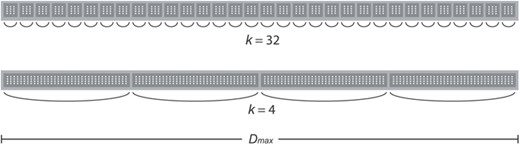
Thread synchronizations computed on a given B matrix row (k = 32 and k = 4).
NMS reduction kernel latency according to parameter k.
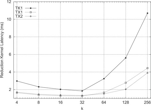
According to the experiments, the optimal partition size yielding minimal latencies would be |$k = 32$|, which was precisely the value used for obtaining the graph shown in Fig. 8. Interestingly, these results challenge conventional wisdom, as it is increasingly less costly to call |$k$| times __syncthreads_and() in the for loop when |$4 \leq k \leq 32$|. As thread synchronization is typically slow (i.e. theoretically, a barrier should be avoided if possible), it is considered counter-intuitive that an increasing number of thread synchronization operations could contribute to reduce the execution time. Taking into account that NVIDIA GPUs offer architectural support at the ISA level for implementing these primitives, and GPU hardware thread synchronization primitives work at the CUDA block level, the amount of |$D_{max} / k$| partitions created per matrix row effectively serves as a mechanism for fine-tuning the quantity of inter-block __syncthreads_and() calls executed in parallel (represented as arc symbols in Fig. 10). A comparison of the granularity of such thread synchronizations is highlighted in the aforementioned figure, which illustrates how the k parameter greatly affects the number of __syncthreads_and() calls executed in parallel, as the amount of CUDA blocks created varies. Nevertheless, when |$k> 32$|, as Fig. 11 depicts, the NMS reduction kernel latency keeps growing due to unoptimal CUDA block partitions when processing the input matrix |$B$|.
Finally, the crowd_run and mosaic datasets described in Table 4 were also used as an input of the map/reduce NMS kernels. The main objective of experimenting with those datasets was to characterize the underlying performance scalability of both kernels when localizing faces in videos featuring challenging real-world scenarios. Additionally, further experimentation was carried out to determine the execution time distribution of both Algorithm 1 (map kernel) and Algorithm 2 (reduce kernel).
As it was done with the oscars dataset picture, the NMS kernels were benchmarked over time on the selected Tegra platforms after having firstly decoded H.264 video frames and later performed face detection. The obtained results are summarized in Fig. 12, which shows both the number of faces detected per frame (top dashed line), and the aggregated latency of the parallel NMS kernels when executed on the selected SoCs (three lines shown at the bottom). Therefore, the H.264 decoding latency was not taken into account thus profiling only the map/reduce kernels at the low level.
NMS latency per frame vs. #det number of detections (crowd_run).
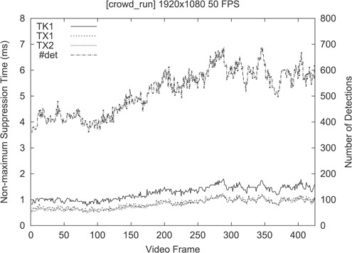
On this particular dataset (crowd_run), the amount of detected faces per frame ranged between 360 and 698 detections. Again, these experiments were carried out by setting |$k=32$| and |$D_{max}=4096$| when clustering detected faces. The aggregated latencies yielded by the parallel NMS were less than 2 ms. More particularly, it ranged between 0.5 and 1.8 ms when executed on the Jetson TK1 (T124). When switching to Jetson TX1 (T210) and Jetson TX2 (T186) platforms, latencies were reduced a further 50% due to the increased GPU core counts. As it also happened with previous experiments, there were no major performance improvements between TX1 and TX2 platforms when executing the parallel NMS algorithm. The latency reduction on TX2 was on average 6.25% lower than on TX1 and very close to 0.5 ms.
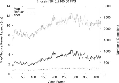
Therefore, in order to further spot differences and analyze the potential benefits of the improved T186 SoC, it might be necessary to saturate the GPU resources. Moreover, the mosaic video dataset was used as an input to quadruple the number of simultaneous detections per frame, so that the amount of thread reductions per row triggered by the NMS reduction kernel is greater than one. The results of these experiments are summarized in Table 6, which details the average latencies for both map and reduce kernels after having executed them on a frame per frame basis. Additionally, Table 6 reports how the execution time of the parallel NMS kernels was affected by parameter |$k$| on the selected Tegra platforms.
Average NMS latencies on TK1, TX1 and TX2 SoCs (mosaic dataset).
| Average NMS latency (ms) | ||||
|---|---|---|---|---|
| Tegra SoC | k | Map | Reduce | Total |
| TK1 | 4 | 5.17 | 2.41 | 7.78 |
| 8 | 5.16 | 1.87 | 7.22 | |
| 16 | 5.17 | 1.64 | 6.97 | |
| 32 | 5.17 | 1.54 | 6.88 | |
| TX1 | 4 | 3.74 | 1.34 | 4.84 |
| 8 | 3.37 | 1.11 | 4.57 | |
| 16 | 3.38 | 1.03 | 4.53 | |
| 32 | 3.38 | 1.00 | 4.48 | |
| TX2 | 4 | 3.52 | 1.37 | 4.93 |
| 8 | 3.50 | 1.16 | 4.71 | |
| 16 | 3.50 | 1.07 | 4.61 | |
| 32 | 3.49 | 1.03 | 4.56 | |
According to the obtained measurements, after quadrupling the amount of simultaneous faces, the main bottleneck of the parallel NMS algorithm lies on the construction of matrix |$B$|, which is performed in Algorithm 1 (map kernel). This performance penalty is noticeable in Fig. 13, as the depicted map kernel latency per frame seems proportional to the number of detected faces. These results are in line with the inner workings of Algorithm 1 since this kernel must populate |$n^2$| elements to cluster |$n$| detections. Consequently, it is the map kernel the one saturating the underlying hardware resources. On the other hand, the reduce kernel latency per frame remains roughly constant throughout the mosaic video frames, even when the number of simultaneous faces detected per frame is dramatically increased.
Map/reduce kernel latency per frame vs. #det number of detections (mosaic).
To conclude, we compared the accuracy of our parallel NMS method relying on the classic greedy approach to the recent NMS methods mentioned in Section 2. This comparison was conducted over the PASCAL VOC2007 and CrowdHuman datasets. For the algorithms lacking publicly available source code, we used the mAP and AP figures as reported by their respective authors when evaluating both datasets. The obtained results are summarized in Table 7, which clearly shows that alternative state-of-the-art NMS methods only marginal improve (between 1% and 2% in terms of mAP and AP depending on the dataset) the accuracy of our parallel NMS method. Moreover, alternative sequential methods applying minor variations to the classic greedy approach (i.e. AdaptiveNMS, Soft-NMS and FeatureNMS) could also be potentially adapted to GPU architectures using the parallelization techniques presented in Section 3.
Comparison between our parallel greedy NMS method and other state-of-the-art NMS methods on the PASCAL VOC2007 and CrowdHuman datasets.
| VOC2007 (mAP) | CrowdHuman (AP) | ||
|---|---|---|---|
| This work | 0.7516 | This work | 0.8307 |
| NMSNet [22] | 0.7659 | AdaptiveNMS [14] | 0.8471 |
| HS-NMS [24] | 0.7556 | FeatureNMS [15] | 0.8538 |
| Soft-NMS [13] | 0.7623 | Soft-NMS [13] | 0.8392 |
7. Algorithm Correctness
MapKernel(|$B$|, |$D$|) specification:
Precondition:|$D$| is a vector of unsorted detections of size |$D_{max}$|, and |$B[0...n-1][0...n-1]$| is a |$n \times n$| Boolean matrix in which all elements are set to true (represented with value 1). The dimensions of matrix |$B$| correspond to the size of vector |$D$| (|$n = D_{max}$|).
Postcondition:|$\forall i,j: 0 \leq i \leq n-1, 0 \leq j \leq n-1:$| A given |$B_{ij}$| element in Boolean matrix |$B$| encode if |$A(d_{i} \cap d_{j}) / A(d_{j}) < \theta $| and score(|$d_{i}$|) < score(|$d_{j}$|), in which detections |$d_{i},d_{j} \in D$|, and |$n = D_{max}$|.
The CUDA kernel pseudocode of Algorithm 1 meets the MapKernel(|$B$|, |$D$|) specification shown above, in which all threads created independently generate in parallel a single element of Boolean matrix |$B$|.
The input matrix |$B$| values are generated in parallel by creating |$D_{max} \times D_{max}$| threads using CUDA 2D block partitions of size blockDim * blockDim. This 2D parallelization pattern ensures that a given |$(i,j)$| thread generates only a single |$B_{ij}$| Boolean matrix element in the intervals |$0 \leq i \leq n-1$| and |$0 \leq j \leq n-1$|. As |$i,j$| indexes detections |$d_{i}$| and |$d_{j}$|, respectively; and the |$D$| vector is only accessed by threads within the kernel for read operations (i.e. never written), while |$B$| matrix values are never read by a thread, there is no chance for experiencing race conditions. Therefore, it is guaranteed that a given |$(i,j)$| thread will independently produce a single |$B_{ij}$| element as all D data dependencies are read-only and remain unmodified throughout the whole kernel execution. The |$i$| variable used in the kernel indexes |$B$| rows, whereas |$j$| is used to index the matrix columns. Hence, the kernel overwrites a given |$B_{ij}$| element only when the score of detection |$d_j$| exceeds the score of detection |$d_i$|. Due to the above-mentioned 2D parallelization pattern, when the kernel execution concludes, all possible detection pairs (|$d_i,d_j$|) derived from vector |$D$| will be compared against each other. On the other hand, |$w$| and |$h$| variables are set to the maximum width and height window dimensions of the considered (|$d_i,d_j$|) detection pair for computing the thresholded clipping process with |$\theta $| constant. As a result of this, the value stored in |$B_{ij}$| will be set with the Boolean obtained by evaluating the thresholded area intersection |$A(d_{i} \cap d_{j}) / A(d_{j}) < \theta $|. Therefore, after concluding the execution of the parallel kernel it is guaranteed that the postcondition is correctly met.
Precondition:|$B$| is |$n \times n$| Boolean matrix obtained after the execution of MapKernel, and |$V$| a Boolean vector o size |$n$| (|$n = D_{max}$|) in which all elements have been set to true. The |$k$| value is a parameter used to fine-tune the size of row partitions of matrix |$B$| when performing computations during kernel execution.
Postcondition:|$\forall i: 0 \leq i \leq n-1: V_i = \bigwedge _{j=0}^{n-1} (B_{ij})$| where |$n = D_{max}$|.
The kernel pseudocode of Algorithm 2 populates vector |$V$| by meeting the postcondition of ReduceKernel(|$B$|, |$k$|, |$V$|) described in the specification. The precondition must be satisfied by executing such kernel immediately after MapKernel(|$B$|, |$D$|).
8. Conclusions
In this paper, we have presented a novel highly scalable parallel NMS algorithm that is designed from scratch to handle workloads featuring thousands of simultaneous detections per frame. The proposed work-efficient NMS algorithm relies on a Boolean matrix, which is constructed element wise in parallel, and completes the cluster of detections by means of parallel reductions. Additionally, the input set of candidate windows does not require to be pre-sorted before running our method, as the proposed map kernel always selects the representative with the highest score among all detections within the cluster while building the Boolean matrix.
The obtained performance results show that the proposed map/reduce kernels are compute bound, and properly scale on embedded GPUs as the amount of CUDA cores is increased. As a result of this, the parallel NMS algorithm is capable of clustering 1024 simultaneous detected faces per frame in roughly 1 ms on both Tegra X1 (T210) and Tegra X2 (T186) on-die GPUs, while taking 2 ms on Tegra K1 (T124). Therefore, the parallel NMS execution time is effectively reduced 53% when the GPU computing resources are increased by a 33% from 192 to 256 CUDA cores. Thanks to additional experimentation, we also proved that this ratio is further improved as the amount simultaneous detections per frame keeps growing (e.g. 2048 detections and beyond).
Moreover, when the proposed parallel NMS method is executed on powerful discrete GPUs with high core counts and complex memory hierarchies, the execution time is even more drastically reduced. Interestingly, our obtained results show that doubling the amount of cores from 1280 to 2560 reduces the NMS execution time by at least a factor of three, which is even more pronounced than in the embedded GPU platforms. In this latter scenario, the parallel NMS is capable of clustering roughly 3000 candidate windows in less than 0.5 ms. These results show that our NMS method yields a minimal footprint in a GPU-only object recognition pipeline, as its execution consumes only 1% of the hard deadline of the 40 ms required for the real-time processing of video feeds at 25 FPS.
On the other hand, the proposed kernels do not require to perform any GPU-to-CPU and CPU-to-GPU memory transfers, as the input of the map kernel is directly populated with the output of a GPU-based object detection framework, thus involving only GPU-to-GPU memory transfers. Similarly, output data obtained after the execution of the map kernel is directly fed to the input of the reduce kernel within the GPU memory address space. This fact means that our parallel NMS method is the perfect solution for implementing an object recognition pipeline completely offloaded to GPU architectures.
Regarding accuracy, as we do not modify the inner workings of the conventional sequential greedy NMS method, our parallel algorithm remains highly competitive [13]. Furthermore, recent variations of the serial-based greedy NMS algorithm [14, 15] could also benefit from the scalability of the parallelization pattern and implementation studied in this paper.
Other alternatives, such as state-of-the-art learning-based methods, which require inferencing an additional CNN for solving the NMS problem, improve at most a 2% [19, 22] the AP when compared to the classic NMS method, but dramatically increase both the computational burden and latency (|$\sim $|14x in [19] and |$\sim $|40x in [22]), which is key for real-time applications.
As future work, we plan to study the performance impact of implementing thread group synchronization in the reduction kernel grid. However, as this feature is only available on Pascal, Volta, and Ampere GPU architectures, it would sacrifice portability of the parallel NMS kernel across legacy GPU computing platforms.
Funding
Ministerio de Economía y Competitividad under contracts (TIN2015-65316-P, TEC2012-38939-C03-02); the Departament d’Innovació, Universitats i Empresa de la Generalitat de Catalunya under project MPEXPAR: Models de Programació i Entorns d’Execució Paral|$\cdot $|lels (2014-SGR-1051); and the European Commission under the Horizon 2020 program (H2020-ICT-644312).
Footnotes
References
