


SUMMARY
The euro crisis was fuelled by the diabolic loop between sovereign risk and bank risk, coupled with cross-border flight-to-safety capital flows. European Safe Bonds (ESBies), a euro area-wide safe asset without joint liability, would help to resolve these problems. We make three contributions. First, numerical simulations show that ESBies with a subordination level of 30% would be as safe as German bunds and would increase safe asset supply. Second, a model shows how, when and why the two features of ESBies – diversification and seniority – can weaken the diabolic loop and its diffusion across countries. Third, we propose how to create ESBies, starting with limited issuance by public or private-sector entities.
1. INTRODUCTION
The creation of the euro in 1999 was a landmark in the European integration process. Since 2009, however, the euro area has been roiled by financial crisis, with heightened sovereign default risk, a weakened banking sector, and a stagnating macroeconomy.
Why did this happen? Among many factors, the euro area lacked institutional features necessary for the success of a monetary union, including emergency funding for sovereigns and common banking supervision and resolution (Brunnermeier et al., 2016). Some of these deficiencies have since been addressed, but one crucial feature remains missing. The euro area does not supply a union-wide safe asset, i.e. one that yields the same pay-off at any point in time and state of the world (Section 2). By storing value in safe assets, rather than the risky debt of the nation-state in which they reside, banks would weaken the diabolic loop between their solvency and that of their domestic government. In a cross-border currency area, union-wide safe assets ensure that flight-to-safety capital flows occur across assets (i.e. from risky to risk-free assets) rather than countries.
To fill this gap, Brunnermeier et al. (2011) propose Sovereign Bond-Backed Securities (SBBSs), which constitute senior and junior claims on a diversified portfolio of euro area central government (‘sovereign’) bonds (Section 3). SBBSs are politically feasible as they entail no joint liability among sovereigns, in contrast to most other proposals.1 Governments remain responsible for servicing their own debt, which trades at a market price, exerting discipline on borrowing decisions. One government could default on its obligations without others bearing any bail-out responsibility and without holders of the senior claim bearing any losses.
We advocate Brunnermeier et al.’s proposal in three ways. First, in Section 4, simulations measure SBBSs’ risk. With a subordination level of 30%, the senior claim has an expected loss rate similar to that of German bunds. This motivates the moniker of ‘European Safe Bonds’ (or ‘ESBies’) to refer to the senior claim. In addition, ESBies would increase the supply of safe assets relative to the status quo. The corresponding junior claim — which we refer to as ‘European Junior Bonds’ (or ‘EJBies’) — would be attractive investments, thanks to their embedded leverage and expected loss rates similar to those of riskier euro area sovereign bonds.
These simulations take default probabilities as given, yet probabilities should change endogenously in response to banks’ safer portfolios. To capture this idea, in Section 5, we extend a workhorse model of the diabolic loop between sovereign risk and bank risk developed by Brunnermeier et al. (2016). We show that the diabolic loop is less likely to arise if banks hold adequately subordinated ESBies rather than domestic government debt or a diversified portfolio with no tranching. ESBies are thus a ‘positive sum game’.
Third, in Sections 6 and 7, we investigate how to implement ESBies. At present, their creation is stymied by regulation, which would penalize them relative to direct holdings of sovereign bonds. To remove this regulatory roadblock, policy-makers should ensure a fair treatment of ESBies, and provide incentives for greater diversification of banks’ and insurers’ government debt portfolios. Policy should also play a standard-setting role, helping financial institutions to overcome coordination failures in creating a new market. An official Handbook should define ESBies’ subordination level and underlying portfolio composition, as well as the institution(s) licensed to issue them. Following these preparatory steps, issuance should start at a small scale, allowing investors to digest the new securities, before the market for ESBies is deepened.
2. CRISIS WITHOUT A UNION-WIDE SAFE ASSET
Modern financial systems rely on safe assets. They lubricate financial transactions, which often entail a contractual requirement to post collateral (Giovannini, 2013), and so allow market participants to transfer liquidity or market risk without creating counterparty credit risk. To comply with liquidity regulations, banks need to hold safe assets to meet their funding needs in a stress scenario (Basel Committee on Banking Supervision, 2013). And central banks conduct monetary policy by exchanging money, whether currency or reserves, for quasi-money in the form of safe assets with longer maturities (Brunnermeier and Sannikov, 2016).
A safe asset is liquid, maintains value during crises, and is denominated in a currency with stable purchasing power. Relative to investors’ demand for safe assets, there is scarce global supply of securities that possess all three characteristics (Caballero, 2010). The most widely held safe asset, US Treasury bills and bonds, earns a large ‘safe haven’ premium of 0.7% per year on average (Krishnamurthy and Vissing-Jorgensen, 2012). Acute safe asset scarcity can have negative macroeconomic effects by increasing risk premia, pushing the economy into a ‘safety trap’ (Caballero et al., 2016).
The euro area does not supply a safe asset on par with the United States, despite encompassing a similarly large economy and developed financial markets. Instead, euro area governments issue debt with heterogeneous risk and liquidity characteristics. Five euro area nation-states – Germany, the Netherlands, Austria, Finland and Luxembourg – are rated triple-A by either Moody’s or S&P. In 2015, the face value of central government debt securities issued by these nation-states stood at €1.9tn (18% of euro area GDP). By contrast, outstanding central government debt securities issued by the United States had a face value of $11.7tn in 2015 (65% of US GDP). The relative scarcity and asymmetric supply of euro-denominated safe assets creates two problems, which we explain next.
2.1. Diabolic loop
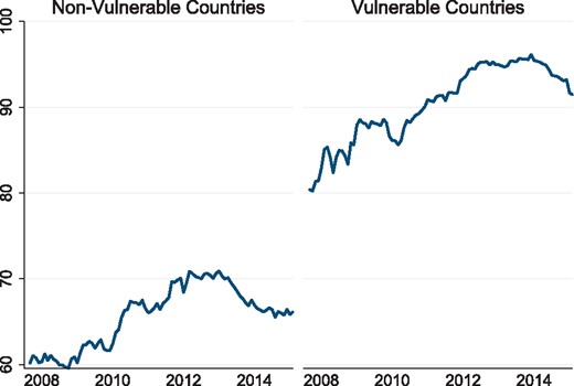
Mean of banks’ domestic sovereign bond holdings as a percentage of their total holdings
Notes: Figure plots the mean of euro area banks’ holdings of their own sovereign’s debt as a proportion of their total sovereign debt holdings. Banks are split into two subsamples: those resident in ‘non-vulnerable’ countries (i.e. Austria, Belgium, Germany, Estonia, Finland, France, Luxembourg, Malta, the Netherlands) and those in ‘vulnerable’ countries (i.e. Spain, Ireland, Italy, Portugal, Cyprus, Slovenia, Greece).
Sources: ECB; Altavilla et al. (2016).
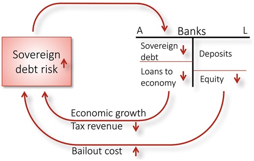
The sovereign-bank diabolic loop
Notes: Figure depicts the diabolic loop between sovereign risk and bank risk. The first loop operates via a bail-out channel: the reduction in banks’ solvency raises the probability of a bail-out, increasing sovereign risk and lowering bond prices. The second loop operates via the real economy: the reduction in banks’ solvency owing to the fall in sovereign bond prices prompts them to cut lending – reducing real activity, lowering tax revenues and increasing sovereign risk further.
Source: Brunnermeier et al. (2011).
This loop was the quintessential characteristic of the euro area sovereign debt crisis. In some countries (e.g. Ireland and Spain), widespread bank insolvencies endangered the sustainability of sovereign debt dynamics. In other countries – Greece, Italy, Portugal and Belgium – long-run public debt accumulation and slow growth generated sovereign debt dynamics that threatened banks’ solvency. In both cases, domestic governments’ guarantees became less credible, and the interaction of sovereign risk and bank risk amplified the crisis after 2009. To weaken the diabolic loop, the euro area needs a safe asset that banks can hold without being exposed to domestic sovereign risk.
2.2. Flight to safety
The euro area features a strong asymmetry in the provision of safe assets: Germany supplies two-thirds of top-rated euro-denominated central government debt securities. This asymmetry exacerbates the swings of cross-border capital flows during financial crises.
During the 2003–2007 boom, capital flowed from non-vulnerable to vulnerable countries, attracted by the perceived relative abundance of investment opportunities and the absence of foreign exchange risk. These boom-era capital flows fuelled credit expansion in vulnerable countries, raising local asset prices and compressing sovereign bond spreads. Effectively, investors treated all euro area nation-states’ bonds as safe. In the presence of financial frictions, however, the credit expansion in vulnerable countries led to an appreciation of the real exchange rate. Productivity slumped because extra credit was disproportionately allocated to low-value-added sectors (Reis, 2013), especially real estate and other non-tradable sectors (Benigno and Fornaro, 2014).
After 2009, short-term capital flows from non-vulnerable to vulnerable countries reversed, as investors sought safety above all else (Lane, 2013). Without a union-wide safe asset, non-vulnerable sovereigns’ debt partially satisfied investors’ newfound demand for safety. The capital flow reversal depressed non-vulnerable nation-states’ borrowing costs below the level justified by fundamentals – and, in proportion, elevated vulnerable sovereigns’ borrowing costs. Consequently, capital in search of safety flowed from high-risk to low-risk countries in a self-fulfilling manner.
With ESBies, capital flights to safety would take place from high-risk to low-risk European assets rather than from vulnerable to non-vulnerable countries. As a result, the safe haven premium enjoyed during crises by the euro area’s pre-eminent safe asset – German bunds – would dissipate. This dissipation is desirable: Germany’s safe haven premium is the corollary of expectations-driven runs on sovereign debt elsewhere in the euro area. From a German point of view, the loss of the safe haven premium would be compensated in two ways. First, ESBies would reduce the probability of crises, as we show in Section 5. Crises are particularly damaging for Germany’s export-oriented economy, regardless of the safe haven premium. Second, conditional on being in a crisis, bail-out requirements would be smaller if banks’ portfolios were invested in ESBies, as they would be less exposed to sovereign risk. This benefits fiscally strong countries that might otherwise contribute disproportionately to a bail-out.
3. DESIGN OF ESBies
ESBies are the senior claim on a diversified portfolio of euro area sovereign bonds. To create them, a public or private special purpose entity (or entities) purchases a diversified portfolio of euro area sovereign bonds,2 weighted according to a moving average of euro area countries’ GDPs or contributions to European Central Bank (ECB) capital.3 For investors, a well-defined, slow-moving weighting scheme has the benefit of transparency and predictability. More importantly, the use of GDP or ECB capital key weights ensures that there are no perverse incentives for governments in terms of debt issuance: the special purpose entity or entities would buy only a certain fraction of each country’s outstanding central government debt securities at their market price. Countries with large debt stocks would need to place proportionally more of their obligations in the open market.4
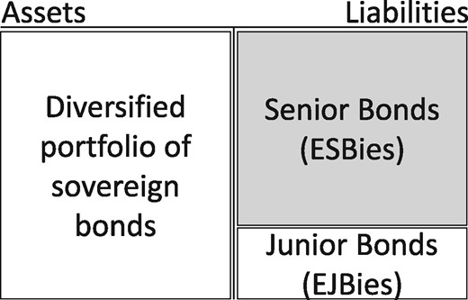
Balance sheet of an SBBS securitization vehicle
Notes: Figure shows the balance sheet of an SBBS securitization vehicle, whereby its diversified portfolio of sovereign bonds is financed by the issuance of two securities, with ESBies senior to EJBies.
Both tranching and diversification are key to ESBies’ safety. Losses arising from sovereign defaults would first be borne by holders of the junior bond; only if they exceed the subordination level, such that EJBies are entirely wiped out, would ESBies begin to take any losses. In Section 4, we show that a subordination level of 30% – such that the junior bond represents 30%, and the senior bond 70%, of the underlying face value – would ensure that ESBies have an expected loss rate similar to that of German bunds. As such, ESBies would be standard low-risk fixed income securities; EJBies would be more akin to government equity with a state-contingent pay-off structure. The next sections explore the quantitative properties of ESBies and EJBies, their effect on the diabolic loop, and their practical implementation.
4. QUANTITATIVE PROPERTIES OF ESBies
This section addresses three related questions. Would ESBies be as safe as top-rated sovereign bonds? Would their supply be adequate for banks to use them as a safe store of value? And would there be enough demand for EJBies? The simulation results lead us to answer ‘yes’ to all three questions. First, with an appropriate subordination level, ESBies can be designed such that they are as safe as German sovereign bonds. Second, ESBies could substantially increase the supply of safe assets relative to the status quo, without deviating from the fundamental principle that they should be backed by the sovereign bonds of all euro area Member States (with the exception of those which have lost primary market access, as we explain in Subsection 6.2.3). Third, in our benchmark calibration, EJBies have an expected loss rate comparable to those of vulnerable euro area sovereign bonds.
We obtain these results by comparing four security designs: (i) the status quo, in which sovereign bonds are neither pooled across nation-states nor tranched for safety; (ii) national tranching, where each sovereign bond is tranched into a senior and junior component at a given subordination level; (iii) pure pooling, where sovereign bonds are pooled in a single portfolio, with weights equal to countries’ relative GDP over 2010–2014; and (iv) pooling and tranching, where the pooled portfolio is tranched into a senior component (ESBies) and a junior component (EJBies) at a given subordination level.
We begin with a simple calculation to illustrate ESBies’ robustness to extreme default scenarios (Subsection 4.1). We then undertake a more rigorous analysis by way of numerical simulations (Subsection 4.2). Under a benchmark calibration of the simulation model, ESBies with a subordination level of 30% are as safe as German bunds (Subsection 4.3). To check the sensitivity of these results to parameter uncertainty, which is a perennial concern when measuring the risk of securitizations (Antoniades and Tarashev, 2014), we subject the simulation model to an adverse calibration in Subsection 4.4 and a battery of alternative parameterizations in a separate Web Appendix.
These simulations take the distribution of default and loss-given-default (LGD) rates as given, and therefore, ignore general equilibrium effects. Yet by expanding the volume of safe assets that may be held by banks, ESBies endogenously reduce the number of states in which the diabolic loop can operate. Because this mechanism is hard to quantify empirically, Section 5 presents a theoretical model that captures it. For now, though, by neglecting this general equilibrium effect, our simulations are conservative in the sense that they understate the risk reduction that ESBies can achieve.
4.1. Illustrative default scenarios
Sovereign defaults are rare events, implying considerable uncertainty regarding true LGD rates. For robustness, we subject sovereign bonds to three different LGD rates per country i: and . The values of , which represent the most severe losses, are shown in Table 1; the values of are 80% those of ; and values are 50% lower.
Simulation inputs
| (1) | (2) | (3) | (4) | (5) | (6) | (7) | (8) | |
|---|---|---|---|---|---|---|---|---|
| Rating | C. Bonds/GDP | G. Debt/GDP | Weight | pd1 | pd2 | pd3 | lgd1 | |
| Germany | 1 | 39 | 71 | 28.16 | 5 | 0.5 | 0 | 40 |
| The Netherlands | 1 | 51 | 65 | 6.61 | 10 | 1 | 0 | 40 |
| Luxembourg | 1 | 12 | 22 | 0.18 | 10 | 1 | 0 | 40 |
| Austria | 1.5 | 67 | 86 | 3.21 | 15 | 2 | 0 | 45 |
| Finland | 1.5 | 48 | 64 | 2.02 | 15 | 2 | 0 | 45 |
| France | 3 | 73 | 96 | 21.25 | 25 | 3 | 0.05 | 60 |
| Belgium | 3.5 | 84 | 106 | 3.93 | 30 | 4 | 0.1 | 62.5 |
| Estonia | 4.5 | 0 | 10 | 0.03 | 35 | 5 | 0.1 | 67.5 |
| Slovakia | 5 | 45 | 52 | 0.66 | 35 | 6 | 0.1 | 70 |
| Ireland | 6.5 | 49 | 79 | 1.80 | 40 | 6 | 0.12 | 75 |
| Latvia | 7 | 25 | 36 | 0.17 | 50 | 10 | 0.3 | 75 |
| Lithuania | 7 | 34 | 43 | 0.25 | 50 | 10 | 0.3 | 75 |
| Malta | 7.5 | 56 | 61 | 0.07 | 55 | 11 | 0.4 | 78 |
| Slovenia | 9 | 71 | 83 | 0.37 | 60 | 15 | 0.4 | 80 |
| Spain | 9 | 79 | 100 | 10.77 | 60 | 15 | 0.4 | 80 |
| Italy | 9.5 | 110 | 132 | 16.52 | 65 | 18 | 0.5 | 80 |
| Portugal | 12 | 72 | 129 | 1.77 | 70 | 30 | 2.5 | 85 |
| Cyprus | 13.5 | 35 | 108 | 0.19 | 75 | 40 | 10 | 87.5 |
| Greece | 19 | 40 | 177 | 2.01 | 95 | 75 | 45 | 95 |
| Average | 4.6 | 66 | 93 | 31.30 | 8.07 | 1.12 | 59.47 | |
Notes: This table reports the inputs used in the numerical simulations described in Section 4. Nation-states are ordered in terms of their sovereign credit ratings as of December 2015. Letter grades are converted into a numerical score (1 is AAA, 19 is CCC-) and averaged across S&P and Moody’s (column 1). Column 2 refers to the face value of outstanding central government debt securities as a percentage of GDP in Q4 2015 (Eurostat code: gov_10q_ggdebt). Column 3 refers to the face value of consolidated general government gross debt (following the Maastricht criteria) as a percentage of GDP in 2015 (Eurostat codes: teina225 and naida_10_gdp). Column 4 refers to the percentage weight of each sovereign in the pooled euro area portfolio, corresponding to nation-states’ relative GDPs (with the constraint that the pooled portfolio cannot include more than 100% of nation-states’ outstanding debt). Columns 5–7 describe the five-year default probabilities (in percentage) in states 1, 2 and 3, respectively. Column 8 describes the five-year LGD rates (in percentage) in state 1; in state 2, LGD rates are 80% of those in state 1 and in state 3 they are 50% of those in state 1.
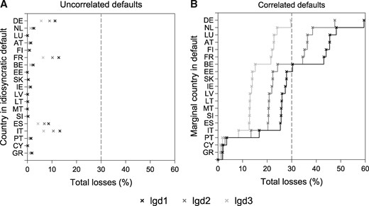
Illustrative default scenarios
Notes: Figure plots total losses incurred by a portfolio comprising euro area sovereign bonds with weights given in Table 1. Panel A plots total losses on this portfolio following uncorrelated, country-specific default events (under the respective LGD of and , shown in different shades of grey, and given in Table 1). Panel B plots total losses following simultaneous cross-country defaults: at any given point on the vertical axis, all countries at and below that point are assumed to be in default.
In Panel B of Figure 4, defaults are correlated across countries. At any given point on the vertical axis, all countries at and below that point are assumed to be in default, with loss rates given by their respective or . For example, the ‘ES’ point on the vertical axis refers to simultaneous defaults by Spain, Italy, Portugal, Cyprus and Greece: when this happens, the underlying portfolio incurs losses of 25.4%, 20.3% or 12.7% under assumptions of and , respectively. With , ESBies are robust to simultaneous defaults by Estonia and all nation-states rated below it; with , they are robust to defaults by France and all nation-states rated below it; with , they survive all defaults (i.e. ESBies incur no losses even if all nation-states default).
These illustrative calculations are informative regarding the severity of shocks that would be necessary for ESBies to begin to take any losses. Their usefulness is limited, however, as they consider a set of default events without specifying their probabilities. Therefore, in the next subsection, we subject ESBies and EJBies to an ex ante risk assessment in a simulation model, which takes thousands of draws from default probability distributions.
4.2. Simulating multiple default scenarios
To further assess the quantitative properties of ESBies and EJBies, we design a two-level hierarchical simulation model. In the first level, we simulate 2,000 five-year periods, in each of which the aggregate economic state can take one of three values:
State 1: A severe recession occurs; default and LGD rates are very high for all nation-states, and particularly for those with worse credit ratings. In this state, the expected default rate over five years is listed in column 5 of Table 1; LGD rates are shown in column 8.
State 2: A mild recession occurs; default and LGD rates are elevated in all nation-states. Expected five-year default rates are given in column 6 of Table 1; expected LGD rates are 80% of those in state 1.
State 3: The economy expands; default risk is low for most nation-states (column 7 of Table 1); LGD rates are 50% of those in state 1.
The aggregate random variable determines that the euro area economy is in the good state 70% of the time and in one of the two recessionary states 30% of the time. This 70:30 split between expansions and recessions accords with NBER data on the US business cycle spanning 1854–2010. Using CEPR’s business cycle dating for the euro area on the shorter sample of 1974–2014, the economy was in a recession in 20% of the years, so our assumption of 70:30 is appropriately pessimistic. Of the 30% recessionary states, similarly long time-series data gathered by Reinhart and Rogoff (2009) and Schularick and Taylor (2012) suggest that about one-sixth are severe. We match these historical patterns by assuming that mild recessions occur 25% of the time and severe recessions occur 5% of the time.
The model’s second hierarchical level concerns sovereign default. Within each five-year period, conditional on the aggregate state in that period (drawn in the first level of the model), we take 5,000 draws of the sovereigns’ stochastic default processes. The random variable that determines whether a given sovereign defaults, and which can be interpreted as the ‘sunspot’ in the theoretical model of Section 5, is assumed to have a fat-tailed distribution (Student’s t with four degrees of freedom), making defaults far more likely than under a normal distribution. In each state of the economy, nation-states’ default probabilities increase with their numerical credit score (higher scores indicate worse ratings). With 2,000 five-year periods and 5,000 draws within each period, our simulation uses a total of 10 million draws.
4.3. Benchmark calibration of the numerical simulation
The purpose of our simulations is to compare the four cases of security design along two dimensions: five-year expected loss rates (calculated as average loss rates over the simulations of the default process), and the ‘safe asset multiplier’ (namely the units of safe assets produced by the securitization per unit of safe asset in the underlying portfolio).
In the benchmark calibration of the model, we select the parameters such that average default rates are consistent with market prices. According to calculations by Deutsche Bank, which infers default probabilities from credit default swap (CDS) spreads by assuming a constant LGD rate of 40%, annual default probabilities were 0.20% for Germany and 0.30% for the Netherlands in December 2015; by comparison, our benchmark calibration of the model calculates 0.07 and 0.15%, respectively. This difference can be explained by the counterparty credit risk and liquidity premia that inflate CDS spreads, particularly for highly rated reference entities. For other countries, our model calculates precisely the same default probabilities as those implied by CDS spreads in December 2015. This cross-check with CDS spreads allows us to establish nation-states’ relative riskiness; in Subsection 4.4 and the Web Appendix, we subject default rates to various stress tests.
Moreover, the model is calibrated so that LGD rates are broadly consistent with historical data on recoveries following sovereign defaults. According to Moody’s data on sovereign defaults over 1983–2010, most of which were by emerging or developing economies, issuer-weighted LGD rates were 47% when measured by the post-default versus pre-distress trading price, and 33% based on the present value of cash flows received as a result of the distressed exchange compared with those initially promised. On a value-weighted basis, average LGD rates were 69% and 64%, respectively. This calibration is subject to further robustness checks in the Web Appendix, where we envisage a uniform 15% increase in LGD rates.
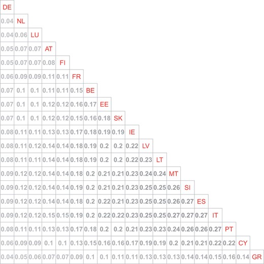
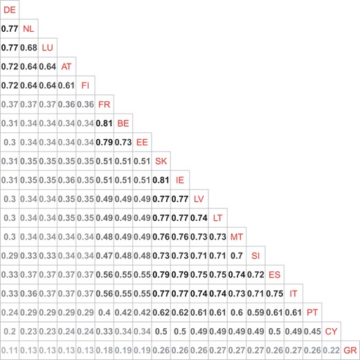
These calibrations deliver the default and LGD rates reported in Table 1, and the cross-country correlations in default probabilities shown in Panel A of Table 2. Later, in Subsection 4.4, we impose additional contagion assumptions that lead to the aggravated correlations shown in Panel B of Table 2. Even more severe contagion assumptions are modelled in the Web Appendix.
Correlations between nation-states’ default probabilities
| Panel A: Benchmark calibration | ||||||||||||||||||
 | ||||||||||||||||||
| Panel B: Adverse calibration | ||||||||||||||||||
 |
| Panel A: Benchmark calibration | ||||||||||||||||||
| ||||||||||||||||||
| Panel B: Adverse calibration | ||||||||||||||||||
|
Notes: Matrices show the correlations between nation-states’ probabilities of default in the benchmark (Panel A, described in Subsection 4.3) and adverse (Panel B, described in Subsection 4.4) calibrations of the simulation model. Correlations are much higher in the adverse calibration owing to the additional contagion assumptions. Higher (lower) correlations are shown in darker (lighter) gray.
Correlations between nation-states’ default probabilities
| Panel A: Benchmark calibration | ||||||||||||||||||
| ||||||||||||||||||
| Panel B: Adverse calibration | ||||||||||||||||||
|
| Panel A: Benchmark calibration | ||||||||||||||||||
| ||||||||||||||||||
| Panel B: Adverse calibration | ||||||||||||||||||
|
Notes: Matrices show the correlations between nation-states’ probabilities of default in the benchmark (Panel A, described in Subsection 4.3) and adverse (Panel B, described in Subsection 4.4) calibrations of the simulation model. Correlations are much higher in the adverse calibration owing to the additional contagion assumptions. Higher (lower) correlations are shown in darker (lighter) gray.
4.3.1. Effects of pooling and tranching on safety
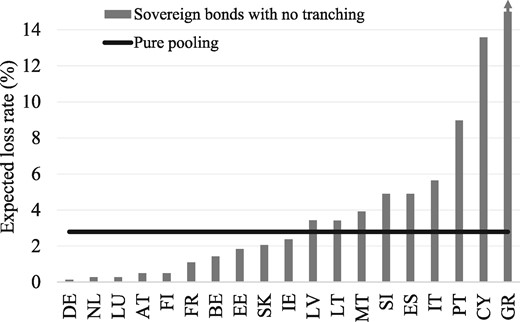
Untranched bonds’ five-year expected loss rates
Notes: Figure shows the expected loss rates of national sovereign bonds versus that of the pooled euro area security without tranching. The vertical axis is truncated at 15% for presentational purposes; the expected loss rate on Greek sovereign bonds is 34.16%. The data presented in this figure correspond to those reported in Table 3.
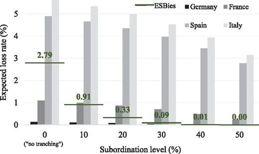
Senior bonds’ five-year expected loss rates by subordination level
Notes: Figure shows the expected loss rates of the senior tranche of national sovereign bonds versus that of the pooled euro area security. When the subordination level is 0%, there is no tranching: national sovereign bonds correspond to the status quo, and the pooled security corresponds to pure pooling (as in Figure 5). When the subordination level is greater than 0%, national sovereign bonds correspond to national tranching, and the pooled portfolio corresponds to ESBies. For brevity, this figure displays only the largest four nation-states; data for others are shown in Table 3.
Senior bonds’ five-year expected loss rates in the benchmark calibration (%)
| Subordination | 0% | 10% | 20% | 30% | 40% | 50% | 60% | 70% | 80% | 90% |
|---|---|---|---|---|---|---|---|---|---|---|
| Germany | 0.13 | 0.11 | 0.08 | 0.04 | 0.00 | 0.00 | 0.00 | 0.00 | 0.00 | 0.00 |
| The Netherlands | 0.27 | 0.22 | 0.15 | 0.07 | 0.00 | 0.00 | 0.00 | 0.00 | 0.00 | 0.00 |
| Luxembourg | 0.27 | 0.22 | 0.15 | 0.07 | 0.00 | 0.00 | 0.00 | 0.00 | 0.00 | 0.00 |
| Austria | 0.50 | 0.42 | 0.32 | 0.19 | 0.06 | 0.00 | 0.00 | 0.00 | 0.00 | 0.00 |
| Finland | 0.50 | 0.42 | 0.32 | 0.19 | 0.06 | 0.00 | 0.00 | 0.00 | 0.00 | 0.00 |
| France | 1.09 | 0.99 | 0.86 | 0.70 | 0.49 | 0.23 | 0.00 | 0.00 | 0.00 | 0.00 |
| Belgium | 1.42 | 1.29 | 1.14 | 0.94 | 0.69 | 0.34 | 0.09 | 0.00 | 0.00 | 0.00 |
| Estonia | 1.83 | 1.70 | 1.53 | 1.32 | 1.05 | 0.67 | 0.30 | 0.00 | 0.00 | 0.00 |
| Slovakia | 2.05 | 1.91 | 1.74 | 1.52 | 1.23 | 0.83 | 0.40 | 0.00 | 0.00 | 0.00 |
| Ireland | 2.38 | 2.25 | 2.09 | 1.88 | 1.61 | 1.24 | 0.68 | 0.30 | 0.00 | 0.00 |
| Latvia | 3.42 | 3.22 | 2.97 | 2.65 | 2.24 | 1.68 | 0.85 | 0.38 | 0.00 | 0.00 |
| Lithuania | 3.41 | 3.21 | 2.96 | 2.64 | 2.23 | 1.68 | 0.85 | 0.38 | 0.00 | 0.00 |
| Malta | 3.92 | 3.72 | 3.46 | 3.13 | 2.70 | 2.14 | 1.30 | 0.67 | 0.00 | 0.00 |
| Slovenia | 4.90 | 4.65 | 4.35 | 3.96 | 3.45 | 2.78 | 1.77 | 0.91 | 0.00 | 0.00 |
| Spain | 4.90 | 4.66 | 4.35 | 3.97 | 3.45 | 2.78 | 1.77 | 0.91 | 0.00 | 0.00 |
| Italy | 5.63 | 5.34 | 4.99 | 4.53 | 3.93 | 3.14 | 1.97 | 0.98 | 0.00 | 0.00 |
| Portugal | 8.97 | 8.52 | 7.95 | 7.23 | 6.26 | 5.16 | 3.62 | 1.59 | 0.80 | 0.00 |
| Cyprus | 13.58 | 12.75 | 11.70 | 10.35 | 8.56 | 6.90 | 5.06 | 1.99 | 1.28 | 0.00 |
| Greece | 34.16 | 31.80 | 28.85 | 25.06 | 20.01 | 14.47 | 11.92 | 7.67 | 3.24 | 2.16 |
| Pooled | 2.79 | |||||||||
| ESBies | 0.91 | 0.33 | 0.09 | 0.01 | 0.00 | 0.00 | 0.00 | 0.00 | 0.00 | |
Notes: Table shows the senior bonds’ five-year expected loss rates (in percentage) in the benchmark calibration described in Subsection 4.3. It corresponds to the summary data presented in Figures 5 and 6. The first row of the table refers to the subordination level, which defines the size of the junior bond. The 0% subordination refers to the special case of no tranching. The remaining rows refer to the bonds of nation-states and, in the penultimate row, the GDP-weighted securitization of the 19 euro area sovereign bonds (without tranching), and in the final row ESBies (i.e. the senior tranche of the pooled security). Numbers in black denote five-year expected loss rates below 0.5%, which is the threshold below which we deem bonds to be safe, while numbers in grey denote loss rates above this safety threshold.
The subordination level is, therefore, a key policy variable: it affects the senior bond’s safety and the volume of safe assets that is generated. Our simulations point to 30% as a reasonable middle ground between minimizing expected loss rates and maximizing safe asset supply: at this level, ESBies are slightly safer than the untranched German bund, and – as we shall see in the next subsection – the safe asset multiplier is a healthy 1.74.
4.3.2. Supply of safe assets
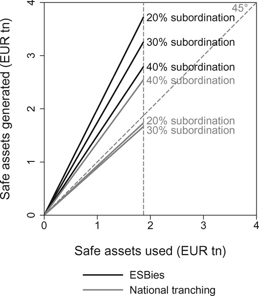
Supply of safe assets
Notes: Figure plots the volume of safe assets used in the securitization (horizontal axis) against those generated by the securitization (vertical axis). The solid lines refer to fixed subordination levels of ; those in black refer to ESBies, while the solid grey lines refer to tranched national bonds. Solid lines above the 45° line imply net generation of safe assets; lines below it imply net destruction of safe assets. The dashed vertical grey line intercepts the horizontal axis at €1.9tn, which represents the total outstanding face value of safe central government debt securities in 2015.
In our base case of 30% subordination, ESBies have an internal multiplier of 1.74. This contrasts with national tranching, which can cause a net destruction of safe assets because the subordinated component of safe nation-states’ debt may be rendered unsafe. Only at 40% subordination does the senior bond of an additional nation-state (namely France) become safe. This explains the non-monotonicity of the multiplier as a function of the uniform subordination level.
To prevent the net destruction of safe assets by tranching already safe nation-states’ debt, one could ‘optimize’ national tranching by minimizing the subordination level per country, such that each nation-state’s senior bond has an expected loss rate just below the 0.5% threshold. For Germany, this minimum is 0%; for France, 40%; and for Italy, 77%. Overall, optimized national tranching generates a multiplier of 1.75, similar to that of ESBies with 30% subordination. The design of ESBies, however, could also be optimized so that its expected loss rate is just below 0.5%: this occurs at a subordination level of 16%, at which ESBies have an internal multiplier of 2.1 – significantly higher than that under optimal national tranching. Moreover, ESBies are more robust to parameter uncertainty than nationally tranched bonds, since for the latter a smaller-than-expected recovery from a default would result in a haircut for the supposedly safe senior bond.
4.3.3. The attractiveness of EJBies
One might worry that the safety of ESBies comes at the expense of very risky EJBies that no investor would want to buy. This worry is fundamentally misguided: if investors hold sovereign bonds, then they will also hold synthetic securities backed by these bonds.
In fact, EJBies will be attractive to investors seeking to leverage their exposure to sovereign risk more cheaply than by using on-balance sheet leverage. This is because the first-loss piece comes with embedded leverage, the advantage of which can be illustrated with a simple example. Take the case of a hedge fund seeking exposure to a diversified portfolio of sovereign bonds. Imagine that the hedge fund wishes to enhance its return using leverage. It has two options. It could buy a pool of sovereign bonds on margin; the prime broker would set the cost of this margin funding at the interest rate of the hedge fund’s external funding. Alternatively, the hedge fund could buy EJBies, in which leverage is already embedded. In this case, the leverage is implicitly financed at the safe interest rate of ESBies, rather than at the hedge fund’s marginal rate of external funding, which is likely to be much higher. The hedge fund can, therefore, lever its portfolio more cheaply by using the leverage embedded in EJBies.
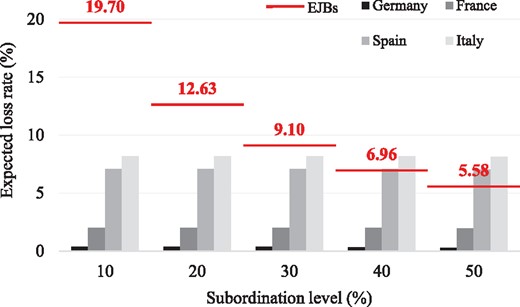
Junior bonds’ five-year expected loss rates by subordination level
Notes: Figure shows the expected loss rates of the junior tranche of national sovereign bonds versus that of the pooled euro area security. The data presented in this figure correspond to those reported in Table 4.
Junior bonds’ five-year expected loss rates in the benchmark calibration (%)
| Subordination | 10% | 20% | 30% | 40% | 50% | 60% | 70% | 80% | 90% | |
|---|---|---|---|---|---|---|---|---|---|---|
| Germany | 0.36 | 0.36 | 0.36 | 0.34 | 0.27 | 0.22 | 0.19 | 0.17 | 0.15 | |
| The Netherlands | 0.73 | 0.73 | 0.73 | 0.67 | 0.54 | 0.45 | 0.38 | 0.34 | 0.30 | |
| Luxembourg | 0.72 | 0.72 | 0.72 | 0.67 | 0.54 | 0.45 | 0.38 | 0.33 | 0.30 | |
| Austria | 1.22 | 1.22 | 1.22 | 1.17 | 1.00 | 0.84 | 0.72 | 0.63 | 0.56 | |
| Finland | 1.22 | 1.22 | 1.22 | 1.17 | 1.00 | 0.84 | 0.72 | 0.63 | 0.56 | |
| France | 1.99 | 1.99 | 1.99 | 1.98 | 1.94 | 1.81 | 1.55 | 1.36 | 1.21 | |
| Belgium | 2.52 | 2.52 | 2.52 | 2.50 | 2.49 | 2.30 | 2.02 | 1.77 | 1.57 | |
| Estonia | 3.02 | 3.02 | 3.02 | 3.01 | 3.00 | 2.85 | 2.62 | 2.29 | 2.03 | |
| Slovakia | 3.29 | 3.29 | 3.29 | 3.29 | 3.27 | 3.16 | 2.93 | 2.57 | 2.28 | |
| Ireland | 3.53 | 3.53 | 3.53 | 3.53 | 3.51 | 3.50 | 3.26 | 2.97 | 2.64 | |
| Latvia | 5.21 | 5.21 | 5.21 | 5.19 | 5.16 | 5.13 | 4.72 | 4.28 | 3.80 | |
| Lithuania | 5.19 | 5.19 | 5.19 | 5.17 | 5.14 | 5.11 | 4.70 | 4.26 | 3.79 | |
| Malta | 5.76 | 5.76 | 5.76 | 5.75 | 5.70 | 5.66 | 5.31 | 4.90 | 4.36 | |
| Slovenia | 7.07 | 7.07 | 7.07 | 7.07 | 7.02 | 6.98 | 6.60 | 6.12 | 5.44 | |
| Spain | 7.07 | 7.07 | 7.07 | 7.07 | 7.02 | 6.98 | 6.61 | 6.12 | 5.44 | |
| Italy | 8.18 | 8.18 | 8.18 | 8.18 | 8.12 | 8.07 | 7.62 | 7.04 | 6.25 | |
| Portugal | 13.03 | 13.03 | 13.03 | 13.03 | 12.78 | 12.53 | 12.13 | 11.01 | 9.96 | |
| Cyprus | 21.11 | 21.11 | 21.11 | 21.11 | 20.26 | 19.26 | 18.55 | 16.66 | 15.09 | |
| Greece | 55.39 | 55.39 | 55.39 | 55.39 | 53.85 | 48.99 | 45.51 | 41.89 | 37.72 | |
| EJBies | 19.70 | 12.63 | 9.10 | 6.96 | 5.58 | 4.65 | 3.99 | 3.49 | 3.10 | |
Notes: Table shows the junior bonds’ five-year expected loss rates (in percentage) in the benchmark calibration described in Subsection 4.3. It corresponds to the summary data presented in Figure 8. The first row of the table refers to the subordination level, which defines the size of the junior bond. The remaining rows refer to the bonds of nation-states and, in the final row, EJBies (i.e. the junior tranche of the pooled security). Numbers in black denote five-year expected loss rates below 7%, which represents the approximate threshold below which bonds would be rated investment grade, while numbers in grey denote expected loss rates above this threshold.
One might wonder whether markets have sufficient capacity to absorb a large quantity of EJBies with risk characteristics similar to those of the four lowest-rated euro area nation-states. With an underlying portfolio of €1tn, for example, EJBies with 30% subordination would have a face value of €0.3tn. At the same time, they would supplant €0.21tn of Italian, Portuguese, Cypriot and Greek debt, and an additional €0.11tn of Spanish debt, so that the overall supply of such moderately risky securities would not change much. Moreover, a hypothetical €0.3tn market for EJBies should be compared with the global high-yield market: non-euro area nation-states rated BB or BBB had outstanding debt of €4.1tn in 2012. EJBies would appeal to investors in such high-yield securities, as they would deliver high expected returns owing to their embedded leverage.
4.3.4. Sub-tranching EJBies to cater to different investors
In principle, the EJB component could be sub-tranched or repackaged in ways that make them more desirable to investors with different risk appetites. For instance, it is possible to sub-tranche the junior bond into a first-loss ‘equity’ piece and a mezzanine bond, each catering to a different clientele, as envisaged by Corsetti et al. (2016). Risk-averse investors, such as insurance companies and pension funds, would be attracted to the mezzanine bond; others specialized in high-yield debt, such as hedge funds, would prefer the first-loss piece.
We consider three sub-tranching types: a 50/50 split, whereby the equity piece comprises 15%, and the mezzanine bond 15%, of the underlying face value; a two-thirds/one-third split, whereby the equity piece comprises 20% and the mezzanine bond 10%; and a third case in which the equity piece comprises 25% and the mezzanine bond 5%.
With the 50/50 split, the mezzanine bond has an expected loss rate of 2.68%. This is slightly lower than that of Latvian sovereign bonds and slightly higher than Irish sovereign bonds, and maps to a credit rating of approximately A (i.e. ranked 6 on a 1–22 rating scale), which is firmly investment grade. The equity piece has an expected loss rate of 15.52%, which is slightly higher than that of Cypriot sovereign bonds, and would be assigned a credit rating of B+ (i.e. ranked 14 on a 1–22 rating scale), making it a ‘speculative’ high-yield security.
As the size of the equity piece increases, such that the mezzanine bond is protected by a larger first-loss piece, the expected loss rate of the mezzanine bond falls. With a 10% mezzanine bond and a 20% equity piece, the expected loss rate of the mezzanine falls to 2.40%, which is similar to that of Irish sovereign bonds and maps to a credit rating of approximately A+ (i.e. ranked 5 on a 1–22 rating scale). With a 5% mezzanine bond and a 25% equity piece, the expected loss rate of the mezzanine falls to 1.54%, which is similar to that of Belgian bonds and maps to a rating of AA (i.e. ranked 3 on a 1–22 rating scale).
Similarly, the expected loss rate of the equity piece decreases as its size increases, since the same quantum of losses is spread over a larger tranche. With a 5%/25% split between mezzanine and equity, the equity piece has an expected loss rate of 10.61%, which is slightly below that of Portuguese sovereign bonds and below investment grade. At this level of riskiness, the equity piece would be an attractive investment proposition for hedge funds and other specialized investors in high-yield debt.
4.4. Adverse calibration of the numerical simulation
In the benchmark calibration of the simulation, commonality in defaults comes from credit ratings conditional on the aggregate state, namely whether the euro area economy is in the catastrophic state 1, bad state 2 or good state 3. To consider a more adverse calibration, we build in further cross-country dependence. This provides a pessimistic robustness check and allows us to evaluate how ESBies would perform in adverse conditions relative to other security designs. We make four additional contagion assumptions, imposed sequentially in the following order:
Whenever there is a German default, others default with 50% probability.
Whenever there is a French default, other nation-states default with 40% probability, except the five highest rated nation-states, which default with 10% probability.
Whenever there is an Italian default, the five highest rated nation-states default with 5% probability; the next three nation-states (France, Belgium and Estonia) default with 10% probability; and the other nation-states default with 40% probability – unless any of these nation-states had defaulted at step 1 or 2.
Whenever there is a Spanish default, the five highest rated nation-states default with 5% probability; the next three nation-states default with 10% probability; and the other nation-states default with 40% probability – unless any of these nation-states had defaulted at step 1, 2 or 3.6
These contagion assumptions substantially increase cross-country default correlations, as is evident in Panel B (relative to Panel A) of Table 2. The first principal component of defaults now explains 42% of covariation in default rates, compared with 29% in the benchmark calibration, and the first three principal components account for 64% of the covariation compared with 57% before. Table 5 shows the conditional default probabilities, which given the way we calibrated the adverse simulation have the feature that euro area nation-states are very sensitive to the default of Germany, France, Italy or Spain.
Conditional default probabilities (%)
| Benchmark calibration | Adverse calibration | |||||||
|---|---|---|---|---|---|---|---|---|
| conditional on a default by: | conditional on a default by: | |||||||
| Germany | France | Spain | Italy | Germany | France | Spain | Italy | |
| Germany | 100 | 3 | 2 | 2 | 100 | 18 | 12 | 11 |
| The Netherlands | 7 | 6 | 4 | 4 | 26 | 19 | 14 | 14 |
| Luxembourg | 7 | 6 | 4 | 4 | 25 | 20 | 14 | 14 |
| Austria | 10 | 9 | 7 | 7 | 28 | 22 | 16 | 16 |
| Finland | 10 | 9 | 7 | 7 | 28 | 22 | 16 | 16 |
| France | 17 | 100 | 11 | 11 | 46 | 100 | 28 | 27 |
| Belgium | 20 | 19 | 14 | 13 | 44 | 45 | 31 | 30 |
| Estonia | 24 | 22 | 16 | 16 | 46 | 47 | 32 | 32 |
| Slovakia | 24 | 23 | 17 | 16 | 70 | 69 | 62 | 61 |
| Ireland | 28 | 25 | 19 | 18 | 70 | 70 | 63 | 62 |
| Latvia | 35 | 33 | 25 | 24 | 72 | 72 | 65 | 64 |
| Lithuania | 35 | 33 | 25 | 24 | 72 | 72 | 65 | 64 |
| Malta | 39 | 36 | 28 | 27 | 73 | 73 | 66 | 65 |
| Slovenia | 44 | 41 | 32 | 31 | 75 | 74 | 68 | 67 |
| Spain | 43 | 40 | 100 | 31 | 81 | 77 | 100 | 67 |
| Italy | 47 | 44 | 35 | 100 | 84 | 79 | 72 | 100 |
| Portugal | 56 | 52 | 44 | 43 | 80 | 79 | 74 | 73 |
| Cyprus | 62 | 59 | 52 | 51 | 82 | 82 | 77 | 77 |
| Greece | 88 | 86 | 82 | 81 | 93 | 93 | 91 | 91 |
Notes: Table shows the default probabilities of euro area nation-states (given in the rows of the table) conditional on the default of Germany, France, Spain or Italy (given in the columns). These conditional default probabilities are shown for the benchmark calibration (Subsection 4.3) and the adverse calibration (Subsection 4.4). In the benchmark calibration, correlations between nation-states’ default probabilities arise entirely out of the state of the euro area economy and similarity in credit ratings. Default probabilities are otherwise independent. Conditional default probabilities are shown for the benchmark calibration for comparison with those of the adverse calibration, in which there are four additional contagion assumptions governing the correlation matrix of default probabilities. Owing to these additional contagion assumptions, default probabilities conditional on the default of Germany, France, Spain or Italy increase monotonically in the adverse calibration relative to the benchmark calibration of the simulation model. If Italy defaults, for example, Spain then has a probability of default of 67% in the adverse calibration, up from 31% in the benchmark calibration. This underscores the severity of the adverse calibration of the simulation model.
Five-year expected loss rates for status quo sovereign bonds are much higher than in the benchmark calibration (Table 6). Now, only untranched German sovereign bonds are safe, so that status quo safe asset supply is €1.1tn, compared with €1.9tn in the benchmark calibration. France’s expected loss rate increases from 1.09% in the benchmark to 1.94% in the adverse calibration; Spain’s from 4.90% to 6.80%; and Italy’s from 5.63% to 7.22%.
Five-year expected loss rates in the adverse calibration (%)
| Subordination | 0% | 10% | 20% | 30% | 40% | 50% | |||||
|---|---|---|---|---|---|---|---|---|---|---|---|
| Tranche | S | J | S | J | S | J | S | J | S | J | |
| Germany | 0.50 | 0.40 | 1.43 | 0.27 | 1.43 | 0.11 | 1.42 | 0.00 | 1.26 | 0.00 | 1.01 |
| The Netherlands | 0.69 | 0.55 | 1.94 | 0.38 | 1.94 | 0.16 | 1.93 | 0.00 | 1.73 | 0.00 | 1.38 |
| Luxembourg | 0.69 | 0.55 | 1.94 | 0.38 | 1.94 | 0.16 | 1.93 | 0.00 | 1.73 | 0.00 | 1.38 |
| Austria | 0.96 | 0.80 | 2.41 | 0.60 | 2.41 | 0.35 | 2.40 | 0.09 | 2.27 | 0.00 | 1.93 |
| Finland | 0.96 | 0.80 | 2.41 | 0.60 | 2.41 | 0.35 | 2.40 | 0.09 | 2.27 | 0.00 | 1.93 |
| France | 1.94 | 1.75 | 3.66 | 1.51 | 3.66 | 1.20 | 3.66 | 0.81 | 3.63 | 0.33 | 3.54 |
| Belgium | 2.64 | 2.40 | 4.80 | 2.10 | 4.80 | 1.71 | 4.80 | 1.22 | 4.76 | 0.54 | 4.74 |
| Estonia | 3.10 | 2.87 | 5.23 | 2.57 | 5.23 | 2.19 | 5.23 | 1.70 | 5.20 | 1.03 | 5.18 |
| Slovakia | 5.58 | 5.16 | 9.30 | 4.65 | 9.30 | 3.98 | 9.30 | 3.13 | 9.25 | 1.97 | 9.19 |
| Ireland | 6.05 | 5.68 | 9.40 | 5.21 | 9.40 | 4.62 | 9.40 | 3.83 | 9.37 | 2.80 | 9.30 |
| Latvia | 6.81 | 6.38 | 10.66 | 5.85 | 10.66 | 5.16 | 10.66 | 4.26 | 10.62 | 3.09 | 10.53 |
| Lithuania | 6.80 | 6.37 | 10.64 | 5.84 | 10.64 | 5.15 | 10.64 | 4.26 | 10.61 | 3.08 | 10.52 |
| Malta | 7.32 | 6.91 | 11.04 | 6.39 | 11.04 | 5.73 | 11.04 | 4.85 | 11.03 | 3.72 | 10.92 |
| Slovenia | 8.17 | 7.74 | 12.05 | 7.20 | 12.05 | 6.51 | 12.05 | 5.59 | 12.05 | 4.41 | 11.94 |
| Spain | 6.80 | 6.45 | 9.94 | 6.02 | 9.94 | 5.46 | 9.94 | 4.71 | 9.94 | 3.75 | 9.86 |
| Italy | 7.22 | 6.85 | 10.58 | 6.38 | 10.58 | 5.78 | 10.58 | 4.98 | 10.58 | 3.96 | 10.49 |
| Portugal | 11.80 | 11.21 | 17.12 | 10.47 | 17.12 | 9.52 | 17.12 | 8.25 | 17.12 | 6.78 | 16.82 |
| Cyprus | 16.07 | 15.12 | 24.61 | 13.93 | 24.61 | 12.41 | 24.61 | 10.37 | 24.61 | 8.41 | 23.73 |
| Greece | 35.19 | 32.79 | 56.77 | 29.79 | 56.77 | 25.94 | 56.77 | 20.80 | 56.77 | 15.15 | 55.23 |
| Pooled | 3.84 | ||||||||||
| ESBies/EJBies | 2.02 | 20.24 | 1.02 | 15.13 | 0.42 | 11.81 | 0.15 | 9.38 | 0.03 | 7.64 | |
Notes: Table shows the five-year expected loss rates (in percentage) in the adverse calibration described in Subsection 4.4. The first row refers to the subordination level, which defines the size of the junior bond. The second row refers to the tranche type; ‘S’ (in black) denotes the senior bond and ‘J’ (in grey) the junior bond. The cell referring to 0% subordination is blank, since there is no tranching in this case: all bonds are pari passu. The remaining rows refer to the bonds of nation-states and, in the final row, the pooled security, which represents a GDP-weighted securitization of the 19 euro area nation-states’ sovereign bonds.
Only pooling or only tranching does not increase safe asset supply. The expected loss rate of the pooled security rises from 2.79% in the benchmark calibration to 3.84%: pure pooling, therefore, generates no safe assets. With national tranching, the five highest rated nation-states’ senior bonds are safe with 30% subordination, so the internal multiplier is 1.1. One must increase the subordination level to 50% for French senior bonds to qualify, at which point the internal multiplier is 1.45.
Again, ESBies make a significant difference. In our base case of 30% subordination, the expected loss rate is 0.42%, compared with 0.09% in the benchmark calibration. Therefore, even in this adverse calibration of our simulation model, ESBies are slightly safer than German bunds. Moreover, at 2.48, ESBies’ internal multiplier is even higher in the adverse than in the benchmark calibration.
ESBies’ safety is ensured by the junior bond, which naturally is riskier in the adverse calibration than in the benchmark one. With 30% subordination, EJBies’ five-year expected loss rate is 11.81%, compared with 9.10% in the benchmark calibration. Nevertheless, EJBies could still be sub-tranched to create an investment grade 15%-thick mezzanine bond with an expected loss rate of 6.38%, protected by a 15%-thick equity piece with an expected loss rate of 17.24%.
5. A MODEL OF THE DIABOLIC LOOP
The simulations presented in the previous section are based on fixed estimates of sovereign default probabilities and correlations. Probabilities, however, would change if euro area banks were to reduce the home bias of their sovereign portfolios, either by holding a diversified portfolio of bonds or by holding ESBies. Since there is no historical case of such portfolio rebalancing, we turn to theoretical analysis to understand how default probabilities and their correlations would change with different compositions of banks’ sovereign portfolios.
The structure of banks’ sovereign portfolios affects sovereign default probabilities for the reasons described in Section 2. Insofar as banks hold fewer domestic sovereign bonds, home-grown sovereign risk is less likely to destabilize them, which in turn mitigates concerns about sovereigns’ solvency. However, if banks hold more foreign sovereign bonds, they become more exposed to the solvency risk of foreign sovereigns, so that shocks may spread across borders via the balance sheets of banks.
We analyse these issues through the lens of a model of the diabolic loop. Brunnermeier et al. (2016) focus on the polar cases in which banks hold only domestic sovereign debt, an equally weighted portfolio of domestic and foreign sovereign debt, or ESBies. We extend their model to a continuum of portfolios, spanning the entire spectrum from complete home bias to complete diversification, either via pure pooling or pooling-cum-tranching (ESBies). This extension is important from a policy perspective because future prudential regulation is unlikely to induce complete diversification, even if it reduces the extent of banks’ home bias.
Our analysis uncovers three main results. First, without tranching, international diversification of banks’ sovereign portfolios can be a blessing (if banks are well capitalized) or a curse (if they are weakly capitalized). Second, ESBies reduce the number of states in which contagion can occur and expand those in which no diabolic loop can occur. Third, the extent to which ESBies have this effect depends on their design: greater subordination enhances the safety of ESBies, as shown numerically in Section 4, and therefore reduces the number of states in which the diabolic loop can occur.
5.1. The model
Here, we present the layout of the model and its main results graphically, and leave the detailed presentation of assumptions and derivations to the Web Appendix.
In the model, there are two countries, each populated by four agents: (i) the government, which prefers higher to lower output, as this is associated with greater tax revenue; (ii) dispersed depositors, who run on insolvent banks if the government does not bail them out, and also pay taxes; (iii) bank equity holders, who hold all of their wealth in initial bank equity, so that they cannot recapitalize banks subsequently; and (iv) investors in government bonds, whose beliefs determine the price of sovereign debt.7 The two countries are identical, so there is no loss of generality in focusing the analysis only on one of them, which we shall refer to as the domestic country.
Initially, there is a unit-size outstanding supply of zero-coupon domestic sovereign bonds with face value . Domestic banks are endowed with a sovereign bond portfolio that may include domestic sovereign bonds, a pooled security (comprising domestic and foreign sovereign bonds in equal weights), or some combination of both. We express banks’ holdings of domestic sovereign bonds as a fraction α of the total face value , so that the face value of banks’ domestic holdings is . Likewise, we express banks’ holdings of the pooled security as a fraction β of , so that the face value of banks’ holdings of the pooled security is .8 The total face value of banks’ overall sovereign portfolio is then . Note that β can be interpreted as an indicator of the extent to which banks’ portfolios are diversified. Beside sovereign debt securities, banks’ assets include loans L0 to the real economy. Their liabilities are formed by deposits D0 and equity. The market value of equity depends on the market price of sovereign debt.
Now consider the case in which the pooled security is tranched. Banks hold some portion of the senior bond (ESBies), while the junior bond (EJBies) is held exclusively by non-bank investors.9 In this case, we still denote the face value of banks’ holdings of ESBies by . Hence, the total face value of banks’ overall sovereign portfolio remains . Note that face value of ESBies is obtained by tranching face value of the pooled security, where f is one minus the subordination level.
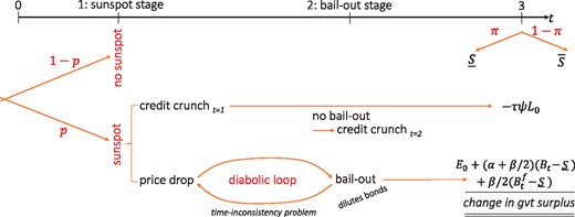
Model timeline
Notes: At t = 1, a sunspot occurs with probability p independently in each country. If it occurs, sovereign bonds fall in value; when the price drop is sufficiently large, banks cannot roll over their lending to the real economy. At t = 2, the government decides whether to bail out the banks. At t = 3, the government’s surplus is revealed. The pay-off to bondholders is the size of that surplus minus any reduction in tax revenue (owing to the credit crunch) at t = 1 and the cost of the bail-out (if it took place) at t = 2.
At t = 1, a sunspot – i.e. a confidence crisis – occurs with probability p independently in each country. This sunspot carries no fundamental information, and can be interpreted as the random variable that governs whether each nation-state defaults in each draw of the simulation in Section 4. If the sunspot occurs, non-bank investors become pessimistic about the government’s ability to repay its obligations at t = 3. This causes the price of government bonds at t = 1, B1, to drop, reducing the marked-to-market value of banks’ equity. If this repricing renders the market value of banks’ equity negative, banks cannot roll-over maturing loans of size , leading to an equal output loss that reduces the government’s revenue by at t = 3. Hence, investors’ pessimism can by itself generate a credit crunch that weakens the government’s fiscal position.
At t = 2, if a sunspot occurred at t = 1, the government decides whether to bail out banks before discovering its tax revenue at t = 3. If it does not, insolvent banks are unable to roll-over a further of maturing loans, resulting in a deeper credit crunch and even lower tax revenues at t = 3. If instead the government bails out the banks, it must issue additional government bonds, which are given to the banks as extra assets.
Finally, at date t = 3, the government’s fiscal surplus is realized, and all consumption takes place. If no sunspot occurred, the surplus is just the stochastic variable S, which is low () with probability and high () with probability. If a sunspot occurred at t = 1 and a bail-out occurred at t = 2, the surplus is equal to S, minus the tax loss due to the credit crunch at t = 1, minus the cost of recapitalizing the banks (i.e. ). For example, in the case in which banks hold only domestic bonds (β = 0), they are in need of recapitalization if the reduction in the value of their bonds, , is greater than their equity at t = 0, , or equivalently if their equity at t = 1, , is negative. The probability that the government defaults at t = 3 is the probability that the fiscal surplus is lower than .
5.2. The diabolic loop in equilibrium
In the absence of pooling or tranching, and under suitable parameter restrictions, there are two possible equilibria. If investors do not expect the government to bail out domestic banks, they also expect that the government will repay , even with a low realization of the surplus. As a result, banks will not suffer a capital loss. But if banks’ initial equity is sufficiently low, a second equilibrium – the diabolic loop – can arise. Investors expect the government to bail out banks, eroding the value of government bonds at t = 1. This triggers the need for bank recapitalization, which – in tandem with the recessionary effect of the attendant credit crunch – validates investors’ initial bail-out expectation, leading to a sovereign default when . The sunspot picks this bad equilibrium with probability p. A time-inconsistency problem is at the root of this bad equilibrium: if the government could credibly commit to never bail out banks, the diabolic loop would not arise.
Importantly, the diabolic loop equilibrium can occur if the fraction of domestic sovereign debt held by banks exceeds a threshold value relative to banks’ equity. In this case, if investors become pessimistic due to the sunspot, the sovereign debt repricing will make banks insolvent, prompting the government to bail them out, which in turn precipitates sovereign default and justifies the investors’ pessimism. Policy-makers can reduce the probability of a diabolic loop, or even exclude it entirely, by increasing bank equity requirements and reducing the fraction of domestic sovereign bonds that banks are permitted to hold. If banks are not well capitalized, however, reducing the fraction of domestic sovereign bonds held by banks and increasing the fraction of β of the pooled security held by banks increases their vulnerability to a foreign sunspot.
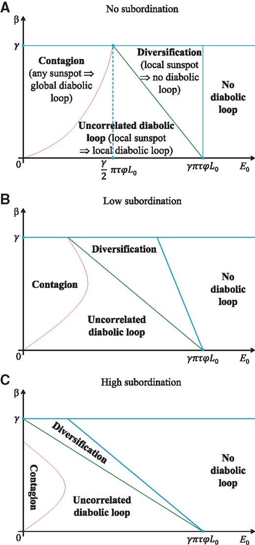
Diabolic loop regions by ESBies’ subordination level
Notes: Figure analyses the case in which there is tranching at no (Panel A), low (Panel B) and high (Panel C) levels of subordination. As subordination increases, the no diabolic loop region increases, while the other regions shrink. In the limit, when subordination is very high, the contagion and diversification regions disappear.
Consider first the case of no tranching, shown in Panel A of Figure 10. When E0 exceeds the critical value , banks are so well capitalized that the diabolic loop cannot occur, even if banks’ sovereign debt portfolios are composed entirely of domestic debt (i.e. β = 0), and regardless of the subordination level. In this case, a sovereign bond sell-off would be unjustified even following a global sunspot, because banks’ initial equity is so large that the government could recapitalize them without defaulting. Hence, in equilibrium no bond repricing would occur at date t = 1.
For values of E0 below (but not too low), if banks hold a well-diversified portfolio of sovereign debt (i.e. with sufficiently high β), a local sunspot – that is, a loss of confidence in the solvency of the home country only – cannot trigger the diabolic loop. In this diversification region, the repricing of banks’ sovereign portfolios following a local sunspot is so limited that they do not become insolvent. The benefits of diversification, however, are absent in the event of a global sunspot, when a simultaneous diabolic loop in both countries can still occur, although only with probability p2.
For even lower values of E0 or lower levels of diversification β, there exists the uncorrelated diabolic loop region, in which diversification is too limited to bring either benefit or harm. In this region, a country-specific sunspot will trigger the diabolic loop only in the country concerned. Hence, the probability of a diabolic loop occurring in the domestic country being triggered is simply that of a sunspot occurring there, i.e. p.
For even lower E0 or higher β, one enters the contagion region, in which diversification turns from a blessing into a curse. Here, a country-specific sunspot triggers a global diabolic loop: given banks’ weak capitalization and diversified portfolios, a sunspot in either country brings down the banks and sovereigns in both countries. In this region, from the perspective of each country, the probability of the diabolic loop being triggered, i.e. , is larger than in the region with uncorrelated diabolic loops, where the probability is p. In the spirit of Wagner (2010), full diversification (without tranching) by individual institutions can facilitate contagion across countries. The policy lesson is that simply increasing banks’ diversification (without ESBies) may be harmful rather than beneficial if they are poorly capitalized, as it will increase contagion.
5.3. ESBies: shift to a new equilibrium
If banks were instead to use ESBies to diversify their sovereign portfolios, the contagion region would endogenously shrink compared to the case of no tranching, and the region in which no diabolic loop can occur would expand at the expense of the diversification region. Figure 10 shows that the magnitude of these endogenous changes increases as a function of ESBies’ subordination level. With a higher subordination level, the potential for a local sunspot triggering a global crisis decreases, and so does its ability to trigger a local crisis. The intuition for this result is that tranching shifts default risks to junior bond holders outside of the banking sector. Tranching is thus a positive sum game, as it reduces the endogenous risk of a diabolic loop. In fact, if subordination were very high, both the contagion and the diversification regions would vanish. Of course, as we know from the simulations in Section 4, choosing a very high degree of subordination also reduces the supply of ESBies, so it does not come as a free lunch.
The model also sheds light on how to design the shift to a new equilibrium in a way that does not entail unintended side effects. To see this, imagine that the status quo is characterized by very low bank equity (E0) and extreme home bias (β = 0). Without ESBies, the economy may feature uncorrelated diabolic loops: a domestic sunspot triggers a domestic diabolic loop, but not a global one. If policy-makers were to design ESBies with a low subordination level, and banks were to replace the entirety of their sovereign bond portfolios with ESBies (so that ), the new equilibrium would be characterized by contagion, in which a domestic sunspot in either country triggers a global diabolic loop, insofar as E0 remains very low. This insight carries two policy implications. First, ensure that ESBies are designed with an adequate subordination level, such that they are truly safe; and second, impose stringent equity requirements on banks as a complement to the creation of ESBies.
The key insight of the model is that the probability of sovereign defaults and their cross-country correlation are both affected by the structure of banks’ balance sheets. Specifically, the probability of default depends on bank capitalization; the diversification of banks’ sovereign portfolios; and whether diversification takes place with or without tranching. The diabolic loop equilibrium can be avoided if banks are adequately capitalized. At lower levels of bank equity, the possibility of a diabolic loop equilibrium can still be avoided if banks hold ESBies. Without tranching, diversification can increase the probability of a diabolic loop by facilitating cross-country contagion. Accordingly, by introducing ESBies and incentivizing banks to hold them, policy-makers would lower the probability of sovereign defaults and reduce their cross-country correlation.
6. LAYING THE GROUNDWORK FOR ESBIES
Sovereign Bond-Backed Securities (SBBSs) are novel assets. In this section, we describe how to lay the groundwork for their creation. We address five questions: (i) How would SBBSs integrate with banking regulation? (ii) To what standards should their issuance adhere? (iii) Who would issue SBBSs? (iv) How would they interact with sovereign bond issuance? (v) How would sovereign debt restructuring change in the presence of SBBSs?
6.1. Future reform of banking regulation
Breaking the diabolic loop between sovereign risk and bank risk is a major aim of regulatory reform in Europe (Juncker et al., 2015). To date, policy-makers have pursued this objective by improving the resilience of banks and sovereigns in isolation. Banks are subject to tighter capital requirements and resolution rules, and sovereigns have improved their fiscal balance and acquired access to emergency lending facilities. These measures weaken the diabolic loop, but are not sufficient because they do not diversify banks’ sovereign bond portfolios.
6.1.1. Status quo in EU banking regulation
Banking regulation facilitates home bias in banks’ sovereign bond portfolios by setting risk weights on exposures to central governments at zero and by exempting them from large exposure limits (European Systemic Risk Board, 2015).10 As a result, euro area banks may hold sovereign bonds without funding them with any equity (as long as the leverage ratio requirement does not bind). This is logically inconsistent with the Lisbon Treaty’s ‘no-bail-out’ clause, which is founded on the premise that government debt securities are risky, and in certain states of the world might be defaulted upon. The absence of any capital charge incentivizes banks to hold risky sovereign bonds rather than other assets of similar riskiness. This manifests as home bias, particularly when sovereign risk increases: politicians encourage banks to buy domestic sovereign bonds, and banks’ sovereign bond holdings allow them to collectively correlate their risks (Farhi and Tirole, 2016).
6.1.2. SBBSs as the complement to regulatory reform
If these regulations are so damaging, why not assign capital charges to sovereign debt? Without SBBSs, such reforms could have unintended consequences. SBBSs, therefore, enable the smooth implementation of regulatory reform.
To see this, imagine that capital charges were set as a function of risk. Banks would prefer to satisfy liquidity requirements by holding low-risk sovereign debt. Without SBBSs, this could generate a regulatory-driven flight to safety from vulnerable to less-vulnerable nation-states. SBBSs preclude this outcome, as banks could satisfy liquidity requirements by holding zero risk-weighted ESBies, backed by all nation-states’ bonds.
Another argument against risk-based capital charges rests on their procyclicality. Raising the risk weight on sovereign debt in a crisis might lead banks to sell bonds, thereby lowering their price. With a union-wide safe asset there would be no such fire sales: ESBies’ safety ensures that their risk weight would not increase at times of crisis, and banks would not suffer capital losses when their sovereign encounters difficulties.
Rather than set capital charges as a function of risk, regulators could set them according to banks’ concentration in individual sovereign issuers. Banks would be incentivized to diversify their portfolios, avoiding a regulatory-driven flight to safety. But there are two drawbacks. First, banks would hold a diversified portfolio without the seniority offered by tranching. Our analyses in Sections 4 and 5 revealed that such a portfolio would not be safe; diversification without tranching can even facilitate cross-border contagion.
The second drawback of concentration-based capital charges is that they might incentivize only partial diversification. In the euro area, the four largest nation-states account for more than four-fifths of outstanding sovereign debt securities. With a portfolio comprised of these four nation-states’ debt securities, the marginal diversification benefit would be minimal. Small frictions in banks’ ability to operate in other sovereign bond markets might, therefore, dissuade them from full diversification. Consequently, smaller nation-states with relatively illiquid sovereign bond markets could be penalized by concentration-based capital charges. ESBies solve this conundrum, as they represent a fully diversified and liquid security that banks could buy with minimal transaction costs.
6.1.3. Risk weights on ESBies and EJBies
As part of regulatory reform, policy-makers should define the treatment of ESBies and EJBies. Under current regulation, they would both be treated as securitizations, and would, therefore, attract a harsh treatment relative to that of sovereign debt. This de facto penalization – which extends across the regulatory landscape, from banks and insurers to other financial institutions – explains SBBSs' current non-existence.
To reflect ESBies’ relative safety, and to encourage their issuance, policy-makers should carve out SBBSs' regulatory treatment by defining them as quasi-sovereign debt. EJBies, instead, are risky securities and should be treated as such. If they were not, banks would be able to arbitrage regulation (by holding EJBies rather than ESBies or sovereign bonds) and the diabolic loop would partly remain. Take a bank holding a replicating portfolio with a share f of ESBies and a share of EJBies, where is the subordination level. If the weighted-average risk weight of directly held sovereign bonds were X%, and since ESBies’ risk weight is fixed at zero, EJBies’ risk weight must be , so that . Importantly, this ‘look-through principle’ takes into account the tranching structure embedded in the asset-backed security. Similar considerations apply to the regulation of insurers and other financial institutions.
6.2. The SBBS Handbook
Besides regulation, another impediment to the creation of a market for SBBSs is coordination failure, which inhibits issuance by multiple private-sector entities. To address these problems, public institutions should play a standard-setting and certification role. An official SBBS Handbook should set out the key characteristics to which issuers must adhere when designing the securities, including their subordination level, the portfolio weights, and the allocation of the arbitrage margin. A security created by an authorized SBBS issuer according to these guidelines would then be awarded a ‘license number’ that certifies it as a legitimate SBBS. This process of SBBS certification would ensure that different issues of SBBSs are homogeneous, and therefore liquid, transparent and trusted by investors, who understand that the securities do not entail any explicit or implicit joint liability.
6.2.1. Subordination level
As we highlight in Section 4, the choice of the subordination level embeds a trade-off between ESBies’ safety and size. Our base case subordination level is 30%, at which ESBies would be as safe as German bunds. The Handbook should set this level so that it is the same across different issues of SBBSs. This is a transparent and objective characteristic of the securitization.
6.2.2. Portfolio weights and price discovery
To reflect SBBSs' status as union-wide assets, portfolio weights should be set according to nation-states’ relative contributions to the euro area economy. This is strictly better than setting weights according to nation-states’ outstanding public debt, which would embed a severe moral hazard problem: by issuing more debt, countries could increase their share in the securitization. In general, weight recalculations should be infrequent to preserve a high degree of homogeneity among outstanding SBBSs. This could be done by calculating a moving average of countries’ relative GDPs with a window of, say, five years; similarly, one could assign weights in proportion to national central banks’ shares in the ECB’s capital, which is slow-moving by design.
One problem with the GDP weighting is that several nation-states in the euro area have little public debt outstanding relative to their GDP. As of 2015, the nation-state with the lowest ratio of central government debt to GDP was Estonia (at 0%), followed by Luxembourg (12%), Latvia (25%), and Lithuania (34%), as shown in Table 1. A simple solution would be to modify the portfolio weights if SBBSs include all of a nation-state’s outstanding bonds, with weights on the remaining elements scaled up proportionally.
The problem with this simple re-weighting scheme is that SBBS issuers would buy all of the outstanding debt of certain nation-states, so that ordinary price discovery could no longer take place. But reliable price discovery is a cornerstone of SBBSs. To maintain price discovery, the SBBS Handbook could adopt the rule followed by the ECB in its public sector purchase programme, so that the underlying pool would include only up to k% of a nation-state’s outstanding bonds, with the SBBS issuer purchasing these bonds at the market price of the % still traded on secondary markets. When the k% constraint binds, the weights on the remaining elements of the portfolio would be scaled up proportionally so that the weights sum to 100%.
With this k% rule, a large market for ESBies and EJBies – in excess of approximately €1.5tn in total – would require either significant portfolio re-weighting in favour of countries with larger debt stocks (which is undesirable) or parameterization of k% above the 33% used in the Eurosystem’s public sector purchase programme (which might distort price discovery). Instead, issuers could be permitted a small amount of discretionary ‘wiggle-room’ in their choice of portfolio weights – for example, by underweighting one country and overweighting the two ‘neighboring’ countries in terms of credit rating, so that the overall risk of the portfolio stays the same. With multiple private-sector SBBS issuers, such wiggle-room would strengthen the process of price discovery on primary markets. An overpriced sovereign bond, for example, would be underweighted by competitive SBBS issuers, which seek to assemble SBBS-eligible portfolios at the lowest price. Such primary market price discovery could permit a higher parameterization of k%, so that the market for ESBies and EJBies could grow to be very large in steady state.
6.2.3. Exclusion of certain nation-states
SBBSs require price discovery of national sovereign bonds. When a country loses primary market access, its bonds should not be included in new issues of SBBSs. We call this the ‘market access criterion’. SBBS issuers are supposed to purchase sovereign bonds at market prices: purchases cannot happen in the absence of such prices. Moreover, the inclusion in the underlying portfolio of a country without market access would make it difficult to place EJBies, potentially giving rise to contagion. To avoid these spillover effects, newly issued SBBSs should only include central government bonds with an active secondary market, for which price discovery is ensured.
Excluding a country that loses primary market access from new issues of SBBSs has the additional advantage of strengthening fiscal discipline, as the penalty from losing market access would be larger. Hatchondo et al (2017) show a similar incentive effect in the context of bonds carrying mutual guarantees (‘Eurobonds’). In their model, the introduction of Eurobonds with a ‘default exclusion’ clause, whereby defaulting countries are not included in new Eurobond issues, lowers credit spreads in the short run because countries’ incentives for strategic default decrease.
Besides this market access criterion, the portfolio underlying SBBSs should comprise all nation-states. Otherwise, arbitrary exclusion would reduce safe asset supply. To see this, note that any exclusion entails a volume effect, by which the face value of the senior bond is reduced (holding the subordination level fixed), and a risk effect, which captures the change in the subordination level required to keep ESBies’ expected loss rate constant. The volume effect always dominates the risk effect, even for risky nation-states. Consequently, the exclusion of any nation-state unambiguously reduces the supply of safe assets for given cross-country default correlations.
For instance, compare our benchmark – in which ESBies with 30% subordination have a safe asset multiplier of 1.74 – with alternative securities that exclude Italy and, in a separate exercise, Spain. These two countries are chosen arbitrarily for their size and moderate riskiness; in unreported results, we conduct similar exercises for other countries, with qualitatively similar findings. Without Italy, ESBies’ safe asset multiplier stands at 1.45; Spain’s exclusion puts it at 1.55 (holding the subordination level constant at 30%). These reductions of 0.29 and 0.19 points (relative to the benchmark multiplier of 1.74) represent the negative volume effect. In both cases, however, the same level of safety can be achieved with a lower subordination level: 24% without Italy, and 28% without Spain. These adjustments lead to positive risk effects of 0.12 and 0.04 points, respectively, resulting in safe asset multipliers of 1.58 without Italy and 1.59 without Spain – both lower than the benchmark multiplier of 1.74 in which no country is excluded.
The key insight is that there is no trade-off between the union-wide, proportionate provision of the safe asset and maximization of the volume of safe assets, for fixed correlation structures. This is because each nation-state’s debt contains a component, however small, that with tranching can be made safe. We conclude that SBBSs should be backed by all euro area nation-states with primary market access. Only if a nation-state loses market access should it be excluded from the portfolio.
6.2.4. Liquidity premia and the excess spread
With SBBSs, national sovereign bonds might feature thinner markets and, therefore, higher liquidity premia (Foucault et al., 2013). But this drawback would be offset by the creation of highly liquid markets for ESBies and EJBies. In steady state, the liquidity premium on ESBies and EJBies would be lower than the weighted-average liquidity premia on the national sovereign bonds from which they are created. In securitizations, this wedge is called the ‘excess spread’ or ‘arbitrage margin’.
The accrual and allocation of this arbitrage margin should be defined in the SBBS’ Handbook. One possibility would be to deposit in a residual interest tranche all of the arbitrage margin accrued over the life of the securitization. If a default occurs, this residual interest tranche would cover the first loss, providing additional protection to EJBies. If no default occurs, the residual interest tranche could be paid to nation-states according to their weights in the securitization. Alternatively, a more refined disbursement arrangement would compensate nation-states in proportion to the cost that they bear in terms of higher liquidity premia following the advent of SBBSs. In this way, SBBSs could lead to a net gain in terms of the overall liquidity premium paid by each nation-state.
6.3. Who would issue SBBSs?
SBBSs can be issued by any entity. The two most likely candidates are either the securitization vehicles of private financial institutions, such as large banks or asset managers, or a public institution, such as the European Stability Mechanism. This choice is not exclusive: SBBSs could be issued by some combination of private and public entities.
6.3.1. Public versus private
Assigning responsibility for issuing SBBSs to a single public institution would ensure that the instruments have homogeneous characteristics. The SBBS’ Handbook would be fully respected, as the public institution would have no incentive to deviate from the Handbook’s specifications or engage in market manipulation. Moreover, a public institution could be depended upon for continuous issuance even during banking crises, when some private financial institutions might have their functions impaired.
A public SBBS issuer must be independent from political interference with respect to SBBS’ design. This poses a governance challenge, and perhaps requires new EU legislation. By contrast, private-sector issuance would not require any such legal change, and would exploit the fact that many such institutions have pre-existing expertise in securitizations. Importantly, competing private SBBS issuers would strengthen price discovery in the primary markets for sovereign debt. Private-sector issuers could also compete to design differently sub-tranched junior securities that are most attractive to investors, while ensuring that SBBSs are designed in accordance with the Handbook.
In the case of private issuance, a licensing body, which could be an existing public institution, would authorize prospective issuers. Licences would be given to reputable private financial institutions that fulfil some requirements defined in the Handbook, particularly in terms of the necessary financial expertise and experience. Beyond these basic requirements, it is important to ensure that the holders of ESBies and EJBies do not face counterparty risk.
6.3.2. Minimizing counterparty risk
Counterparty risk might arise due to risk of default by the issuer, legal risk, or moral hazard in forming and monitoring the portfolio of bonds.
To mitigate counterparty credit risk, SBBSs should be made bankruptcy remote from the issuer’s own balance sheet by using special purpose vehicles to hold the underlying portfolios of bonds. Thus, in case of default of the issuer, resolution procedures could extract the SBBS operations of the issuer from the rest of its activities, and carry on servicing and honoring previously issued SBBSs.
To address legal risk, the public licensing body could require SBBS issuers to operate only in jurisdictions with reliable legal frameworks. The body could even require issuance to take place in a single jurisdiction, so that all SBBSs are subject to the same laws.
Issuers of asset-backed securities are usually subject to two types of counterparty moral hazard. The first is in selecting the underlying asset pool. This risk is absent in the case of SBBSs because issuers would have no discretion with respect to asset selection. The second source of moral hazard is in monitoring the corresponding debtors and enforcing payments. Because the underlying pool is made of sovereign bonds, the collection of payments takes minimal effort. Therefore, it is not necessary to require the SBBS issuer to retain a fraction of the junior bond.
6.4. Dealing with diversity in sovereign bond markets
SBBS issuers could purchase sovereign bonds both on primary and secondary markets. Activity on secondary markets would be facilitated by European issuers’ tendency to top-up on-the-run bonds. But primary markets are characterized by cross-country heterogeneity in terms of the timing and characteristics of issues. Coordination among debt management offices (DMOs) and some ingenuity by SBBS issuers would overcome this heterogeneity.
6.4.1. Heterogeneity in the timing of issues
Heterogeneity in the timing of issues creates warehousing risk for the SBBS issuer that must hold sovereign bonds for a short period of time, subject to market and credit risk, until it assembles the complete portfolio and places the corresponding ESBies and EJBies. To some extent, warehousing risk is inevitable in any securitization activity, and is compensated by the fees and spreads that accrue to the issuer. In the case of ESBies, it is mitigated by the liquidity of the underlying sovereign bonds, easing the process of buying them in secondary markets. Moreover, issuers could sell ‘to-be-announced’ securities – whereby an issuer sells forward contracts for delivery of ESBies and EJBies on a pre-agreed date. This reduces warehousing risk by placing the ESBies and EJBies at the same time as the underlying sovereign bonds are purchased.
Warehousing risk could be significantly reduced if purchases were to happen mostly at primary issuance. This would be facilitated by coordination among DMOs, as proposed by Giovannini (2000). DMOs would have strong incentives to coordinate, since SBBS issuers would provide a large and steady demand for national bonds. While this is not necessary for ESBies to be created, it would simplify matters.
6.4.2. Heterogeneity in bond maturities
Almost all nation-states in the euro area issue plentiful one-year, five-year and ten-year nominal bonds. Still, in any one month, several nation-states might not issue anything in these maturity buckets. This problem could be partly overcome by the SBBS issuer buying sovereign bonds also in secondary markets. In addition, DMOs could reopen previous issues of 10-year bonds to help provide a supply of underlying assets. Insofar as the problem remains, SBBS issuers could engage in time tranching, on top of the credit tranching that is at the heart of ESBies. Time tranching, which is standard in the issuance of MBSs, consists of buying bonds of different maturities and then using their payouts to service synthetic securities of different maturities.
6.4.3. Heterogeneity in other bond characteristics
Euro area sovereign bonds differ in their coupons, indexing and other characteristics. Again, greater coordination among DMOs would simplify SBBS issuance. However, nation-states have different cash-flow requirements and preferences, so some degree of heterogeneity in bond characteristics is unavoidable. This need not prevent the creation of SBBSs, since issuers have the technical capability to group sovereign bonds with slightly different characteristics. They have faced and overcome greater challenges with private securities.
6.5. Governance during restructuring
SBBSs issuers hold underlying bonds. Yet, having sold all tranches, issuers have no incentive to act according to SBBS holders’ interests during a restructuring procedure.
In private-sector securitizations, a standard solution is to require the issuer to retain a fraction of the junior bond. This is not necessary, however, as transparency with respect to the underlying portfolio rules out any scope for manipulation. An alternative is to employ a special servicer that adheres to a servicing standard and maximizes value on behalf of all investors. The special servicer is typically controlled by junior investors; post-crisis arrangements include an operating advisor, appointed by the senior investors, to balance any bias that the special servicer might have in favour of junior bondholders. With SBBSs, this model would concentrate considerable power in the hands of a small number of agents, who would likely be subject to lobbying by special interests.
A better arrangement would be to apply a ‘look-through principle’ to the voting rights of ESB and EJB holders in proportion to the underlying face value of the securitization. This broad distribution of voting rights avoids concentrations of power and any bias in favour of either holding-out or restructuring.
7. CATALYSING THE MARKET FOR ESBIES
Reform of the regulatory treatment of banks’ sovereign exposures (Subsection 6.1), an ESBies’ Handbook (Subsection 6.2), the certification of SBBS issuers (Subsection 6.3) and coordination of sovereign bond issuance (Subsection 6.4) are necessary preconditions for an ESBies market. Policy intervention, however, is necessary to kickstart the market for ESBies. We envision this process taking place in three stages.
7.1. Stage one: incremental growth
At first, SBBS issuance could be limited. Regular issues of, say, €1bn per month would allow contract details to be refined. Investors could learn about ESBies’ utility as a safe store of value, and SBBS issuers could acquire information regarding the marginal cost of issuance, and to charge fees accordingly. Over time, as market participants digest the new security, the pace of regular issuance could be gradually increased.
7.2. Stage two: deepening the market for ESBies
Limited issuance is useful in the early years, but it cannot elicit the full benefits of ESBies.11 One option to enlarge the market could be to arrange for a centralized auction mechanism, whereby bank and non-banks participants submit a price schedule for sovereign bonds, ESBies and EJBies. After the auction, SBBS issuers would hold the underlying sovereign bonds, banks would have ESBies and maybe some EJBies, and non-bank investors would acquire primarily EJBies. While this auction may seem involved, it is no more complex than the spectrum auctions of telecommunications frequencies.
Following the large-scale swap, the market for ESBies would achieve critical mass, in terms of both liquidity and safe asset supply. Future policy-makers may decide to maintain market size at such a level, or continue to facilitate its growth. Further growth should not impede efficient price discovery, which is essential for market discipline.
7.3. Stage three: transition to the new regulatory regime
Once the market for ESBies attains a critical mass, the new banking regulations could be introduced gradually, allowing banks to comply within a transition period. In this transition, lower-than-adequate risk weights for national sovereign debt and EJBies would persist for a short while. Nevertheless, markets may put pressure on banks to engage in front-running, as happened with capital requirements. Banks may try to move quickly to meet the future regulatory requirements and use the swap auction to immediately satisfy the new steady state regulation. Such front-running is acceptable as long as there is a well-functioning, liquid market for ESBies to facilitate banks’ portfolio rebalancing.
7.4. The role of the European Central Bank
The ECB is a big player in sovereign debt markets. The central bank would benefit from the presence of ESBies, which provide for a union-wide safe asset with which to perform monetary policy operations, thereby simplifying risk management decisions. The ECB could catalyse the market for ESBies in two ways.
First, the ECB could announce that it would accept ESBies as collateral in monetary policy operations, as suggested by Brunnermeier et al. (2011) and Garicano and Reichlin (2014). As a general rule, banks should have no reason to hold sovereign bonds instead of ESBies. The haircut rate at which the ECB would accept ESBies as collateral in monetary policy operations should reflect ESBies’ safety, sending a powerful signal to markets.
Second, the ECB could use ESBies as its preferred security for open market operations or quantitative easing. If warranted by its price stability mandate, the ECB could purchase ESBies without bearing default risk. In the short run, with the national sovereign bonds that it already owns and following the rules in the SBBS Handbook, the ECB could facilitate market creation by selling sovereign bonds to SBBS issuers.
8. CONCLUSION
This paper makes three main contributions. First, we assess ESBies’ safety via numerical simulations. With adequate subordination, ESBies would be safe even under adverse conditions and would increase the supply of euro safe assets. Second, theoretical analysis reveals that the sovereign-bank diabolic loop can be weakened insofar as banks hold ESBies rather than home-biased sovereign debt portfolios. Third, we outline the operational steps necessary to create SBBSs. After policy-makers change regulation and set common standards, SBBS issuance should start at a small scale before being deepened.
With these three contributions, we try to advance the policy debate on ESBies. Clearly, this debate would benefit from further analysis along several dimensions, including ESBies’ risk properties under alternative scenarios; appropriate portfolio weights; and the roles of public- and private-sector entities in SBBS issuance. We hope that these further analyses will lay the groundwork for making ESBies a reality in financial markets.
Discussion
Elena Carletti
Bocconi University
The ESBies constitute a union-wide safe asset without joint liability across countries. Their aim is to ameliorate two important problems currently plaguing the euro area: (i) lack of safe assets (the Eurozone has only €2.6tn bonds of DE, NL, and LU corresponding to 25% of its GDP, while the US Treasuries amount to 105% of the US GDP); (ii) presence of a diabolic loop between sovereign and bank risk, which leads to flight towards bond issued by safe countries in times of crises.
How would ESBies ameliorate these two problems? First, ESBies would duplicate the supply of assets with a 30% junior tranche. Second, they would reduce the diabolic loop significantly since, by constituting a union-safe asset, they would entail a flight to safe assets rather than to safe countries in time of crises.
In essence, the proposal consists of the securitization of euro area government bonds. The idea is to construct a diversified portfolio of sovereign bonds and split it into a tranche composed of senior bonds (the so-called ESBies) and a junior tranche composed of junior bonds (the so-called European Junior Bonds, EJBies). The underlying portfolio should be formed by bonds of all euro area sovereigns in proportion of national GDP. Both diversification and tranching are needed to ensure the safety of the senior tranche with a junior tranche of about 30%. Given these features, ESBies appear to be a ‘win-win’ security: they are safer than the German bunds and do not entail any mutualization.
How do the authors prove the benefits of ESBies? They first perform various simulations to prove the quantitative properties of ESBies. In particular, they show that:
ESBies would be as safe as the AAA-rated bonds of DE, NL, and LU with 30% subordination;
the creation of ESBies would be adequate for banks to use them as a safe store of value as they would more than double the status quo supply of safe assets; and
there would be enough demand for EJBies given that their expected loss rate would be comparable to that of vulnerable Euro area countries.
Then, the authors build a theoretical model to show the qualitative properties of ESBies. The main result is that ESBies can ameliorate the diabolic loop between banks and sovereigns by reducing the contagion states and increasing those where no loop is present. Finally, the authors put forth a handbook with instructions as to how implement the ESBies proposal. These include suggestions on the subordination level, portfolio weights, issuers, diversity in sovereign bond issuances, transition versus steady state, governance during restructuring, etc.
This discussion will centre on the simulation exercises the authors perform and on some implementation proposals. Let me start from the former. The first comment refers to the three scenarios used to perform the simulations: severe recession, mild recession, and expansion. The data used for these scenarios are in line with the US business cycle in the period 1854–2010. Given the analysis focuses in Europe though, it would be helpful to know whether they are also consistent with the European business cycle.
The second comment refers more specifically to the granularity and correlations of the portfolio underlying ESBies. The crucial aspect in the creation of the CDOs is that the underlying assets are many and not very correlated. In the case of ESBies, by contrast, the underlying portfolio is formed by bonds issued by a limited number of different countries, which are strongly interconnected both financially and economically. This implies that the portfolio underlying the ESBies is more likely to exhibit strong correlations and that the benefit of diversification is likely more limited than in the case of CDOs. One question is how important these aspects are, in particular for the pricing of ESBies. Although the authors are very careful in calculating the correlations of the underlying portfolios, the reported numbers (see in Table 2) appear a bit low. Just to make an example, one could reasonably imagine that a German default would have much more severe effects on the other countries than shown in the table. Importantly also, correlations should take account of the effect of the feedback effects between banks and sovereigns.
A further consideration on the simulation exercises concerns the high concentration in the underlying portfolio, where German bonds account for approximately 28%, French bonds for 17%, and Italian and Spanish bonds for about 11%. How important is this, for the safety of ESBies and again for the correlations among bonds and countries? Related to this, the safety of ESBies depends crucially on the recovery rates in case of default, and it is well known, calculating recovery rates for states is much more complicated than for corporates. States are not liquidated even if in default and seizing their assets can be quite difficult. Thus, how are the recovery rates calculated and what makes them different across countries? Is it due to the fact that countries have different assets, or does it depend on factors such as the quality of the legal system or the quality of the domestic institutions?
Let me now move to the implementation side of ESBies. As explained above, the proposal is carefully crafted and it contains a large number of implementation details, which help increase both the attractiveness and the realism of the proposal. Still, the ESBies are subject to significant political sensitivity, in part because they need to reconcile the interests of many different parties: the stronger countries, which may fear ESBies as a mutualization exercise; the weaker countries, which may be asked to accept new regulatory requirements in exchange for the creation of ESBies; the debt managers, as they may perceive ESBies as a threat to the liquidity of their respective domestic sovereign bond markets and may fear that some coordination in debt issuances will be required with the creation of ESBies; the market participants as potential issuers and buyers of ESBies; and the ECB as possible initial coordinator and promoter of the ESBies issuances.
Given the numerous parties involved and their different interests and objectives, the creation of ESBies is an economic as well as a political challenge. The question is what arguments can be made to convince all the involved parties. This is a point where the authors may want to dig a bit deeper going forward. For example, the paper argues that stronger countries should appreciate that ESBies reduce the probability of crises and as well as the need for bailouts in a crisis as banks would be less exposed to sovereigns. But how attractive is this argument for the stronger countries given that, at least according to Maastricht, in principle there should just be no bailouts and weaker countries should first of all implement the necessary reforms to strengthen their economic fundamentals? And how about the weaker countries? How can they be convinced that the potential costs of ESBies in terms of new regulatory requirements are needed to improve the long-term sustainability of both the sovereign and the banking sector? Moving to debt managers, how can their debt issuances be more coordinated if countries have different needs? What do we know about the current structure of the sovereign market? How different or similar is it across countries? Finally, the market, how easily is to price ESBies and EJBies? Certainly, pricing the tranched securities seems to be more difficult than pricing the underlying assets because of the difficulty in knowing and estimating the correlations among them. Could the pricing be easier if there were more tranches? Alternatively, could it help to enlarge the underlying portfolio by including the regional and local government bonds e.g. the debt issued by municipalities?
Two final important implementation issues concern the governing law of the new securities and the inclusion of defaulted states with non-marketable debt. Most euro area sovereign debt is issued under domestic law, and particularly so for the larger countries (Germany, France, Italy, and Spain). In which law would the new securities be issued, and does the governing law of the tranched securities matter for the underlying assets? The Greek experience has indeed shown that sovereign bonds in domestic law are subject to an important commitment problem in that the government can retroactively change contracts and default mechanisms. Issuing ESBies and EJSbies under a law that ties the hands of the issuers and guarantees legal safety in time of default is crucial for the attractiveness of these securities and thus for generating sufficient market demand.
A final related issue concerns the rules for defaulted states. Would their bonds be included in the underlying portfolio even if they are no longer tradable? Including them would help keeping the representation of the portfolio, while at the same time, however, reducing the overall marketability and possibly the attractiveness of the tranched securities.
To conclude, ESBies are a simple but powerful idea. They are gaining political momentum, but for this it is important to push further their design and analyse in depth the numerous aspects they entail. In line with this, it would be helpful to run simulations under more extreme scenarios on the correlations of bonds in the underlying portfolio and to dig deeper into the calculation of the recovery rates. Further, the creation of ESBies entails implications for many actors in both the public and private sectors. Recognizing their different interests and objectives is crucial to ensure the attractiveness of ESBies and their final implementation. All in all, the ESBies proposal is simple and attractive, but politically sensitive. Still, it is certainly worth pushing it further.
Panel discussion
In response to Elena Carletti (discussant), Sam Langfield clarified that many of the comments raised regarding the simulations were already addressed to some extent in the most recent version of the paper that contains several alternative calibrations of the model e.g. scenarios with higher LGDs, higher PDs, more frequent severe recessions. Nevertheless, he acknowledged that the authors can test for the robustness of the results even further and announced that their intention is to put the simulation code online so that other researchers can themselves examine different setups. He also explained that it is difficult to have precise estimates of LGD rates given the absence of past observations on sovereign debt restructurings in Europe (i.e. most occurred in emerging markets). However, many of the alternative specifications they use were precisely designed to account for this. In terms of the political economy of the proposal and the conflicting concerns in different parts of Europe, Sam Langfield recognized that there is no easy answer but argued that ESBies may be an important step towards decreasing banks’ exposure to domestic sovereign debt, particularly in periphery countries.
Richard Portes first stated that this proposal does not deal with the debt overhang problem in Europe. He also said that only using AAA-rated debt as a safe asset may not be appropriate and can end up exaggerating the advantages of ESBies, as described by the authors. Finally, he claimed that the legal framework is a crucial issue, particularly if the United Kingdom does leave the EU. On the latter point, Sam Langfield recognized the importance of the legal framework and mentioned that the ESBies issuance should take place in the same jurisdiction in terms of insolvency law.
In their comments, Charles Bean and Richard Portes wondered why the market did not create such security in the past. Sam Langfield replied that one potential answer is that this type of securitization is very simple and, as a result, private investors may not be able to extract rents from it. George De Menil mentioned that this is indeed a very interesting proposal but still a second-best approach to correct a fundamental flaw in the construction of the euro. Sam Langfield agreed but stated that given the political constraints in relation to the first-best, ESBies may still be an excellent alternative.
Tommaso Monacelli highlighted that the paper focuses too much on the bright side of securitization, which is in contrast with what we learnt during the recent global financial crisis. He recommended the authors to do additional simulations that incorporate stronger correlated shocks and contagion effects. In a related point, Nicola Fuchs-Schündeln observed that while the simulations treat risk as completely exogenous, sovereign default probabilities can endogenously change with the introduction of ESBies.
SUPPLEMENTARY DATA
Supplementary data are available at Economic Policy online.
*This paper is prepared for Economic Policy. For insightful comments, we thank Thorsten Beck, the Economic Policy Managing Editor in charge of this paper; conference discussants, namely Elena Carletti, Mahmood Pradhan and Jeromin Zettelmeyer; members of the ESRB General Board (chaired by Mario Draghi); seminar participants at the European Central Bank and European Commission; participants at a meeting of the Fachbeirat der BaFin; participants at the 2016 annual conference on international finance at the City University of Hong Kong, and at the FRIC 2016 conference on financial frictions at Copenhagen Business School; and Iñaki Aldasoro, Spyros Alogoskoufis, Giovanni Bassani, Sascha Becker, John Berrigan, Vítor Constâncio, Daniel Dăianu, Mathias Dewatripont, Robert Düll, Peter Dunne, Tina Engler, Alberto Giovannini, Daniel Gros, Magdalena Grothe, Alexandra Hild, Andrew Karolyi, Malcolm Kemp, Neill Killeen, Philip Lane, Thilo Liebig, Davide Lombardo, Simone Manganelli, Francesco Mazzaferro, Ashoka Mody, Kitty Moloney, Mario Nava, Giulio Nicoletti, Richard Portes, Carmelo Salleo, Isabel Schnabel, Dirk Schoenmaker, Luigi Federico Signorini, Saverio Simonelli, Frank Smets, Maite de Sola Perea, Jeremy Stein, Javier Suarez, Amir Sufi, Rada Tomova, Ernst-Ludwig von Thadden, Leopold von Thadden, Jens Weidmann, Olaf Weeken, Josef Zechner and three anonymous referees. Jorge Abad, Yann Koby and Virgilijus Rutkauskas provided excellent research assistance. The views expressed herein are those of the authors and do not necessarily represent the views of the institutions to which they are affiliated.
The Managing Editor in charge of this paper was Thorsten Beck.
Other proposals are summarized by Claessens et al. (2012) and Tumpel-Gugerell (2014). Common issuance of eurobonds, contemplated by the European Commission (2011) and Ubide (2015), implies joint liability. The blue–red proposal of Von Weizsacker and Delpla (2010) entails joint liability for the first 60% of a sovereign’s debt stock (relative to GDP). The ‘eurobills’ proposal of Philippon and Hellwig (2011) involves joint issuance of short-maturity bills of up to 10% of a country’s GDP. Even the German Council of Economic Experts’ (2012) proposal for a ‘European Redemption Pact’ involves some degree of joint liability, albeit with strict conditionality, and without creating a union-wide safe asset. Hild et al. (2014) envisage a security similar to ESBies, namely a synthetic security backed by a GDP-weighted portfolio of sovereign bonds, but with partial joint liability among nation-states. To our knowledge, the only proposal for a pooled security that does not engender joint liability is that of Beck et al. (2011), whose ‘synthetic eurobond’ is comparable to ESBies without tranching. Our simulations in Section 4 and our model in Section 5 show that tranching is critical to ESBies’ safety.
We define sovereign bonds with reference to central government debt securities. The portfolio, however, could in principle comprise a broader category of public debt, such as general government debt.
We consider only the inclusion of nation-states in the euro area. The concept of ESBies, however, could be extended to other jurisdictional units. Bauer et al. (2008), for example, propose an asset-backed securitization of emerging market debt. In this case, exchange rate risk could be managed by increasing the subordination level, using foreign exchange derivatives, or requiring nation-states to issue a fraction of their debt in a common currency.
Market discipline would be enhanced by a provision that excludes from the underlying portfolio any country that has been shut out of primary markets, as we explain in Subsection 6.2.3. This ensures that market access problems in one country do not spill over to other countries by making the issuance of EJBies more difficult.
Brunnermeier et al. (2011) moot further protection for the senior bond in the form of a state-guaranteed ‘credit enhancement’. However, as we show in Section 4, credit enhancement is unnecessary to ensure the safety of the senior bond. Thus, ESBies need not encompass any public guarantee.
These four additional contagion assumptions are applied sequentially in the order in which they are described. For example, if there is a German default at step 1, all other nation-states default with a probability of 50%. If France then defaults at step 2 – which if Germany defaults happens with 50% probability, but if Germany does not default happens with probability pd1 = 25%, pd2 = 3% or pd3 = 0.05% – the nation-states with a credit rating superior to France’s default with probability 10%, if they had not already defaulted, while those with an inferior rating default with probability 40%. After this step 2, we add the default events to those from the step 1. So if a nation-state had not defaulted after step 1, but defaults in step 2 after France’s default, then it has defaulted after steps 1 and 2 taken together.
For simplicity, we assume that all agents are risk-neutral. There is no discounting, so the risk-free interest rate is zero. Short-term deposits yield extra utility compared to long-term government debt due to their convenience value in performing transactions. This is necessary to justify the demand for bank deposits backed by sovereign debt. Otherwise, banks would not need to hold sovereign debt.
We normalize one unit of the pooled security to face value . This is only a normalization: it does not imply that the total face value of the pooled security is . For example, if only a small amount of the pooled security is created, its face value will be much smaller than that of the outstanding supply of domestic sovereign bonds.
In Subsection 6.1.3, we envisage allowing banks to hold EJBies, subject to a punitive risk weight. Our modelling assumption – that non-banks are the exclusive holders of EJBies – can be interpreted in the sense that risk weights would be so punitive that banks decide not to hold any EJBies.
See the EU Capital Requirements Regulation (articles 114, 150 and 400).
In a model of endogenous safe asset determination, He et al. (2016) show that only sufficiently large issuance of a common bond lowers the risk of the remaining fraction of debt.


