Double/debiased machine learning for difference-in-differences models

Summary

This paper provides an orthogonal extension of the semiparametric difference-in-differences estimator proposed in earlier literature. The proposed estimator enjoys the so-called Neyman orthogonality (Chernozhukov et al., 2018), and thus it allows researchers to flexibly use a rich set of machine learning methods in the first-step estimation. It is particularly useful when researchers confront a high-dimensional data set in which the number of potential control variables is larger than the sample size and the conventional nonparametric estimation methods, such as kernel and sieve estimators, do not apply. I apply this orthogonal difference-in-differences estimator to evaluate the effect of tariff reduction on corruption. The empirical results show that tariff reduction decreases corruption in large magnitude.

1. INTRODUCTION

The difference-in-differences (DiD) estimator has been used widely in empirical economics to evaluate causal effects when there exists a natural experiment with a treated group and an untreated group. By comparing the variation over time in an outcome variable between the treated group and the untreated group, the DiD estimator can be used to calculate the effect of treatment on the outcome variable. Applications of DiD include but are not limited to studies of the effects of immigration on laboru markets (Card, 1990), the effects of minimum wage law on wages (Card and Krueger, 1994), the effect of tariff liberalisation on corruption (Sequeira, 2016), the effect of household income on children’s personalities (Akee et al., 2018), and the effect of corporate tax on wages (Fuest, Peichl, and Siegloch, 2018).

The traditional linear DiD estimator depends on a parallel-trend assumption that in the absence of treatment, the difference in outcomes between treated and untreated groups remains constant over time. In many situations, however, this assumption may not hold because there are other individual characteristics that may be associated with the variations of the outcomes. The treatment may be taken as exogenous only after controlling for these characteristics. However, as noted by Meyer, Viscusi, and Durbin (1995), including control variables in the linear specification of the traditional DiD estimator imposes strong constraints on the heterogeneous effect of treatment. To address this problem, Abadie (2005) proposed the semiparametric DiD estimator. Compared to the traditional linear DiD estimator, the advantages of Abadie’s estimator are threefold. First, the characteristics are treated nonparametrically so that any estimation error caused by functional specification is avoided. Second, the effect of treatment is allowed to vary among individuals, whereas the traditional linear DiD estimator does not allow this heterogeneity. Third, the estimation framework proposed in Abadie (2005) will enable researchers to estimate how the effect of treatment varies with changes in the characteristics.

The present paper provides an orthogonal extension of Abadie’s semiparametric DiD estimator (DMLDiD hereafter).¹ Abadie’s semiparametric DiD estimator behaves well when researchers use conventional nonparametric methods, such as kernel and sieve estimators, to estimate the propensity score in the first-step estimation. As shown in the classical semiparametric estimation literature, Abadie’s DiD estimator is |$\sqrt{N}$|-consistent and asymptotically normal when kernel or sieve is used in the first-step estimation. However, according to the general theory of inference developed in Chernozhukov et al. (2018), these desirable properties may fail if researchers use a rich set of newly developed nonparametric estimation methods, the so-called machine learning (ML) methods, such as Lasso, Logit Lasso, random forests, boosting, neural network, and their hybrids, in the first-step estimation. This is especially a problem when researchers confront a high-dimensional data set in which the number of potential control variables is more than the sample size, and thus the conventional nonparametric estimation methods do not apply.

In this paper, I propose DMLDiD for three different data structures: repeated outcomes, repeated cross sections, and multilevel treatment, which are all based on the original paper by Abadie (2005), as well as on the papers on the general inference theory of ML methods by Chernozhukov et al. (2018) and Chernozhukov et al. (2019). DMLDiD will allow researchers to apply a broad set of ML methods and still obtain valid inferences. The key difference is that DMLDiD, in contrast to Abadie’s original DiD estimator, is constructed on the basis of a score function that satisfies the so-called Neyman orthogonality (Chernozhukov et al. 2018), which is an important property for obtaining valid inferences when applying ML methods. With this property, DMLDiD can overcome the bias caused by the first-step ML estimation and achieve |$\sqrt{N}$|-consistency and asymptotic normality as long as the ML estimator converges to its true value at a rate faster than N^−1/4. Figure 1 shows the Monte Carlo simulation that illustrates the negative effect of directly combining ML methods on Abadie’s estimator and the benefit of using DMLDiD. The histogram in the left panel shows that the simulated distribution of Abadie’s estimator is biased, whereas the simulated distribution of DMLDiD in the right panel is centred at the true value.

Figure 1.

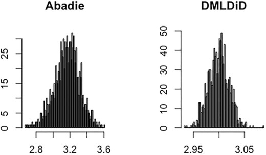
Comparison of Abadie’s DiD and DMLDiD with the first-step Logit Lasso estimation. The true value is θ₀ = 3. The results for other ML methods can be found in Section 4.

As an empirical example, I study the effect of tariff reduction on corruption by using the trade data between South Africa and Mozambique during 2006 and 2014. The source of exogenous variation is the large tariff reduction on certain commodities occurring in 2008. This natural experiment was studied previously by Sequeira (2016) using the traditional linear DiD estimator. On the basis of Sequeira’s linear specification, I include the interaction terms between the treatment and a vector of control variables. After controlling for the interaction terms, I find that the traditional linear DiD estimate becomes insignificantly different from zero. This suggests the existence of heterogeneous treatment effects, and Sequeira’s result can be interpreted as a weighted average of these heterogeneous effects. As pointed out by Abadie (2005), it is ideal to treat the control variables nonparametrically when there exists heterogeneity in treatment effects, to avoid any inconsistency caused by functional form misspecification. I apply both Abadie’s semiparametric DiD and DMLDiD on the same data set (Table 9 of Sequeira, 2016). In comparison with Sequeira’s result, though with the same sign, Abadie’s estimator is at least twice as large as previously reported by Sequeira (2016). This large effect, however, may be due to the lack of robustness of this estimation method and the finite-sample bias in the first-step nonparametric estimation. DMLDiD removes the first-order bias and suggests a smaller effect that is closer to Sequeira’s estimate. The value becomes only 60% higher than Sequeira’s result. This extra effect can be explained by the misspecification of the traditional linear DiD estimator. Therefore, I obtain the same conclusion as Sequeira (2016) that tariff reduction decreases corruption, but my estimate suggests an even larger magnitude.

The DMLDiD proposed in the present paper relies heavily on the recent high-dimensional and ML literature: Belloni et al. (2012), Belloni, Chernozhukov, and Hansen (2014), Chernozhukov et al. (2015), Belloni et al. (2017), and Chernozhukov et al. (2018). The present paper is also closely related to the robustness of average treatment effect estimation discussed in Robins and Rotnitzky (1995) and the general discussion in Chernozhukov et al. (2019). The asymptotic properties of the robust estimators discussed in those papers remain unaffected if only one of the first-step estimation with classical nonparametric method is inconsistent. In independent and contemporaneous works, Zimmert (2019), Sant’Anna and Zhao (2019), Li (2019), and Lu, Nie, and Wager (2019) also considered the orthogonal property of Abadie’s DiD estimator. Zimmert (2019) further discussed its efficiency, whereas Sant’Anna and Zhao (2019) and Li (2019) focused on classical first-step estimation. Lu, Nie, and Wager (2019) discussed the situation in which control variables are correlated with time.

1.1. Plan of the paper

Section 2 reviews both the traditional linear DiD estimator and Abadie’s semiparametric DiD estimator and discusses their limitations. Section 3 presents DMLDiD and discusses its theoretical properties. Section 4 conducts the Monte Carlo simulation to shed some light on the finite-sample performance of the proposed DiD estimator. Section 5 provides the empirical application, and Section 6 concludes the paper.

2. THE SEMIPARAMETRIC DID ESTIMATOR

In this section, I review the traditional linear DiD estimator and Abadie’s semiparametric DiD estimator. Let Y_i(t) be the outcome of interest for individual i at time t and D_i(t) ∈ {0, 1} the treatment status. The population is observed in a pre-treatment period, t = 0, and in a post-treatment period, t = 1. With potential outcome notations (Rubin, 1974), we have |$Y_{i}\left(t\right)=Y_{i}^{0}\left(t\right)+\left(Y_{i}^{1}\left(t\right)-Y_{i}^{0}\left(t\right)\right)D_{i}\left(t\right)$|⁠, where |$Y_{i}^{0}\left(t\right)$| is the outcome that individual i would attain at time t in the absence of the treatment, and |$Y_{i}^{1}\left(t\right)$| represents the outcome that individual i would attain at time t if exposed to the treatment. Because individuals are exposed to treatment only at t = 1, we have D_i(0) = 0 for all i. To reduce notation, I define D_i ≡ D_i(1). Then, the specification for the traditional linear DiD without control variables is

$$\begin{eqnarray} Y_{i}\left(t\right)=\mu +\tau \cdot D_{i}+\delta \cdot t+\alpha \cdot D_{i}\left(t\right)+\varepsilon _{i}\left(t\right), \end{eqnarray}$$

where α is the parameter of interest, ε_i(t) is an exogenous shock that has mean zero, and (μ, τ, δ) are constant parameters. If the common trend assumption holds unconditionally, then the parameter α captures the effect of treatment. When the treated and untreated groups are thought to be unbalanced with some characteristics, researchers often include a vector of control variables, |$X_{i}\in \mathbb {R}^{d}$|⁠, in the above linear specification:

$$\begin{eqnarray} Y_{i}\left(t\right)=\mu +X_{i}^{\prime }\pi \left(t\right)+\tau \cdot D_{i}+\delta \cdot t+\alpha \cdot D_{i}\left(t\right)+\varepsilon _{i}\left(t\right). \end{eqnarray}$$

As noted by Meyer, Viscusi, and Durbin (1995), including control variables in this linear specification may not be appropriate if the treatment has different effects for different groups in the population. One may also need to include the interaction terms between X_i and D_i(t) to capture the heterogeneous effect of treatment. Hence, it is ideal to treat the control variables nonparametrically, as suggested by Abadie (2005). In the following, I review Abadie’s semiparametric DiD estimator.

Let the parameter of interest be the average treatment effect on the treated (ATT):

$$\begin{eqnarray} \theta _{0}\equiv E\left[Y_{i}^{1}\left(1\right)-Y_{i}^{0}\left(1\right)\mid D_{i}=1\right]. \end{eqnarray}$$

Abadie (2005) discussed three data types: repeated outcomes, repeated cross sections, and multilevel treatment. To avoid repetition, I focus only on the first two cases. The discussion for multilevel treatments is provided in the appendix.

2.1. Case 1 (repeated outcomes)

Suppose that researchers observe both pre-treatment and post-treatment outcomes for the individual of interest. That is, researchers observe |$\left\lbrace Y_{i}\left(0\right),Y_{i}\left(1\right),D_{i},X_{i}\right\rbrace _{i=1}^{N}$|⁠. In this case, we can identify the ATT under the following assumptions (Abadie, 2005):

 

Assumption 2.1.

|$E\left[Y_{i}^{0}\left(1\right)-Y_{i}^{0}\left(0\right)\mid X_{i},D_{i}=1\right]=E\left[Y_{i}^{0}\left(1\right)-Y_{i}^{0}\left(0\right)\mid X_{i},D_{i}=0\right]$|⁠.

 

Assumption 2.2.

P(D_i = 1) > 0 and P(D_i = 1∣X_i) < 1, with probability one.

Assumption 2.1 is the conditional parallel-trend assumption. It states that conditional on the individual’s characteristics, X_i, the average outcomes for treated and untreated groups would have followed parallel paths in the absence of treatment. Assumption 2.2 states that the support of the propensity score of the treated group is a subset of the support for the untreated. With these two assumptions, Abadie (2005) identified the ATT:

$$\begin{eqnarray} \theta _{0}=E\left[\frac{Y_{i}\left(1\right)-Y_{i}\left(0\right)}{P\left(D_{i}=1\right)}\frac{D_{i}-P\left(D_{i}=1\mid X_{i}\right)}{1-P\left(D_{i}=1\mid X_{i}\right)}\right]. \end{eqnarray}$$

(2.1)

2.2. Case 2 (repeated cross sections)

Suppose what researchers observe is repeated cross-sectional data. That is, researchers observe |$\left\lbrace Y_{i},D_{i},T_{i},X_{i}\right\rbrace _{i=1}^{N}$|⁠, where Y_i = Y_i(0) + T_i(Y_i(1) − Y_i(0)), and T_i is a time indicator that takes value one if the observation belongs to the post-treatment sample.

 

Assumption 2.3.

Conditional on T = 0, the data are independent and identically distributed from the distribution of (Y(0), D, X), and conditional on T = 1, the data are independent and identically distributed from the distribution of (Y(1), D, X).

Supposing Assumptions 2.1 through 2.3 hold, the ATT is identified (Abadie, 2005) as

$$\begin{eqnarray} \theta _{0}=E\left[\frac{T_{i}-\lambda _{0}}{\lambda _{0}\left(1-\lambda _{0}\right)}\frac{Y_{i}}{P\left(D_{i}=1\right)}\frac{D_{i}-P\left(D_{i}=1\mid X_{i}\right)}{1-P\left(D_{i}=1\mid X_{i}\right)}\right], \end{eqnarray}$$

(2.2)

where λ₀ ≡ P(T_i = 1).

Then, the semiparametric DiD estimator would be the sample analog of (2.1) and (2.2). For example, in Case 1, in which researchers confront repeated outcomes data, the sample analog of (2.1) is

$$\begin{eqnarray} \hat{\theta }=\frac{1}{N}\sum _{i=1}^{N}\frac{Y_{i}\left(1\right)-Y_{i}\left(0\right)}{\hat{p}}\frac{D_{i}-\hat{g}\left(X_{i}\right)}{1-\hat{g}\left(X_{i}\right)}, \end{eqnarray}$$

where |$\hat{p}$| is the estimator of p₀ ≡ P(D = 1), and |$\hat{g}(X_{i})$| is the estimator of the propensity score g₀(X) ≡ P(D = 1∣X). When |$\hat{g}$| is estimated by using classical nonparametric methods, such as the kernel or series estimators, the estimator |$\hat{\theta }$| is able to achieve |$\sqrt{N}$|-consistency and asymptotic normality under certain conditions, as shown in the semiparametric estimation literature (Newey, 1994; Newey and McFadden, 1994).

When |$\hat{g}$| is an ML estimator, however, the estimator |$\hat{\theta }$| is not necessarily |$\sqrt{N}$|-consistent in general. According to the general theory of inference of ML methods developed in Chernozhukov et al. (2018), the reason is twofold. First, the score function based on (2.1), |$\varphi \left(W,\theta _{0},p_{0},g_{0}\right)\equiv \frac{Y\left(1\right)-Y\left(0\right)}{P\left(D=1\right)}\frac{D-g_{0}\left(X\right)}{1-g_{0}\left(X\right)}-\theta _{0}$|⁠, has a non-zero directional (Gateaux) derivative with respect to the propensity score g₀:

$$\begin{eqnarray} \partial _{g} E\left[\varphi \left(W,\theta _{0},p_{0},g_{0}\right)\right]\left[g-g_{0}\right]\ne 0, \end{eqnarray}$$

where the directional (Gateaux) derivative is defined in Section 3. Second, ML estimators usually have a convergence rate slower than N^−1/2 because of regularisation bias. Similarly, the estimators obtained by directly plugging ML estimators into (2.2) will not be |$\sqrt{N}$|-consistent in general. The Monte Carlo simulation in Section 4 supports this theoretical insight and reveals significant bias on the estimators based on (2.1) and (2.2) when ML estimators are used in the first-step nonparametric estimation.

The next section proposes DMLDiD based on (2.1) and (2.2). A distinctive feature of DMLDiD is that the Gateaux derivatives of the score functions are zero with respect to their infinite-dimensional nuisance parameters. This property helps us remove the first-order bias of the first-step ML estimation.

3. THE DMLDID ESTIMATOR

In this section, I propose DMLDiD on the basis of Abadie’s results (2.1) and (2.2). In Section 3.1, I present the new score functions derived from (2.1) and (2.2) and propose an algorithm to construct DMLDiD. In Section 3.2, I show the theoretical properties of the proposed estimator.

3.1. The Neyman-orthogonal score

Suppose Assumptions 2.1 through 2.3 hold, and consider the following new score functions.

Case 1 (repeated outcomes): The new score function for repeated outcomes is

$$\begin{eqnarray} \psi _{1}\left(W,\theta _{0},p_{0},\eta _{10}\right) & = &\frac{Y\left(1\right)-Y\left(0\right)}{P\left(D=1\right)}\frac{D-P\left(D=1\mid X\right)}{1-P\left(D=1\mid X\right)}-\theta _{0} \\ & - & \underbrace{\frac{D-P\left(D=1\mid X\right)}{P\left(D=1\right)\left(1-P\left(D=1\mid X\right)\right)}E\left[Y\left(1\right)-Y\left(0\right)\mid X,D=0\right]}_{c_{1}} \\ \end{eqnarray}$$

(3.1)

with the unknown constant p₀ = P(D = 1) and the infinite-dimensional nuisance parameter

$$\begin{eqnarray} \eta _{10}=\left(P\left(D=1\mid X\right),E\left[Y\left(1\right)-Y\left(0\right)\mid X,D=0\right]\right)\equiv \left(g_{0},\ell _{10}\right). \end{eqnarray}$$

Case 2 (repeated cross sections): The new score function for repeated cross sections is

$$\begin{eqnarray} \psi _{2}\left(W,\theta _{0},p_{0},\lambda _{0},\eta _{20}\right)=\frac{T-\lambda _{0}}{\lambda _{0}\left(1-\lambda _{0}\right)}\frac{Y}{P\left(D=1\right)}\frac{D-P\left(D=1\mid X\right)}{1-P\left(D=1\mid X\right)}-\theta _{0}-c_{2}, \end{eqnarray}$$

(3.2)

where the adjustment term c₂ is

$$\begin{eqnarray} c_{2}=\frac{D-P\left(D=1\mid X\right)}{\lambda _{0}\left(1-\lambda _{0}\right)\cdot P\left(D=1\right)\cdot \left(1-P\left(D=1\mid X\right)\right)}\times E\left[\left(T-\lambda _{0}\right)Y\mid X,D=0\right]. \end{eqnarray}$$

The nuisance parameters are the unknown constants p₀ = P(D = 1) and λ₀ = P(T = 1) and the unknown function

$$\begin{eqnarray} \eta _{20}=\left(P\left(D=1\mid X\right),E\left[\left(T-\lambda \right)Y\mid X,D=0\right]\right)\equiv \left(g_{0},\ell _{20}\right). \end{eqnarray}$$

Notice that the above new functions are equal to the original score functions (2.1) and (2.2) plus the adjustment terms, (c₁, c₂), which have zero expectations. Thus, the new score functions (3.1) and (3.2) still identify the ATT in each case. The purpose of the adjustment terms is to make the Gateaux derivative of the new score functions zero with respect to infinite-dimensional nuisance parameters, which is the so-called Neyman-orthogonal property in Chernozhukov et al. (2018). I combine the new scores (3.1) and (3.2) with the cross-fitting algorithm of Chernozhukov et al. (2018) to propose DMLDiD.

 

Definition 3.1.

(a) Take a K-fold random partition|$\left(I_{k}\right)_{k=1}^{K}$|of observation indices [N] = {1, ..., N}. For simplicity, assume that each fold I_k has the same size n = N/K. For each k ∈ [K] = {1, ..., K}, define the auxiliary sample|$I_{k}^{c}\equiv \left\lbrace 1,...,N\right\rbrace \setminus I_{k}$|⁠. (b) For each k, construct the intermediate ATT estimators,

$$\begin{eqnarray} \tilde{\theta }_{k}=\frac{1}{n}\sum _{i\in I_{k}}\frac{D_{i}-\hat{g}_{k}\left(X_{i}\right)}{\hat{p}_{k}\left(1-\hat{g}_{k}\left(X_{i}\right)\right)}\times \left(Y_{i}\left(1\right)-Y_{i}\left(0\right)-\hat{\ell }_{1k}\left(X_{i}\right)\right){ (rep-outcomes) } \end{eqnarray}$$

$$\begin{eqnarray} \tilde{\theta }_{k}=\frac{1}{n}\sum _{i\in I_{k}}\frac{D_{i}-\hat{g}_{k}\left(X_{i}\right)}{\hat{p}_{k}\hat{\lambda }_{k}\left(1-\hat{\lambda }_{k}\right)\left(1-\hat{g}_{k}\left(X_{i}\right)\right)}\times \left(\left(T_{i}-\hat{\lambda }_{k}\right)Y_{i}-\hat{\ell }_{2k}\left(X_{i}\right)\right){ (rep-cross-sections)} \end{eqnarray}$$

where|$\hat{p}_{k}=\frac{1}{n}\sum _{i\in I_{k}^{c}}D_{i}$| , |$\hat{\lambda }_{k}=\frac{1}{n}\sum _{i\in I_{k}^{c}}T_{i}$|⁠, and |$\left(\hat{g}_{k},\hat{\ell }_{1k},\hat{\ell }_{2k}\right)$|are the estimators of (g₀, ℓ₁₀, ℓ₂₀) constructed by using the auxiliary sample|$I_{k}^{c}$|⁠. (c) Construct the final ATT estimator|$\tilde{\theta }=\frac{1}{K}\sum _{k=1}^{K}\tilde{\theta }_{k}.$|

The estimators |$\left(\hat{g}_{k},\hat{\ell }_{1k},\hat{\ell }_{2k}\right)$| can be constructed by using any ML methods or classical estimators, such as kernel or series estimators. For completeness, I present the Logit Lasso and Lasso estimators here.

Consider a class of approximating functions of X_i,

$$\begin{eqnarray} q_{i}\equiv \left(q_{1}\left(X_{i}\right),...,q_{p}\left(X_{i}\right)\right)^{\prime }. \end{eqnarray}$$

For example, q_i can be polynomials or B-splines. Let Λ(u) ≡ 1/(1 + exp ( − u)) be the cumulative distribution function of the standard logistic distribution. Construct the estimator of the propensity score g₀ by

$$\begin{eqnarray} \hat{g}_{k}\left(x_{i}\right)\equiv \Lambda \left(q_{i}^{\prime }\hat{\beta }_{k}\right), \end{eqnarray}$$

(3.3)

where

$$\begin{eqnarray} \hat{\beta }_{k}\equiv \arg \min _{\beta \in \mathbb {R}^{p}}\frac{1}{M}\sum _{i\in I_{k}^{c}}\left\lbrace -D_{i}(q_{i}^{\prime }\beta )+\log \left(1+\exp \left(q_{i}^{\prime }\beta \right)\right)\right\rbrace +\lambda _{k}\parallel \beta \parallel _{1} \end{eqnarray}$$

is the Logit Lasso estimator, and M = N − n is the sample size of the auxiliary sample |$I_{k}^{c}$|⁠. Next, define M_k as the sample size of |$I_{k}^{c}\cap \left\lbrace i:D_{i}=0\right\rbrace$|⁠. Construct the estimators of ℓ₁₀ and ℓ₂₀ by

$$\begin{eqnarray} \hat{\ell }_{1k}\left(x_{i}\right)\equiv q_{i}^{\prime }\hat{\beta }_{1k}, \end{eqnarray}$$

$$\begin{eqnarray} \hat{\ell }_{2k}\left(x_{i}\right)\equiv q_{i}^{\prime }\hat{\beta }_{2k}, \end{eqnarray}$$

where

$$\begin{eqnarray} \hat{\beta }_{1k}\in \arg \min _{\beta \in \mathbb {R}^{p}}\left[\frac{1}{M_{k}}\sum _{i\in I_{k}^{c}}\left(1-D_{i}\right)\left(Y_{i}\left(1\right)-Y_{i}\left(0\right)-q_{i}^{\prime }\beta \right)^{2}\right]+\frac{\lambda _{1k}}{M_{k}}\parallel \hat{\Upsilon }_{1k}\beta \parallel _{1} \end{eqnarray}$$

and

$$\begin{eqnarray} \hat{\beta }_{2k}\in \arg \min _{\beta \in \mathbb {R}^{p}}\left[\frac{1}{M_{k}}\sum _{i\in I_{k}^{c}}\left(1-D_{i}\right)\left(\left(T_{i}-\hat{\lambda }_{k}\right)Y_{i}-q_{i}^{\prime }\beta \right)^{2}\right]+\frac{\lambda _{2k}}{M_{k}}\parallel \hat{\Upsilon }_{2k}\beta \parallel _{1} \end{eqnarray}$$

are the modified Lasso estimators proposed in Belloni et al. (2012). The choices of the penalty levels and loadings |$\left(\lambda _{1k},\lambda _{2k},\hat{\Upsilon }_{1k},\hat{\Upsilon }_{2k}\right)$| suggested by Belloni et al. (2012) are provided in the appendix.

3.2. Asymptotic properties

In this section, I show the theoretical properties of the DMLDiD estimator |$\tilde{\theta }$|⁠. In particular, I will show that the estimator |$\tilde{\theta }$| can achieve |$\sqrt{N}$|-consistency and asymptotic normality as long as the first-step estimators converge at rates faster than N^−1/4. This rate of convergence can be achieved by many ML methods, including Lasso and Logit Lasso.

The critical difference between DMLDiD and Abadie’s DiD estimator is the score functions on which they are based. The new score functions (3.1) and (3.2) have the directional (or the Gateaux) derivatives equal to zero with respect to their infinite-dimensional nuisance parameters, whereas the scores based on (2.1) and (2.2) do not have this property. This property is the so-called Neyman orthogonality in Chernozhukov et al. (2018).

The definition of the Neyman-orthogonal score provided here is slightly different from the definition in Chernozhukov et al. (2018). Instead of being orthogonal against all nuisance parameters, the Neyman-orthogonal score defined here is orthogonal against only those infinite-dimensional nuisance parameters. Formally, let θ₀ ∈ Θ be the low-dimensional parameter of interest, ρ₀ be the true value of the finite-dimensional nuisance parameter ρ, and η₀ the true value of the infinite-dimensional nuisance parameter |$\eta \in \mathcal {T}$| . Suppose that W is a random element taking values in a measurable space |$\left(\mathcal {W},\mathcal {A}_{\mathcal {W}}\right)$|⁠, with probability measure P. Define the directional (or the Gateaux) derivative against the infinite-dimensional nuisance parameter |$D_{r}:\tilde{\mathcal {T}}\rightarrow \mathbb {R}$|⁠, where |$\tilde{\mathcal {T}}=\left\lbrace \eta -\eta _{0}:\eta \in \mathcal {T}\right\rbrace$|⁠,

$$\begin{eqnarray} D_{r}\left[\eta -\eta _{0}\right]\equiv \partial _{r}\left\lbrace E_{P}\left[\psi \left(W,\theta _{0},\rho _{0},\eta _{0}+r\left(\eta -\eta _{0}\right)\right)\right]\right\rbrace ,\eta \in \mathcal {T}, \end{eqnarray}$$

for all r ∈ [0, 1). For convenience, denote

$$\begin{eqnarray} \partial _{\eta }E_{P}\psi \left(W,\theta _{0},\rho _{0},\eta _{0}\right)\left[\eta -\eta _{0}\right]\equiv D_{0}\left[\eta -\eta _{0}\right],\eta \in \mathcal {T}. \end{eqnarray}$$

In addition, let |$\mathcal {T}_{N}\subset \mathcal {T}$| be a nuisance realisation set such that the estimator of η₀ takes values in this set with high probability.

 

Definition 2.

The score ψ obeys the Neyman orthogonality condition at (θ₀, ρ₀, η₀) with respect to the nuisance parameter realisation set|$\mathcal {T}_{N}\subset \mathcal {T}$|if the directional derivative map D_r[η − η₀] exists for all r ∈ [0, 1) and|$\eta \in \mathcal {T}_{N}$|and vanishes at r = 0:

$$\begin{eqnarray} \partial _{\eta }E_{P}\psi \left(W,\theta _{0},\rho _{0},\eta _{0}\right)\left[\eta -\eta _{0}\right]=0,\text{for all }\eta \in \mathcal {T}_{N}. \end{eqnarray}$$

 

Lemma 3.1.

The new score functions (3.1) and (3.2) obey the Neyman orthogonality.

The proof of this lemma can be found in the online appendix. In fact, it is also possible to derive the Neyman-orthogonal scores with respect to both finite- and infinite-dimensional nuisance parameters. However, the functional forms are much more complicated than the score functions (3.1) and (3.2), and this will make the corresponding estimator not as neat as the estimators proposed here. Because they will enjoy the same asymptotic properties, here I focus only on the estimators based on (3.1) and (3.2).

In the following, I will discuss the theoretical properties of the new estimator |$\tilde{\theta }$| when data belong to repeated outcomes and repeated cross sections. The results of multilevel treatment can be proved by using the same arguments. Let κ and C be strictly positive constants, K ≥ 2 be a fixed integer, and ε_N be a sequence of positive constants approaching zero. Denote by ∥ · ∥_{P, q} the L^q norm of some probability measure P: ∥f∥_{P, q} ≡ (∫∣f(w)∣^qdP(w))^1/q and |$\parallel f \parallel _{P,\infty } \equiv \sup _{w} \mid f\left(w\right) \mid$|⁠.

 

Assumption 3.1 (Regularity Conditions for Repeated Outcomes).

Let P be the probability law for (Y(0), Y(1), D, X). Let D = g₀(X) + U and Y(1) − Y(0) = ℓ₁₀(X) + V₁, with E_P[U∣X] = 0 and E_P[V₁∣X, D = 0] = 0. Define G_1p0 ≡ E_P[∂_pψ₁(W, θ₀, p₀, η₁₀)] and Σ₁₀ ≡ E_P[(ψ₁(W, θ₀, p₀, η₁₀) + G_1p0(D − p₀))²]. For the above definition, the following conditions hold: (a) Pr(κ ≤ g₀(X) ≤ 1 − κ) = 1; (b) ∥UV₁∥_{P, 4} ≤ C; (c) E[U²∣X] ≤ C; (d) |$E\left[V_{1}^{2}\mid X\right]\le C$|⁠; (e) Σ₁₀ > 0; and (f) given the auxiliary sample |$I_{k}^{c}$|⁠, the estimator |$\hat{\eta }_{1k}=\left(\hat{g}_{k},\hat{\ell }_{1k}\right)$| obeys the following conditions. With probability 1 − o(1), |$\parallel \hat{\eta }_{1k}-\eta _{10}\parallel _{P,2}\le \varepsilon _{N}$|⁠, |$\parallel \hat{g}_{k}-1/2\parallel _{P,\infty }\le 1/2-\kappa$|⁠, and |$\parallel \hat{g}_{k}-g_{0}\parallel _{P,2}^{2}+\parallel \hat{g}_{k}-g_{0}\parallel _{P,2}\times \parallel \hat{\ell }_{1k}-\ell _{10}\parallel _{P,2}\le \left(\varepsilon _{N}\right)^{2}$|⁠.

 

Assumption 3.2 (Regularity Conditions for Repeated Cross Sections).

Let P be the probability law for (Y, T, D, X). Let D = g₀(X) + U and (T − λ₀)Y = ℓ₂₀(X) + V₂, with E_p[U∣X] = 0 and E_p[V₂∣X, D = 0] = 0. Define G_2p0 ≡ E_P[∂_pψ₂(W, θ₀, p₀, λ₀, η₂₀)], G_2λ0 ≡ E_P[∂_λψ₂(W, θ₀, p₀, λ₀, η₂₀)], and Σ₂₀ ≡ E_P[(ψ₁(W, θ₀, p₀, η₁₀) + G_2p0(D − p₀) + G_2λ0(T − λ₀))²]. For the above definition, the following conditions hold: (a) Pr(κ ≤ g₀(X) ≤ 1 − κ) = 1; (b) ∥UV₂∥_{P, 4} ≤ C; (c) E[U²∣X] ≤ C; (d) |$E\left[V_{2}^{2}\mid X\right]\le C$|⁠; (e) E_P[Y²∣X] ≤ C; (f) ∣E_P[YU]∣ ≤ C; (g) Σ₂₀ > 0; and (h) given the auxiliary sample |$I_{k}^{c}$|⁠, the estimator |$\hat{\eta }_{2k}=\left(\hat{g}_{k},\hat{\ell }_{2k}\right)$| obeys the following conditions. With probability 1 − o(1), |$\parallel \hat{\eta }_{2k}-\eta _{20}\parallel _{P,2}\le \varepsilon _{N}$|⁠, |$\parallel \hat{g}_{k}-1/2\parallel _{P,\infty }\le 1/2-\kappa$|⁠, and |$\parallel \hat{g}_{k}-g_{0}\parallel _{P,2}^{2}+\parallel \hat{g}_{k}-g_{0}\parallel _{P,2}\times \parallel \hat{\ell }_{2k}-\ell _{20}\parallel _{P,2}\le \left(\varepsilon _{N}\right)^{2}$|⁠.

 

Theorem 3.1.

For repeated outcomes, suppose Assumptions 2.1, 2.2, and 3.1 hold. For repeated cross sections, suppose Assumptions 2.1 through 2.3 and 3.2 hold. If ε_N = o(N^−1/4), the new ATT estimator |$\tilde{\theta }$| obeys

$$\begin{eqnarray} \sqrt{N}\left(\tilde{\theta }-\theta _{0}\right)\rightarrow N\left(0,\Sigma \right) \end{eqnarray}$$

with Σ = Σ₁₀ for repeated outcomes and Σ = Σ₂₀ for repeated cross sections.

 

Theorem 3.2.

Construct the estimators of the asymptotic variances as

$$\begin{eqnarray} \hat{\Sigma }_{1}=\frac{1}{K}\sum _{k=1}^{K}\mathbb {E}_{n,k}\left[\left(\psi _{1}\left(W,\tilde{\theta },\hat{p}_{k},\hat{\eta }_{1k}\right)+\hat{G}_{1p}\left(D-\hat{p}_{k}\right)\right)^{2}\right]\qquad ({\rm repeated\, outcomes}) \end{eqnarray}$$

$$\begin{eqnarray} \hat{\Sigma }_{2}=&& \frac{1}{K}\sum _{k=1}^{K}\mathbb {E}_{n,k}\left[\left(\psi _{2}\left(W,\tilde{\theta },\hat{p}_{k},\hat{\lambda }_{k},\hat{\eta }_{2k}\right)+\hat{G}_{2p}\left(D-\hat{p}_{k}\right)+\hat{G}_{2\lambda }\left(T-\hat{\lambda }_{k}\right)\right)^{2}\right] \\ && \qquad \qquad ({\rm repeated\, cross\, sections}) \end{eqnarray}$$

where |$\mathbb {E}_{n,k}\left[f\left(W\right)\right]=n^{-1}\sum _{i\in I_{k}}f\left(W_{i}\right)$|⁠, |$\hat{G}_{1p}=\hat{G}_{2p}=-\tilde{\theta }/\hat{p}_{k}$|⁠, and |$\hat{G}_{2\lambda }$| is a consistent estimator of G_2λ0. If the assumptions of Theorem 1 hold, |$\hat{\Sigma }_{1}=\Sigma _{10}+o_{P}\left(1\right)$| and |$\hat{\Sigma }_{2}=\Sigma _{20}+o_{P}\left(1\right).$|

Theorem 3.1 shows that DMLDiD |$\tilde{\theta }$| can achieve |$\sqrt{N}$|-consistency and asymptotic normality if the first-step estimators of the infinite-dimensional nuisance parameters converge at a rate faster than N^−1/4. This rate of convergence can be achieved by many ML methods. In particular, Van de Geer (2008) and Belloni et al. (2012) provided detailed conditions for Logit Lasso and the modified Lasso estimators to satisfy this rate of convergence. Theorem 3.2 provides consistent estimators for the asymptotic variance of |$\tilde{\theta }$|⁠. The proofs of Theorem 3.1 and Theorem 3.2 can be found in the online appendix.

4. SIMULATION

In the online appendix, I conduct Monte Carlo simulations to shed some light on the finite-sample properties of the DiD estimator of Abadie (2005) and the DMLDiD estimator |$\tilde{\theta }$| in all three data structures: repeated outcomes, repeated cross sections, and multilevel treatment. For the first-step ML estimation, I generate high-dimensional data and estimate the propensity score by Logit Lasso, Support vector machine (SVM), regression tree, random forests, boosting, and neural nets. I use random forests with 500 regression trees to estimate the remaining infinite-dimensional nuisance parameters. I find that although Abadie’s DiD estimator suffers from the bias of a variety of ML methods, the DMLDiD estimator |$\tilde{\theta }$| can successfully correct the bias and is centred at the true value. Figure 2 shows the Monte Carlo simulation and the data-generating process for repeated outcomes. Other cases and details are provided in the online appendix.

Figure 2.

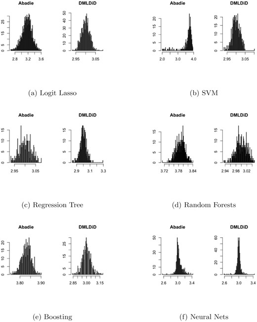
The simulation for repeated outcomes with the true value θ₀ = 3.

The data-generating process for repeated outcomes: Let N = 200 be the sample size and p = 100 the dimension of control variables, X_i ∼ N(0, I_{p × p}). Let γ₀ = (1, 1/2, 1/3, 1/4, 1/5, 0, |$...,0)\in \mathbb {R}^{p}$|⁠, and D_i is generated by the propensity score |$P(D=1\mid X)=\frac{1}{1+\exp (-X^{\prime }\gamma _{0})}.$| Also, let the potential outcomes be |$Y_{i}^{0}\left(0\right)=X_{i}^{\prime }\beta _{0}+\varepsilon _{1},$||$Y_{i}^{0}\left(1\right)=Y_{i}^{0}\left(0\right)+1+\varepsilon _{2},$| and |$Y_{i}^{1}\left(1\right)=\theta _{0}+Y_{i}^{0}\left(1\right)+\varepsilon _{3},$| where β₀ = γ₀ + 0.5 and θ₀ = 3, and all error terms follow N(0, 0.1). Researchers observe {Y_i(0), Y_i(1), D_i, X_i} for i = 1, ..., N, where |$Y_{i}\left(0\right)=Y_{i}^{0}\left(0\right)$| and |$Y_{i}\left(1\right)=Y_{i}^{0}\left(1\right)\left(1-D_{i}\right)+Y_{i}^{1}\left(1\right)D_{i}$|⁠.

5. EMPIRICAL EXAMPLE

In this example, I analyse the effect of tariff reduction on corruption behaviors by using the bribe payment data collected by Sequeira (2016) between South Africa and Mozambique. There have been theoretical and empirical debates on whether higher tariff rates increase incentives for corruption (Clotfelter, 1983; Sequeira and Djankov, 2014) or lower tariffs encourage agents to pay higher bribes through an income effect (Feinstein, 1991; Slemrod and Yitzhaki, 2002). The former argues that an increase in the tariff rate makes it more profitable to evade taxes on the margin, whereas the latter asserts that an increased tariff rate makes the taxpayers less wealthy, and this, under the decreasing risk aversion of being penalised, tends to reduce evasion (Allingham and Sandmo, 1972).

Sequeira (2016) collected primary data on the bribe payments between the ports in Mozambique and South Africa from 2007 to 2013. In exchange for tariff evasion, the cargo owners bribed the border officials who were in charge of validating clearance documentation and collecting all tariff payments. The exogenous variation used in Sequeira (2016) to study the effect of tariff reduction on corruption was the significant reduction in the average nominal tariff rate (of 5 percent) on certain products occurring in 2008. Because not all products were on the tariff reduction list, a credible control group of products is available. This credible control group allows for a DiD estimation. Sequeira (2016) pooled together the cross-section data between 2007 and 2013 and estimated the effect of treatment through the traditional linear DiD with many control variables. Table 9 of Sequeira (2016) presented the result of the following specification:

$$\begin{eqnarray} y_{it} & = &\gamma _{1}TariffChangeCategory_{i}\times POST \\ & + &\mu POST+\beta _{1}TariffChangeCategory_{i} \\ & + & \beta _{2}BaselineTariff{i}+ \Gamma _{i}+p_{i}+w_{t}+\delta _{i}+\epsilon _{it}, \end{eqnarray}$$

(5.1)

where y_it is the natural log of the amount of bribe paid for shipment i in period t, conditional on paying a bribe. TariffChangeCategory ∈ {0, 1} denotes the treatment status of commodities, POST ∈ {0, 1} is an indicator for the years following 2008, and BaselineTariff is the tariff rate before the tariff reduction. The specification also includes a vector of characteristics Γ_i, and time and individual fixed effects p_i, w_t, and δ_i. The parameter γ₁ is the parameter of interest in Equation (5.1). Sequeira (2016) found that the amount of bribe paid dropped after the tariff reduction (⁠|$\hat{\gamma }_{1}=-2.928^{**}$|⁠). However, as noted by Meyer et al. (1995), this result of Equation (5.1) excludes the heterogeneous treatment effects. The estimate might be different if we take into account the heterogeneity. To shed some light on the heterogeneous treatment effect, I incorporate the interaction terms between TariffChangeCategory × POST (TP) and the characteristics Γ_i into (5.1). The specification becomes

$$\begin{eqnarray} y_{it}& = &\gamma _{1}TariffChangeCategory_{i}\times POST+\gamma _{2}TP_{i}\times \Gamma _{i} \\ & + &\mu POST+\beta _{1}TariffChangeCategory_{i} \\ & + &\beta _{2}BaselineTariff{i}+ \Gamma _{i}+p_{i}+w_{t}+\delta _{i}+\epsilon _{it}, \end{eqnarray}$$

(5.2)

where γ₂ is a 10 × 1 vector. Table 1 shows the comparison of the estimates of (5.1) and (5.2).

Table 1.

Estimation results for (5.1) and (5.2).

	Equation (5.1)	Equation (5.2)
|$\hat{\gamma }_{1}$|	−2.928**	0.934
	(0.944)	(2.690)
TP × diff		−0.986
		(0.959)
TP × agri		−1.170**
		(0.580)
TP × lvalue		−0.098
		(0.129)
TP × perishable		0.859
		(1.213)
TP × largefirm		−0.576
		(0.988)
|$TP\times day\_arri$|		−0.002
		(0.106)
TP × inspection		−0.525
		(0.911)
TP × monitor		−0.482
		(0.713)
TP × 2007tariff		0.009
		(0.048)
TP × SouthAfrica		−2.706***
		(0.912)

Column 2 of Table 1 shows that (a) after controlling for the interaction terms, the estimate for γ₁ becomes insignificantly different from zero, and (b) most of the coefficients of the interaction terms are negative. This suggests that there exists a large set of negative heterogeneous treatment effects and that Sequeira’s estimate may be a weighted average of these heterogeneous treatment effects. The negative coefficients of the interaction terms justify the sign of Sequeira’s estimate. However, it is ideal to treat the covariates nonparametrically when there exists heterogeneity in treatment effects, to avoid any potential inconsistency created by functional form misspecification (Abadie, 2005).

I estimate the ATT using both Abadie’s DiD estimator and DMLDiD. Because the data are repeated cross sections, I construct the estimators on the basis of (2.2) and (3.2), respectively. The estimators with first-step kernel estimation contain one individual characteristic (the natural log of shipment value per ton), which is the only significant and continuous control variable in Table 9 of Sequeira (2016). The estimators with first-step Lasso estimation contain a list of the covariates included in Table 9 of Sequeira (2016), which consists of the characteristics of product, shipment, firm, and border officials. I choose both the bandwidth kernel and penalty level of Lasso by 10-fold cross validations. Table 2 shows the estimation result. First, we can observe that the estimates with first-step kernel are much larger than the estimates with first-step Lasso. The reason may be that more control variables are included in the latter estimates. Second, though with the same sign, Abadie’s estimator (−8.168 or −6.432) is at least twice as large as previously reported by Sequeira (2016). This large effect, however, may be due to not only the robustness of semiparametric estimation on the functional form but also the finite-sample bias in the first-step nonparametric estimation. The DMLDiD estimator (−5.222) removes the first-order bias and suggests a smaller effect that is closer to Sequeira’s estimate. Its value is only 60% higher than Sequeira’s result. This extra effect can be explained by the misspecification of the traditional linear DiD estimator. Therefore, I obtain the same conclusion as Sequeira (2016) that tariff reduction decreases corruption, but my estimate suggests an even larger magnitude.

Table 2.

The results of semiparametric DiD estimation.

	Sequeira (2016)	Abadie (kernel)	DMLDiD (kernel)	Abadie (Lasso)	DMLDiD (Lasso)
ATT	−2.928**	−8.168**	−6.998*	−6.432**	−5.222*
	(0.944)	(3.072)	(3.752)	(2.737)	(2.647)

6. CONCLUSION

The DiD estimator survives as one of the most popular methods in the causal inference literature. A practical problem that empirical researchers face is the selection of important control variables when they confront a large number of candidate variables. Researchers may want to use ML methods to handle a rich set of control variables while taking the strength of the DiD estimator. I improve its original versions by proposing DMLDiD to allow researchers to use ML methods while still obtaining valid inferences. This additional benefit will make DiD more flexible for empirical researchers to explore a broader set of popular estimation methods and analyse more types of data sets.

Footnotes

1

The R codes can be found on my Github: https://github.com/NengChiehChang/Diff-in-Diff

SUPPORTING INFORMATION

Additional Supporting Information may be found in the online version of this article at the publisher’s website.

Online Supplement

Replication package

Notes

Co-editor Victor Chernozhukov handled this manuscript.

APPENDIX A: MORE ON ESTIMATION

Multilevel treatments: Individuals can also be exposed to different levels of treatment. Let W ∈ {0, w₁, ..., w_J} be the level of treatment, where W = 0 denotes the untreated individuals. Researchers observe |$\left\lbrace Y_{i}\left(0\right),Y_{i}\left(1\right),W_{i},X_{i}\right\rbrace _{i=1}^{N}$|⁠. For w ∈ {0, w₁, ..., w_J} and t ∈ {0, 1}, let Y^w(t) be the potential outcome for treatment level w at period t. Denote the ATT for each level of treatment w by

$$\begin{eqnarray} \theta _{0}^{w}\equiv E\left[Y^{w}\left(1\right)-Y^{0}\left(1\right)\mid W=w\right]. \end{eqnarray}$$

Suppose that Assumptions (2.1) and (2.2) hold for each w ∈ {w₁, ..., w_J}:

$$\begin{eqnarray} E\left[Y_{i}^{0}\left(1\right)-Y_{i}^{0}\left(0\right)\mid X_{i},W_{i}=w\right]=E\left[Y_{i}^{0}\left(1\right)-Y_{i}^{0}\left(0\right)\mid X_{i},W_{i}=0\right], \end{eqnarray}$$

P(W_i = w) > 0, and with probability one, P(W_i = w∣X_i) < 1. Then, we have (Abadie, 2005),

$$\begin{eqnarray} \theta _{0}^{w}=E\left[\frac{Y\left(1\right)-Y\left(0\right)}{P\left(W=w\right)}\frac{I\left(W=w\right)\cdot P\left(W=0\mid X\right)-I\left(W=0\right)\cdot P\left(W=w\mid X\right)}{P\left(W=0\mid X\right)}\right], \end{eqnarray}$$

where I( · ) is an indicator function. The Neyman-orthogonal score function for multilevel treatments is

$$\begin{eqnarray} \psi _{w}\left(W,\theta _{w0},p_{w0},\eta _{w0}\right) &= & \frac{Y(1)-Y(0)}{P\left(W=w\right)}\frac{I(W=w)P(W=0\mid X)-I(W=0) P(W=w\mid X)}{P\left(W=0\mid X\right)} \\ & - & \theta _{w0}-c_{w}. \end{eqnarray}$$

The adjustment term c_w is

$$\begin{eqnarray} c_{w}= & \left(\frac{I\left(W=w\right)\cdot P\left(W=0\mid X\right)-I\left(W=0\right)\cdot P\left(W=w\mid X\right)}{P\left(W=w\right)\cdot P\left(W=0\mid X\right)}\right)\times \\ & E\left[Y\left(1\right)-Y\left(0\right)\mid X,I\left(W=0\right)=1\right]. \end{eqnarray}$$

The nuisance parameters are the unknown constant p_w0 ≡ P(W = w) and the infinite-dimensional parameter η_w0 = (g_w0, g_z0, ℓ₃₀), where g_w0 = P(W = w∣X), g_z0 = P(W = 0∣X), and ℓ₃₀ = E[Y(1) − Y(0)∣X, I(W = 0) = 1].

Multilevel treatments algorithm:

1. Take aK-foldrandom partition|$\left(I_{k}\right)_{k=1}^{K}$|of observation indices [N] = {1, ..., N}, such that the size of each foldI_kisn = N/K. For eachk ∈ [K] = {1, ..., K}, define the auxiliary sample|$I_{k}^{c}\equiv \left\lbrace 1,...,N\right\rbrace \setminus I_{k}$|⁠.

2. For eachk ∈ [K], construct the estimator ofp₀and λ₀by|$\hat{p}_{w}=\frac{1}{n}\sum _{i\in I_{k}^{c}}D_{i}$|⁠. Also, construct the estimators ofg_w, g_z, and ℓ₃₀by using the auxiliary sample|$I_{k}^{c}$|⁠: |$\hat{g}_{wk}=\hat{g}_{w}\left(\left(W_{i}\right)_{i\in I_{k}^{c}}\right)$|⁠, |$\hat{g}_{zk}=\hat{g}_{z}\left(\left(W_{i}\right)_{i\in I_{k}^{c}}\right)$|⁠, and|$\hat{\ell }_{3k}=\hat{\ell }_{3}\left(\left(W_{i}\right)_{i\in I_{k}^{c}}\right)$|⁠.

3. For eachk, construct the intermediate ATT estimators:

   $$\begin{eqnarray} \tilde{\theta }_{wk}& =\frac{1}{n}\sum _{i\in I_{k}}\frac{I\left(W_{i}=w\right)\cdot \hat{g}_{zk}\left(X_{i}\right)-I\left(W_{i}=0\right)\cdot \hat{g}_{wk}\left(X_{i}\right)}{\hat{p}_{w}\hat{g}_{zk}\left(X_{i}\right)}\\ & \times \left(Y\left(1\right)-Y\left(0\right)-\hat{\ell }_{3k}\left(X_{i}\right)\right). \end{eqnarray}$$

4. Construct the final ATT estimators: |$\tilde{\theta }=\frac{1}{K}\sum _{k=1}^{K}\tilde{\theta }_{k}.$|

Lasso penalty. The following is suggested by Belloni et al. (2012). Let y_i denote Y_i(1) − Y_i(0) or |$\left(T_{i}-\hat{\lambda }_{k}\right)$|⁠, λ_k denote λ_1k or λ_2k, and |$\hat{\Upsilon }_{k}$| denote |$\hat{\Upsilon }_{1k}$| or |$\hat{\Upsilon }_{2k}$|⁠. For k ∈ [K], the loading |$\hat{\Upsilon }_{k}$| is a diagonal matrix with entries |$\hat{\gamma }_{kj}$|⁠, j = 1, ..., p, constructed by the following steps:

$$\begin{eqnarray} \text{Initial }\hat{\gamma }_{kj}=\sqrt{\frac{1}{M_k}\sum _{i\in I_{k}^{c}}\left(1-D_{i}\right)q_{ij}^{2}\left(y_{i}-\bar{y}_{k}\right)^{2}},\lambda _{k}=2c\sqrt{M_{k}}\Phi ^{-1}\left(1-\gamma /2p\right), \end{eqnarray}$$

$$\begin{eqnarray} \text{Refined }\hat{\gamma }_{kj}=\sqrt{\frac{1}{M_{k}}\sum _{i\in I_{k}^{c}}\left(1-D_{i}\right)q_{ij}^{2}\hat{\varepsilon }_{i}^{2}},\lambda _{k}=2c\sqrt{M_{k}}\Phi ^{-1}\left(1-\gamma /2p\right), \end{eqnarray}$$

where |$\bar{y}_{k}=M^{-1}\sum _{i\in I_{k}^{c}}y_{i}$|⁠, c > 1 and γ → 0. The empirical residual |$\hat{\varepsilon }_{i}$| is calculated by the modified Lasso estimator |$\beta _{k}^{*}$| in the previous step: |$\hat{\varepsilon }_{i}=y_{i}-q_{i}^{\prime }\beta _{k}^{*}$|⁠. Repeat the second step B > 0 times to obtain the final loading.