Combining counterfactual outcomes and ARIMA models for policy evaluation

Summary

The Rubin Causal Model (RCM) is a framework that allows to define the causal effect of an intervention as a contrast of potential outcomes. In recent years, several methods have been developed under the RCM to estimate causal effects in time series settings. None of these makes use of autoregressive integrated moving average (ARIMA) models, which are instead very common in the econometrics literature. In this paper, we propose a novel approach, named Causal-ARIMA (C-ARIMA), to define and estimate the causal effect of an intervention in observational time series settings under the RCM. We first formalise the assumptions enabling the definition, the estimation and the attribution of the effect to the intervention. We then check the validity of the proposed method with a simulation study. In the empirical application, we use C-ARIMA to assess the causal effect of a permanent price reduction on supermarket sales. The CausalArima R package provides an implementation of the proposed approach.

1. INTRODUCTION

The potential outcomes approach is a framework that allows to define the causal effect of a treatment (or ‘intervention’) as a contrast of potential outcomes, to discuss assumptions enabling to identify such causal effects from available data, as well as to develop methods for estimating causal effects under these assumptions (Rubin, 1974, 1975, 1978; Imbens and Rubin, 2015). Following Holland (1986), we refer to this framework as the Rubin Causal Model (RCM). Under the RCM, the causal effect of a treatment is defined as a contrast of potential outcomes, only one of which is observed while the others are missing and become counterfactuals once the treatment is assigned.

Having its roots in the context of randomised experiments, several methods have been developed to define and estimate causal effects under the RCM in the most diverse settings, including networks (VanderWeele, 2010; Forastiere et al., 2020; Noirjean et al., 2020), time series (Robins, 1986; Robins et al., 1999; Bojinov and Shephard, 2019) and panel data (Rambachan and Shephard, 2019; Bojinov et al., 2020).

Focusing on observational time series data, popular methods for policy evaluation under the RCM include Difference-in-Differences (DiD) and synthetic controls methods. However, both approaches require the presence of controls that did not experience the treatment and, in case of an extensive policy change impacting all units, finding untreated units is often challenging.

A different approach to assess the impact of shocks occurring on a time series is intervention analysis, introduced in Box and Tiao (1975) and Box and Tiao (1976). The effect is generally estimated by fitting an autoregressive integrated moving average (ARIMA) type model with the addition of an intervention component whose structure should capture the effect generated on the series (e.g., level shift, slope change and similar). For example, a simple model structure that is extensively used in literature is a linear regression with ARIMA errors (REG-ARIMA henceforth) and the addition of a level shift (e.g., Larcker et al., 1980; Worthington and Valadkhani, 2004; Schaffer et al., 2021). However, intervention analysis fails to define the causal estimands and to discuss the assumptions enabling the attribution of the uncovered effect to the intervention.

Closing the gap between causal inference under the RCM and intervention analysis, in this paper we propose a novel approach, Causal-ARIMA (C-ARIMA), to estimate the causal effect of an intervention in observational time series settings where no control unit is available. In particular, we discuss assumptions under the RCM to define, estimate and attribute the effect of the intervention in such settings; we then introduce the causal estimands of interest and derive a methodology to perform inference. Finally, we illustrate how the proposed approach can be conveniently applied to solve real inferential issues by estimating the causal effect of a permanent price reduction on supermarket sales. More specifically, on 4 October 2018 the branch of a supermarket chain located in Florence (Italy) introduced a new price policy that permanently lowered the price of several store brands. The main goal is estimating the effect of the new policy on the sales of those products, as well as its indirect impact on competitor brands with the same characteristics as the discounted goods. Our results suggest that store brands’ sales increased due to the permanent price discount; interestingly, we find little evidence of a detrimental effect on competitor brands, suggesting that unobserved factors may drive competitor-brand sales more than price.

The remainder of the paper is organised as follows: Section 2 surveys the literature; Section 3 presents the causal framework; Section 4 illustrates the proposed C-ARIMA approach; Section 5 reports the results of a simulation study; Section 6 describes the empirical findings; Section 7 concludes.

2. LITERATURE REVIEW

In time series settings, the identification and the estimation of causal effects using potential outcomes have been formalised in the context of randomised experiments, see, e.g., Bojinov and Shephard (2019), Rambachan and Shephard (2019) and Bojinov et al. (2020). However, observational studies pose additional challenges to the identification and estimation of causal effects: unlike randomised experiments, the assignment mechanism, i.e., the process that determines which units receive treatment and which receive control, is unknown; in addition, in the presence of a single series receiving the intervention, estimands like the ATE (average treatment effect) are not applicable, and sometimes it might be difficult to find suitable control series.

In economics, a prediction-based causal approach for time series data is Granger–Sims causality (Granger, 1969; Sims, 1972). Despite several differences with the potential outcome framework, some connections exist between the two approaches (Rambachan and Shephard, 2019). However, as shown in Lechner (2011), neither of these concepts implies the other without additional assumptions. In addition, Holland (1986) points out that a Granger-Sims cause may become a spurious association when new information is gathered and added in the predictive model.

DiD estimators (Card and Krueger, 1993; Angrist and Pischke, 2008; Anger et al., 2011) and synthetic control methods (Abadie and Gardeazabal, 2003; Abadie et al., 2010, 2015) have been used to evaluate the effect of interventions in the absence of experimental data in a wide range of fields, including economics (Billmeier and Nannicini, 2013; Botosaru and Ferman, 2019; Ben-Michael et al., 2021) and marketing (Brodersen et al., 2015; Li, 2019). Recent developments also include their combinations, as the Synthetic Difference-in-Differences (SDiD) estimator proposed in Arkhangelsky et al. (2019), and the strand of literature on heterogeneous treatment effects with staggered adoption and variation in timing (Callaway and Sant’Anna, 2021; Sun and Abraham, 2021; Athey and Imbens, 2022). In such settings the treatment time varies across units and they remain exposed to it at all times afterwards; thus, it is possible to estimate the effect of the intervention, even when all units are eventually treated by using, as a control group, the set of last-treated units or the set of not-yet-treated units.

Nevertheless, DiD estimators, synthetic control methods and their combinations usually require to observe at least one suitable control unit, which is often impractical. For example, in our application, appropriate control series could be the sales of products that are not impacted by the new policy. However, since the supermarket chain implemented an extensive price policy change addressing at least one product in each category, all products were impacted, directly or indirectly, by the intervention. In addition, all products received the intervention simultaneously, thereby precluding the adoption of the DiD estimators developed under variation in timing. Therefore, in our setting none of the methods mentioned above is applicable.

An approach overcoming these limitations is proposed by Brodersen et al. (2015), and only requires to learn the dynamics of the treated unit prior to the intervention. In particular, the authors employ Bayesian Structural Time Series models (Harvey, 1989; West and Harrison, 2006) to build a synthetic control by forecasting the counterfactual series in the absence of intervention based on a model estimated on the pre-intervention data. Borrowing the name from the associated R package, from now on we refer to their method as ‘CausalImpact’. A generalisation of this approach is proposed in Menchetti and Bojinov (2022), where the authors employ Multivariate Bayesian Structural Time Series models to assess the impact of an intervention on statistical units showing interactions with one another.

This work is most closely related to CausalImpact and to its multivariate extension in Menchetti and Bojinov (2022), since they both consider time series setups where suitable control units are absent. In the same vein as CausalImpact, our method exploits the time dynamics in the pre-intervention period to predict the series in the absence of intervention. Similarly to Menchetti and Bojinov (2022), in the application we deal with interfering units, but we handle the interference problem by considering all units to receive an active form of treatment. Furthermore, in contrast to CausalImpact and Menchetti and Bojinov (2022), our methodology is based on ARIMA models, and can be used as an alternative by researchers and practitioners in many fields that are not familiar to (or are not willing to adopt) Bayesian inference. In addition, ARIMA models have desirable properties (tractability, consistency of the estimator of model parameters), and are suited to describe a wide variety of time series generated by complex, non-stationary processes. They are also implemented in a large number of statistical software programs, which makes C-ARIMA very easy to use in practice. The associated CausalArima R package should further promote a wide adoption of the proposed approach.¹

Therefore, C-ARIMA complements the set of tools for causal inference on observational time series data: it is tailored to estimate the effect of an intervention when no control series is available and when the number of pre-treatment periods is large, since it allows to fully exploit useful information provided by the pre-intervention dynamics; it is well suited in case of a single time series as well as for a simultaneous intervention on a large number of units (policy evaluation). Conversely, by focusing on a few time points, DiD estimators and synthetic controls have a limited ability to exploit long pre-treatment periods.²

Finally, C-ARIMA also shares many features with the approach described in Box and Tiao (1976), where the authors suggest to compare, at each point in time, the observed data after an intervention with the forecasts from a model fitted to the pre-intervention period. However, oftentimes researchers are interested in a cumulative sum of point effects, e.g., Papadogeorgou et al. (2018) focus on estimating the total number of hospital readmissions due to the Hospital Readmission Reduction Program over the entire post-intervention period. Therefore, we also provide test statistics for two additional effects: the cumulative and the temporal average effect. Most importantly, we frame our estimators in the potential outcome framework, defining the effects and discussing the assumptions enabling their attribution to the intervention: both Box and Tiao (1976) and canonical intervention analysis fail to do so, and thus it is unclear whether the effect estimated with such methods might also have a causal interpretation.

3. CAUSAL FRAMEWORK

On 4 October 2018 the Florence branch of an Italian supermarket chain introduced a new price policy that permanently lowered the price of 707 store brands in several product categories; the empirical analysis focuses on the goods belonging to the ‘cookies’ category. The supermarket chain also sells competitor-brand cookies with the same characteristics (e.g., ingredients, flavour, shape) as their store brand equivalent; starting from the intervention date, these products became more expensive compared to the store brands. As the price reduction ranges from |$-5.7\%$| to |$-23.2\%$|⁠, we expect an heterogeneous effect on each product. The main goal of the analysis is then to assess the overall impact of the price policy, which is done by estimating its causal effect on the sales of both store and competitor-brand cookies.

In this section we present the notation and introduce some assumptions allowing the definition and the estimation of the causal effect, as well as its attribution to the intervention. We also discuss their validity in our empirical setting. Finally, we define the causal estimands we are interested in.

3.1. Assumptions

Let |$\operatorname{W}_{j,t} \in \lbrace 0,1\rbrace$| be a random variable describing the treatment assignment of unit |$j \in \mathcal {V} = \lbrace 1,\dots ,J\rbrace$| at time |$t \in \lbrace 1,\dots , T\rbrace$|⁠, where 1 denotes that a ‘treatment’ (or ‘intervention’) has taken place and 0 denotes control. Lower case |$\operatorname{w}_{j,t}$| denotes a realisation of |$\operatorname{W}_{j,t}$|⁠. In general, the treatment on unit j can be allocated (or not) at each time t, thereby generating a different sequence |$\operatorname{W}_{j,1:T} = ( \operatorname{W}_{j,1}, \dots , \operatorname{W}_{j,T})$| for each unit. Instead, we restrict our attention to a setting where all units are subject to a simultaneous and persistent intervention.³

 

Assumption 3.1 (Single persistent intervention).

We say that unit j received a single persistent intervention if there exists a|$t^{*}_j$|such that|$\operatorname{W}_{j,t} = 0$|for all|$t \in \lbrace 1, \dots , t^{*}_j \rbrace$|and for all|$t \in \lbrace t_j^{*} +1, \dots , T \rbrace$|the unit is either always treated, |$\operatorname{W}_{j,t} = 1$|⁠, or always assigned to control, |$\operatorname{W}_{j,t} = 0$|⁠. If the intervention happens simultaneously on all units, we denote with|$t^{*} = t^{*}_j$|the single intervention date.

Notice that, since the treatment is irreversible, |$\operatorname{W}_{j,t} = \operatorname{W}_{j,t^{\prime }}$| for all |$t,t^{\prime } \in \lbrace t^{*} +1, \dots , T \rbrace$|⁠, thus we can drop the t subscript from the treatment variable. Both the permanent price reduction on store brands and the relative price increase on competitor brands are single persistent interventions, although the treatment definition differs for the two groups. More formally, let |$\mathcal {S} = \lbrace 1, \dots , J_s \rbrace$| and |$\mathcal {C} = \lbrace 1, \dots , J_c\rbrace$| denote the subsets of store and competitor brands, respectively; these are such that |$\mathcal {V} = \mathcal {S} \cup \mathcal {C}$| and |$J = J_s + J_c$|⁠. Then, |$\operatorname{W}_{j} = 1$| for |$j \in \mathcal {S}$| indicates the ‘permanent price reduction’ of each store brand; while |$\operatorname{W}_{j} = 1$| for |$j \in \mathcal {C}$| stands for ‘relative price increase’, whose size also varies across competitor cookies as a result of the different reductions applied to store brands.

In the RCM, the sales that we would have under treatment or control are known as potential outcomes. Although in a panel study the potential outcomes of each unit generally depend on the other units’ assignment, in our empirical setting we can exclude cross-unit interactions within each group of store and competitor brands. Indeed, the cookies selected for the permanent price discount appeal to different customers, as they differ on many characteristics, such as shape, flavor and ingredients. We call this assumption temporal no-interference.⁴ As for the interactions between the two groups, we postulate that any spillover from store to competitor brands is well captured by the relative price increase (additional spillovers due to other promotional activities on store brands are ruled out), and that competitor brands are not subject to other interventions. Furthermore, we assume that the intervention has no anticipatory effects on the outcome. This is plausible when the statistical units have no knowledge of the future intervention (see also Bojinov and Shephard, 2019; Callaway and Sant’Anna, 2021; Sun and Abraham, 2021), which is also the case of our application, since the supermarket chain did not advertise the price reduction in advance.

Therefore, under the previously discussed assumptions, we can use |$\operatorname{Y}_{j,t}(\operatorname{w}_j)$| to denote the potential outcomes time series of unit j at time t. Indeed, unit j’s potential outcomes depend solely on its assignment |$\operatorname{w}_j$|⁠. In addition, recall that there are only two potential paths for each unit in the post-intervention period, i.e., |$\operatorname{w}_j = 1$| or |$\operatorname{w}_j = 0$|⁠. These give rise to the same number of potential outcomes, but we can only observe one of them for each unit. In our case, the observed potential outcome series is |$\operatorname{Y}_{j,t}(1)$| for all units and all |$t\in \lbrace t^{*}+1, \dots , T \rbrace$|⁠, whereas |$\operatorname{Y}_{j,t}(0)$| is the missing or counterfactual potential outcome time series which is unobserved and needs to be estimated.

Including covariates that are linked to the outcome can improve the estimation of |$\operatorname{Y}_{j,t}(0)$|⁠, but if the covariates are influenced by the treatment the estimates will be biased. We therefore make the following assumption.

 

Assumption 3.2 (Covariates-treatment independence).

Let|$\operatorname{X}_{j,t}$|be a vector of covariates that are predictive of the outcome of unit j; for all|$t \in \lbrace t^{*}+1,\dots ,T \rbrace$|such covariates are not affected by the intervention, i.e., |$\operatorname{X}_{j,t}(1) = \operatorname{X}_{j,t}(0)$|⁠.

As a result, we can use the known covariates values to improve the prediction of the outcome in the absence of intervention |$\operatorname{Y}_{j,t}(0)$|⁠. As detailed in Section 6, the set of covariates in the application includes a holiday dummy, some day-of-the-week dummies and the price per unit. While it is quite obvious that all the dummies are unaffected by the intervention, things get trickier for price. For the analysis on competitor brands we used their actual price, since it is not directly affected by the intervention (only their relative price is altered by the policy); conversely, for the analysis on store brands, we assumed that the price would not have changed without the intervention.⁵

Finally, following Antonelli and Beck (2020), we use the next assumption for identification of the treatment effect.

 

Assumption 3.3 (Conditional stationarity).

Let|$\mathcal {I}_{0}$|denote the information set up to time|$t = 0$|and define|$\mathcal {I}_{t} = \lbrace \mathcal {I}_{0}, \operatorname{X}_{j,1}, \dots , \operatorname{X}_{j,t}, \operatorname{Y}_{j,1}, \dots , \operatorname{Y}_{j,t} \rbrace$|⁠, where covariates|$\operatorname{X}_{j,t}$|satisfy Assumption3.2. Indicating with|$f_{\operatorname{Y}_{j,t+1}|\mathcal {I}_{t}}$|the conditional density of unit j’s outcome at time|$t+1$|given past information, for any positive integer|$t \ge 1$|⁠, we have

$$\begin{eqnarray} f_{\operatorname{Y}_{j,t+1}|\mathcal {I}_{t}}(y_{j,t+1} | \mathcal {I}_{t}) = f_{\operatorname{Y}_{j,1}|\mathcal {I}_{0}}(y_{j,t+1} | \mathcal {I}_{t}). \end{eqnarray}$$

In other words, the conditional distribution of the outcome in the absence of treatment is invariant to time translations of one lag; thus, if we had perfect knowledge of the conditional distribution of |$\operatorname{Y}_{j,t}(0)$| in the pre-intervention period, we would also know its conditional distribution in the post-intervention period. In the empirical practice, the model fitted prior to intervention approximates our knowledge of this distribution before |$t^{*}$| and, under Assumption 3.3; we can rely on that knowledge to estimate the counterfactual outcome in the post-intervention period. Therefore, this assumption allows us to identify the effect from available data (the identification proof is provided in  Appendix A).

It is worth pointing out that any analysis attempting to convey a causal message should be explicit on the assumptions needed to define and estimate causal effects. Furthermore, such assumptions depend on the empirical setting. For example, in case of a single unit (no panel dimension) the assumption of no-temporal interference is unnecessary; and in the absence of relevant covariates there is no need to include Assumption 3.2. Thus, before any causal analysis, researchers need to carefully formulate the set of assumptions and discuss their validity in the specific empirical setting.

3.2. Causal estimands

We now introduce three related causal estimands: the point effect (an instantaneous effect at each point in time after the intervention), the cumulative effect (a partial sum of the point effects) and the temporal average effect (the average of the point effects in a given time period).

 

Definition 3.1.

Let|$t^{*}$|be the time of the intervention and define|$k \in \lbrace 1, \dots , K \rbrace$|such that|$t^{*}+K = T$|⁠. For any k, the point, cumulative and temporal average causal effects on unit j at time|$t^{*}+k$|are defined, respectively, as

$$\begin{eqnarray} \tau _{j,t^{*}+k}(1;0) = \operatorname{Y}_{j,t^{*}+k}(1) - \operatorname{Y}_{j,t^{*}+k}(0) \end{eqnarray}$$

(3.1)

$$\begin{eqnarray} \Delta _{j,t^{*}+k}(1;0) = \sum \limits _{h = 1}^{k} \tau _{j,t^{*}+h}(1;0) \end{eqnarray}$$

(3.2)

$$\begin{eqnarray} \bar{\tau }_{j,t^{*}+k}(1;0) = \frac{1}{k} \sum \limits _{h=1}^{k} \tau _{j,t^{*}+h}(1;0) = \frac{\Delta _{j,t^{*}+k}(1;0)}{k} . \end{eqnarray}$$

(3.3)

In other words, the point effect measures the causal effect at a specific point in time and can be defined at every |$t \in \lbrace t^{*}+1, \dots , t^{*}+K\rbrace$|⁠, thereby originating a vector of causal effects. The cumulative effect is then obtained by summing the point effects up to a predefined time point. For example, in our application, the cumulative effect would be the total number of cookies sold due to the permanent price reduction from the day when the new policy became effective until the end of the analysis period. Finally, the temporal average effect indicates the number of cookies sold daily, on average, due to the permanent price reduction.⁶

As described in Bojinov et al. (2020), in a panel setting we can also explore a cross-sectional average point effect, which averages the unit-specific point effects across units. In our case, it would be the average sales across the cookies in each group at a given time.

 

Definition 3.2.

The cross-sectional average point effects at time|$t^{*}+k$|for the units in each group are

$$\begin{eqnarray} \tau _{t^{*}+k}^{(\mathcal {S})}(1;0) = \frac{1}{J_s} \sum _{j \in \mathcal {S}} \tau _{j,t^{*}+k}(1;0), \, \, \tau _{t^{*}+k}^{(\mathcal {C})}(1;0) = \frac{1}{J_c} \sum _{j \in \mathcal {C}} \tau _{j,t^{*}+k}(1;0). \end{eqnarray}$$

(3.4)

In line with Definition 3.1; we could also define a cross-sectional cumulative effect and a cross-sectional temporal average effect, e.g., for the group of store brands |$\Delta _{t^{*}+k}^{(\mathcal {S})} = \sum _{h = 1}^{k} \tau _{t^{*}+h}^{(\mathcal {S})}(1;0)$| and |$\bar{\tau }_{t^{*}+k}^{(\mathcal {S})}(1;0) = \Delta _{t^{*}+k}^{(\mathcal {S})}/k$|⁠. In the next section, we introduce the C-ARIMA model and we describe how it can be used to estimate the causal quantities of interest.

4. C-ARIMA

We propose a causal version of the widely used ARIMA model, which we indicate as C-ARIMA. After introducing the model equation, we briefly discuss how causal effects under the RCM differ from general intervention components. Then, we present estimators for the estimands defined in Section 3.2 and describe our inferential strategy. Finally, we provide a theoretical comparison with REG-ARIMA, so as to highlight the major differences between the proposed approach and a widely adopted method in the intervention analysis literature. From now on we drop the j subscript from the notation of the potential outcomes and the causal effects, since under the assumptions set out in Section 3 we can focus on a single generic unit.

4.1. Model

Let us assume the potential outcome series |${\operatorname{Y}_t(\operatorname{w})}$| evolving as,⁷

$$\begin{eqnarray} \operatorname{Y}_t(\operatorname{w}) = \tau _t(1;0) {1\!\! 1}_{\lbrace \operatorname{w}= 1\rbrace } + \operatorname{X}_t^{\prime } \beta + \underbrace{\frac{\Theta _Q (L^s)\theta _q(L) }{(1-L)^d (1-L^s)^D \Phi _P(L^s) \phi _p(L)}\varepsilon _t}_{z_t}, \end{eqnarray}$$

(4.1)

where: |$\phi _p(L)$| and |$\theta _q(L)$| are lag polynomials having all roots outside the unit circle; |$\Theta _Q (L^s)$|⁠, |$\Phi _P(L^s)$| are the lag polynomials of the seasonal component of the model (with period s) having all roots outside the unit circle; |$\phi _p(L)\Phi _P(L^s)$| and |$\theta _q(L)\Theta _Q (L^s)$|⁠, whose parameters are collected in a vector |$\vartheta$|⁠, have no common roots; |$\operatorname{X}_t$| is a set of m external regressors, including a possible intercept term, satisfying Assumption 3.2; |$(1-L^s)^D$| and |$(1-L)^d$| are contributions of the differencing operators to ensure stationarity; |$\varepsilon _t$| is white noise with mean 0 and variance |$\sigma ^2_{\varepsilon }$|⁠; |$\tau _t(1;0) = 0 \forall t \in \lbrace 1, \dots , t^{*} \rbrace$| and |${1\!\! 1}_{\lbrace \operatorname{w}= 1\rbrace }$| is an indicator function which is one if |$\operatorname{w}= 1$|⁠. As a result, |$\tau _t(1;0)$| can be interpreted as the point causal effect in (3.1), since it is defined as a contrast of potential outcomes, |$\tau _t(1;0) \equiv \operatorname{Y}_t(\operatorname{w}= 1) - \operatorname{Y}_t(\operatorname{w}= 0).$|

Notice that, under the RCM and the assumptions set out in Section 3; |$\tau _t(1;0)$| is a properly defined causal effect and, as such, it should not be confused with additive outliers or any other kind of intervention component typically used in the econometric literature (e.g., Box and Tiao, 1975; Chen and Liu, 1993). Indeed, we can show that (4.1) encompasses all types of interventions. For example, consider the following model specification (innovation-type effect) absent from any covariate,

$$\begin{eqnarray} \operatorname{Y}_t(\operatorname{w}) = \frac{\Theta _Q(L^s) \theta _q(L) }{(1-L)^d (1-L^s)^D \Phi _P(L^s) \phi _p(L)}(\varepsilon _t + \tau _t(1;0){1\!\! 1}_{\lbrace \operatorname{w}= 1\rbrace }) \end{eqnarray}$$

and define

$$\begin{eqnarray} \tilde{\tau }_t(1;0) = \frac{\Theta _Q(L^s) \theta _q(L) }{(1-L)^d (1-L^s)^D \Phi _P(L^s) \phi _p(L)} \tau _t(1;0). \end{eqnarray}$$

Then, we have

$$\begin{eqnarray} \operatorname{Y}_t(\operatorname{w}) = z_t + \tilde{\tau }_t(1;0){1\!\! 1}_{\lbrace \operatorname{w}= 1\rbrace }, \end{eqnarray}$$

where |$\tilde{\tau }_t(1;0) = \operatorname{Y}_t(1) - \operatorname{Y}_t(0)$| is the point causal effect at time t.

As it will be clear in Section 4.2, our model is estimated on the pre-intervention data, thus in the C-ARIMA approach we do not need to find the structure that better represents the effect of the intervention (e.g., additive outlier, transient change, innovation outlier). Conversely, such effect emerges as a contrast of potential outcomes in the post-intervention period and the proposed approach allows us to estimate |$\tau _t(1;0)$| whatever structure it has.

4.2. Causal effect inference in the stationary case

Based on the C-ARIMA model, we can now detail inference on |$\tau _t(1;0) = \tau _t$| and the other causal estimands defined in Section 3.2 (for sake of simplicity, we remove the |$(1;0)$| label from now on).

In this section we discuss the stationary case, which we denote as

$$\begin{eqnarray} \operatorname{Y}_t^{\dagger }(\operatorname{w}) = \tau _t^{\dagger } {1\!\! 1}_{\lbrace \operatorname{w}= 1\rbrace } + \operatorname{X}^{\dagger \prime }_t \beta + \underbrace{\frac{\Theta _Q (L^s)\theta _q(L) }{\Phi _P(L^s) \phi _p(L)}\varepsilon _t}_{z_t^\dagger }. \end{eqnarray}$$

(4.2)

This situation can result from a time series process, which is stationary in itself, or because it has been suitably differentiated by premultiplying both sides of (4.1) by |$(1-L)^d (1-L^s)^D$|⁠, so that

$$\begin{eqnarray} \operatorname{Y}_t^{\dagger } = (1-L)^d (1-L^s)^D \operatorname{Y}_t \qquad \operatorname{X}_t^{\dagger } = (1-L)^d (1-L^s)^D \operatorname{X}_t \end{eqnarray}$$

(4.3)

and

$$\begin{eqnarray} \tau _t^{\dagger } = (1-L)^d (1-L^s)^D \tau _t. \end{eqnarray}$$

(4.4)

If |$\operatorname{w}= 0$|⁠, namely absence of intervention, the k-step ahead forecast of |$\operatorname{Y}^\dagger _t$| given the information available until |$t^{*}$| is

$$\begin{eqnarray} \operatorname{Y}^\dagger _{t^{*}+k|t^{*}}(0) = \widehat{E}[\operatorname{Y}^\dagger _{t^{*}+k}(0) | \mathcal {I}_{t^{*}}] = X^{\dagger \prime }_{t^{*}+k} \widehat{\beta } + \widehat{E}[z^\dagger _{t^{*}+k}|\mathcal {I}_{t^{*}}], \end{eqnarray}$$

(4.5)

where |$\widehat{E}[\cdot ]$| means that the expectation is computed at the estimated values of the parameters and |$\mathcal {I}_{t^{*}}$| indicates the information up to time |$t^{*}$|⁠.⁸ By definition, |$\operatorname{Y}^\dagger _{t^{*}+k|t^{*}}(0)$| is the potential outcome expected at time |$t^{*} +k$| in case the intervention does not occur; thus, it plays a crucial role in the estimation of the effects. Indeed, an estimator of the point causal effect (3.1) can be defined as

$$\begin{eqnarray} \widehat{\tau }^\dagger _{t^{*}+k} & = &\operatorname{Y}^\dagger _{t^{*}+k}(1) - \operatorname{Y}^\dagger _{t^{*}+k|t^{*}}(0) \\ & = &\tau ^\dagger _{t^{*}+k} + \operatorname{X}^{\dagger \prime }_{t^{*}+k}(\beta - \widehat{\beta }) + z^\dagger _{t^{*}+k} - \widehat{E}[z^\dagger _{t^{*}+k}|\mathcal {I}_{t^{*}}], \end{eqnarray}$$

where |$\operatorname{Y}^\dagger _{t^{*}+k}(1)$| is the observed outcome derived directly from (4.2).

 

Definition 4.1 (Causal effect estimators).

Let|$\lbrace \operatorname{Y}^\dagger _t(\operatorname{w})\rbrace$|follow model (4.2). Considering an intervention at time|$t^{*}$|⁠, let|$\operatorname{Y}^\dagger _{t^{*}+k}(1)$|be the observed potential outcome time series, and let|$\operatorname{Y}^\dagger _{t^{*}+k|t^{*}}(0) = E [ \operatorname{Y}^\dagger _{t^{*}+k}(0) | \mathcal {I}_{t^{*}} ]$|be the estimator of the corresponding missing potential outcome under the same model. Then, the estimators of the point effect|$\tau ^\dagger _{t^{*} + k}$|⁠, the cumulative effect|$\Delta ^\dagger _{t^{*}+k}$|and the temporal average effect|$\bar{\tau }^\dagger _{t^{*} + k}$|are, respectively,

$$\begin{eqnarray} \widehat{\tau }^\dagger _{t^{*}+k} = \operatorname{Y}^\dagger _{t^{*}+k}(1) - \operatorname{Y}^\dagger _{t^{*}+k|t^{*}}(0), \end{eqnarray}$$

(4.6)

$$\begin{eqnarray} \widehat{\Delta }^\dagger _{t^{*}+k} = \sum _{h = 1}^{k} \widehat{\tau }^\dagger _{t^{*}+h} \end{eqnarray}$$

(4.7)

$$\begin{eqnarray} \widehat{\bar{\tau }}^\dagger _{t^{*} + k} = \frac{1}{k} \sum _{h = 1}^{k} \widehat{\tau }^\dagger _{t^{*}+h}. \end{eqnarray}$$

(4.8)

Starting from this definition, we can also derive estimators for the cross-sectional effects, e.g., |$\widehat{\bar{\tau }}_{t^{*}+k}^{(\mathcal {S}) \dagger } = (k J_s)^{-1}\sum _{j = 1}^{J_s} \sum _{h = i}^k \widehat{\tau }^\dagger _{j,t^{*}+k}$|⁠. Then, to derive the distributional properties of (4.6), (4.7) and (4.8), it is convenient to represent (4.2) using matrix notation as

$$\begin{eqnarray} \underbrace{ \begin{pmatrix}y^\dagger _{1} \\ y^\dagger _{2} \end{pmatrix}{} }_{y^\dagger } = \begin{pmatrix}0 \\ \tau ^\dagger \end{pmatrix}{} \beta + \underbrace{ \begin{pmatrix}X^\dagger _{1} \\ X^\dagger _{2} \end{pmatrix}{} }_{X^\dagger } \beta + \underbrace{ \begin{pmatrix}z^\dagger _{1} \\ z^\dagger _{2} \end{pmatrix}{} }_{z^\dagger }, \end{eqnarray}$$

(4.9)

where

$$\begin{eqnarray} \begin{pmatrix}z^\dagger _{1} \\ z^\dagger _{2} \end{pmatrix}{} \sim \left[ \begin{pmatrix}0 \\ 0 \end{pmatrix}, \sigma ^{2}_{z} \underbrace{ \begin{pmatrix}R_{11} & R_{12} \\ R_{21} & R_{22} \end{pmatrix} }_{R} \right], \end{eqnarray}$$

(4.10)

and: |$y^\dagger _{1}$|⁠, |$X^\dagger _{1}$| and |$z^\dagger _{1}$| denote the time series rv’s (size |$t^{*} \times 1$|⁠), the external regressors (size |$t^{*} \times m$|⁠), and the zero mean errors (size |$t^{*} \times 1$|⁠), respectively, during the estimation period (label 1); |$y^\dagger _{2}$|⁠, |$X^\dagger _{2}$| and |$z^\dagger _{2}$| indicate similar components (sizes |$K \times 1$|⁠, |$K \times m$| and |$K \times 1$|⁠, respectively) in the post-intervention period (label 2); |$\beta$| is an |$m \times 1$| vector of regression coefficients; |$\tau ^\dagger$| is the |$K \times 1$| vector of the point effects in the intervention period; |$z^\dagger$| is ruled by stationary autoregressive moving average (ARMA) dynamics parameterised by |$\vartheta$| (in its conditional mean) and |$\sigma ^{2}_{\varepsilon }$| (in its error term |$\varepsilon$|⁠); R is the Toeplitz correlation matrix implied by |$\vartheta$|⁠; |$\sigma ^{2}_{z}$| is the scaling variance implied by |$\vartheta$| and |$\sigma ^{2}_{\varepsilon }$|⁠. The full stack of estimators (4.6) is then

$$\begin{eqnarray} \widehat{\tau }^\dagger = y^\dagger _{2} -\widehat{y}^\dagger _{2}, \end{eqnarray}$$

(4.11)

where

$$\begin{eqnarray} \widehat{y}^\dagger _{2} = X^\dagger _{2} \widehat{\beta } + \widehat{z}^\dagger _{2} \end{eqnarray}$$

and |$\widehat{z}^\dagger _{2}$| is the prediction of the ARMA component based on the estimation data.

 

Theorem 4.1.

Let|$\lbrace \operatorname{Y}^\dagger _t(\operatorname{w})\rbrace$|follow the model (4.2), equivalently represented in matrix form as by (4.9)–(4.10). Let|$\beta$|⁠, |$\vartheta$|⁠, and|$\sigma ^{2}_{\varepsilon }$|be estimated consistently by the usual Maximum Likelihood estimators|$\widehat{\beta }$|⁠, |$\widehat{\vartheta }$|⁠, and|$\widehat{\sigma }^{2}_{\varepsilon }$|using estimation data (label 1), which, in turn, implies similar properties for estimators|$\widehat{\sigma }^{2}_{z}$|and|$\widehat{R}$|of the corresponding elements.

Then the estimator of the vector of point effects (4.11) behave like

$$\begin{eqnarray} \widehat{\tau }^\dagger = \tau ^\dagger + z^\dagger _{2} - A z^\dagger _{1}, \end{eqnarray}$$

(4.12)

where

$$\begin{eqnarray} A = \left( X^\dagger _{2} - R_{21} R_{11}^{-1} X^\dagger _{1} \right) \left( X^{\dagger \prime }_{1} R_{11}^{-1} X^\dagger _{1} \right)^{-1} X^{\dagger \prime }_{1} R_{11}^{-1} + R_{21} R_{11}^{-1}. \end{eqnarray}$$

(4.13)

This implies that|$\widehat{\tau }^\dagger$|has mean|$\tau ^\dagger$|and variance-covariance matrix

$$\begin{eqnarray} \sigma ^{2}_{z} \left( R_{22} - A R_{12} - R_{21} A^{\prime } + A A^{\prime } \right). \end{eqnarray}$$

(4.14)

Proof: given in  Appendix A.

Some comments are in order.

• Equations (4.12)–(4.13) show that the random behaviour of |$\widehat{\tau }^\dagger$| depends on different components: |$z_2^\dagger$| is the intrinsic randomness of the post-intervention period; |$-R_{21} R_{11}^{-1} z_1^\dagger$| is the ARMA ‘inertia’ (ARMA predictions on period 2 using estimation data); |$-X^\dagger _{2} (X^{\dagger \prime }_{1} R_{11}^{-1} X^\dagger _{1} )^{-1} X^{\dagger \prime }_{1} R_{11}^{-1} z^\dagger _1$| is the contribution of the covariates of the post-intervention period; |$R_{21} R_{11}^{-1} X^\dagger _{1} (X^{\dagger \prime }_{1} R_{11}^{-1} X^\dagger _{1} )^{-1} X^{\dagger \prime }_{1} R_{11}^{-1} z^\dagger _1$| is the contribution of the covariates of the estimation period, which are propagated to period 2 by the ARMA dynamics.

• Regarding the distribution of |$\widehat{\tau }^\dagger$|⁠, there are two possible strategies. If one trusts in the Normality of the ARIMA error term |$\varepsilon$|⁠, also |$z^\dagger$| and then |$\widehat{\tau }^\dagger$| are Gaussian. Otherwise, it is possible to resort to a bootstrap strategy, where randomly sampled empirical residuals (⁠|$\varepsilon$|⁠) are used to simulate the ARIMA errors (⁠|$z^\dagger$|⁠) via the estimated |$\widehat{\vartheta }$| parameters.

• The single |$\widehat{\tau }^\dagger _{t^{*}+k}$| estimator corresponds to the kth element of (4.12); the single |$\widehat{\Delta }^\dagger _{t^{*}+k}$| estimator is instead the linear combination (unit weights) of the first k elements of (4.12). Thus, its variance can be derived directly from (4.14). The same reasoning applies for the variance of |$\widehat{\bar{\tau }}_{t^{*}+k}^\dagger$|⁠.

4.3. Causal effect inference in the non-stationary case

In Section 4.2, we derived estimators of the considered causal effects for a stationary C-ARIMA. If |$\lbrace \operatorname{Y}_t(\operatorname{w})\rbrace$| is instead non-stationary, Theorem 4.1 is no longer valid. In this situation, there are two possible strategies: (i) perform causal inference on the transformed |$\tau ^{\dagger }_{t^{*}+k}$| effects via (4.4), which can be done using the tools described in Section 4.2; (ii) convert inference from |$\tau ^\dagger _{t^{*}+k}$| to the original |$\tau _{t^{*}+k}$|⁠. The two paths are equivalent and lead to identical conclusions. What cannot be done, is to make inference directly on |$\tau _{t^{*}+k}$| effects by estimating them using the customary |$\operatorname{Y}_{t^{*}+k}(1) - \operatorname{Y}_{t^{*}+k|t^{*}}(0) = \operatorname{Y}_{t^{*}+k} - \widehat{E} [ \operatorname{Y}_{t^{*}+k}(0) | \mathcal {I}_{t^{*}} ]$|⁠.⁹ Conversion of the inference from |$\tau ^\dagger$| to the original |$\tau$| is based on the relationship (4.4), which connects the two, and the fact that |$\tau ^\dagger _{t^{*}+k} = \tau _{t^{*}+k} = 0$| for |$k \le 0$|⁠, which imply

$$\begin{eqnarray} \tau _{t^{*}+k} = \sum _{j = 1}^k b_{k-j} \tau^{\dagger} _{t^{*}+j} \end{eqnarray}$$

(4.15)

for some |$b_j$| constants (⁠|$b_0 = 1$|⁠) and |$k \ge 1$|⁠.¹⁰ For different k’s up to some final K, all such b constants can be arranged into a |$K \times K$| lower triangular matrix (unit diagonal)

$$\begin{eqnarray} B = \begin{pmatrix}1 & 0 & 0 & \ldots & 0 & 0\\ b_{2,1} & 1 & 0 & \ldots & 0 & 0\\ b_{3,2} & b_{3,1} & 1 & \ldots & 0 & 0\\ \vdots & \vdots & \vdots & \ddots & \vdots & \vdots \\ b_{K-1,K-2} & b_{K-1,K-3} & b_{K-1,K-4} & \ldots & 1 & 0\\ b_{K,K-1} & b_{K,K-2} & b_{K,K-3} & \ldots & b_{K,1} & 1\\ \end{pmatrix}, \end{eqnarray}$$

(4.16)

where the first index corresponds to k and the second follow the numeration in Note 10. This provides the compact |$K \times 1$| vector expression

$$\begin{eqnarray} \tau = B \tau ^\dagger \end{eqnarray}$$

for the vector of the point effects, which is the basis of the following theorem.

 

Theorem 4.2.

Let|$\lbrace \operatorname{Y}_t(\operatorname{w}) \rbrace$|follow model (4.1).

Then, for some|$K \times K$|matrix B as in (4.16), we have

$$\begin{eqnarray} \widehat{\tau } = B \widehat{\tau }^\dagger , \end{eqnarray}$$

where (4.1) is represented by (4.2), or by (4.9)–(4.10) in matrix form, via (4.3) and (4.4), and|$\widehat{\tau }^\dagger$|behaves as in Theorem 4.1.

Proof: it follows directly from (4.15) and (4.16).

4.4. Estimation and inference of causal effects under C-ARIMA

Summarising, in order to estimate the causal effects (3.1), (3.2) and (3.3), we need to follow a three-step process: (i) estimate the ARIMA model only in the pre-intervention period, so as to learn the dynamics of the dependent variable and the links with the covariates without being influenced by the treatment; (ii) based on the process learned in the pre-intervention period, perform a prediction step and obtain an estimate of the counterfactual outcome during the post-intervention period in the absence of intervention; (iii) by comparing the observations with the corresponding forecasts at any time point in the post-intervention period, evaluate the resulting differences, which represent the estimated point causal effects. Then, we have two options to perform inference on the estimated effects: if we rely in the Normality of the error terms (possibly, after an inspection of model residuals) we can use the results presented in Theorem 4.1; otherwise, we can resort to a bootstrap strategy by using resampled residuals in order to compute empirical critical values (the detailed algorithm is provided in the Online Appendix). Finally, in case we used differencing operators to make the process stationary, we can recover the effect on the original variable by applying the results presented in Theorem 4.2.

4.5. Comparison with REG-ARIMA

An alternative approach that is widely used in the literature to measure the effect of a persistent intervention is the linear regression with ARIMA errors and the addition of a level shift component. For ease of reference, we called this approach REG-ARIMA. Essentially, it is a standard intervention analysis method that is used when the intervention is supposed to have produced a fixed change in the level of the outcome. Such a model can be written as,

$$\begin{eqnarray} \operatorname{Y}_t = \operatorname{X}_t^{\prime } \beta + \beta _D D_t + z, \end{eqnarray}$$

where: |$\operatorname{X}_t$| is a set of regressors including the intercept; |$D_t$| is a dummy variable taking value 1 after the intervention and 0 otherwise; |$\beta$| is a vector of regression coefficients; |$\beta _D$| is the coefficient of the dummy variable and measures the association between the intervention and the outcome; |$z_t$| is defined in (4.1). Notice that under REG-ARIMA, |$\operatorname{Y}_t$| is not a potential outcome series, therefore, it does not depend on the treatment path.

There are three main differences between C-ARIMA and REG-ARIMA. First, REG-ARIMA is estimated using the entire time series of observed data (it does not introduce potential outcomes). This implies that without discussing any assumption, the effect grasped by |$\beta _D$| cannot be attributed to the intervention. For example, it might be biased by the inclusion of a regressor linked to the treatment, or even be the anticipated result of a future intervention. Second, REG-ARIMA can only capture effects in the form of level shifts and, more generally, intervention analysis requires to repeat model estimation until the assumed structure on the intervention component is supported by data. Conversely, C-ARIMA assumes no structure on |$\tau _t$| and, as such, it can capture any form of effects (level shift, slope change, irregular time-varying effects) in only one step. Finally, |$\beta _D$| is the only effect that we can estimate under REG-ARIMA and, by construction, it averages across the whole post-intervention period; instead, with C-ARIMA we can define and estimate an average effect, but also the point effect, thereby appreciating the evolution of the causal effect in time.

Next section reports a simulation study where we compare the empirical performance of both approaches (C-ARIMA and REG-ARIMA) in inferring causal effects. We remark, however, that the comparison is purely practical, since the theoretical limitations of REG-ARIMA do not allow the attribution of such effects to the intervention.

5. SIMULATION

We generated 2,000 replications from an ARIMA|$(1,0,1)(1,0,1)_7$| model, then we added two types of effects: (i) a level shift of four different magnitudes, i.e., |$+0\%$| (absence of effect), |$+10\%$|⁠, |$+25\%$|⁠, |$+50\%$|⁠; (ii) two irregular, time-varying effects that fade after a while to increase again near the end of the analysis period (IRR 1 and IRR 2). Figure 1 provides a graphical representation of the level shift and the irregular interventions for one of the simulated time series. Notice that IRR 1 is designed such that the effect is negative after three months from the intervention and zero at the end of the analysis period. Instead, the effect under IRR 2 is always positive, except when it is exactly zero at the 3-month horizon.

Figure 1.

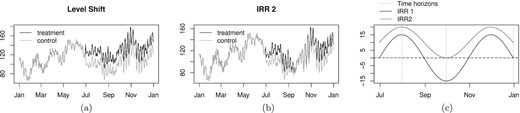
(a) Level shift of +25% for one simulated series; (b) irregular effect (IRR 2); (c) pattern of the irregular effects during all the post-intervention period (those at 1, 3 and 6-month horizons are highlighted in the plot).

In line with the theory presented in Section 4, we tested C-ARIMA and REG-ARIMA in detecting these effects, comparing the performance of both approaches in terms of three indicators: (i) the probability of rejecting the null hypothesis of absence of effect when it is true (type I error probability); (ii) the probability of correctly rejecting the null hypothesis when it is false (power); (iii) computational time. We also tested whether the two approaches would give different results based on the model used in the pre-intervention period (the true model used to generate the data versus the best-fitting model based on the Bayesian Information Criterion) and the time horizon used for valuation (1 month, 3 months and 6 months after the fictional intervention producing the effects).

Table 1 shows the results of simulations in terms of power. Unsurprisingly, REG-ARIMA outperforms C-ARIMA when the effect is a level shift; indeed, the former model is specifically designed for interventions in this form. However, REG-ARIMA fails to detect the negative effect under IRR 1, and incorrectly reject the null of absence of effect at the second time horizon under IRR 2. Conversely, C-ARIMA performs well when the effect is irregular, and does a reasonably good job in case of level shifts compared to benchmark REG-ARIMA, especially when the impact size increases. The simulation results also show that the type I error probability of both approaches is in line with the desired threshold (⁠|$\alpha = 0.05$|⁠) and that C-ARIMA is computationally more efficient than REG-ARIMA. Further comments and additional results are reported in the Online Appendix. Overall, the simulation results indicate that C-ARIMA performs well when the true effect takes the form of a level shift; furthermore, it outperforms the standard REG-ARIMA approach in the estimation of irregular, time-varying effects.

Table 1.

Power of the test based on |$\widehat{\tau }^\dagger _t$| (for C-ARIMA) and |$\widehat{\beta }_D$| (for REG-ARIMA).

	C-ARIMA, |$\tau ^\dagger _t$|							REG-ARIMA, |$\beta _D$|
	TRUE			BIC				TRUE			BIC
	1 m	3 m	6 m	1 m	3 m	6 m		1 m	3 m	6 m	1 m	3 m	6 m
IRR 1	0.480	0.477	0.060	0.482	0.478	0.059		0.052	0.058	0.053	0.054	0.062	0.051
IRR 2	0.724	0.058	0.242	0.726	0.056	0.242		1.000	1.000	1.000	1.000	1.000	1.000
|$+10\%$|	0.243	0.248	0.242	0.243	0.250	0.242		1.000	1.000	1.000	1.000	1.000	1.000
|$+25\%$|	0.895	0.887	0.879	0.895	0.887	0.879		1.000	1.000	1.000	1.000	1.000	1.000
|$+50\%$|	1.000	1.000	1.000	1.000	1.000	1.000		1.000	1.000	1.000	1.000	1.000	1.000

Notes: The numbers in bold highlight when the power function significantly deviates from what is expected (see Figure 1 panel (c)). The results are reported for both the true model (⁠|$TRUE$|⁠) and the best-fitting model (⁠|$BIC$|⁠) at three time horizons: 1 month (1m), 3 months (3m) and 6 months (6m) from the intervention. The different impact sizes ranging from |$+10\%$| to |$+50\%$| in the rows denote estimated effects in the form of level shifts, whereas IRR 1 and IRR 2 indicate the irregular effects.

6. EMPIRICAL APPLICATION

In this section we describe the results of our empirical application; the goal is to estimate the impact of the permanent price reduction performed by an Italian supermarket chain.

6.1. Data and methodology

Data consists of daily sales counts of 11 store brands and their corresponding competitor-brand cookies in the period 1 September 2017–30 April 2019 (Anonymous firm, 2019).¹¹ The permanent price reduction on the store-brand cookies was introduced by the supermarket chain on 4 October 2018. As an example, Figure 2 shows the time series of units sold, the evolution of price per unit and the autocorrelation function of one store brand and its direct competitor. The plots for the remaining store-brand and competitor-brand cookies are provided in the Online Appendix. The occasional price drops before the intervention date indicate temporary promotions run regularly by the supermarket chain. The products exhibit a clear weekly seasonal pattern, evidenced by the spikes in the autocorrelation functions. In the panel referred to the direct competitor brand, we can also observe the evolution of the relative price per unit (the ratio between the prices of the competitor brand and the corresponding store brand). Unsurprisingly, despite the occasional drops due to temporary promotions, the price of the competitor brand relative to the corresponding store brand has increased after the intervention.

Figure 2.

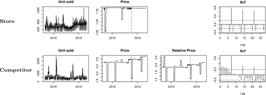
Daily time series of unit sold, price per unit and autocorrelation function for two selected items.

To estimate the causal effect of the permanent price discount on the sales of store-brand cookies, we follow the approach outlined in Section 4. In particular, under the assumptions set out in Section 3, we can analyse each cookie separately, thereby fitting 11 independent models. In order to improve model diagnostics, the dependent variable is the natural log of the daily sales count. This also means that we are postulating the existence of a multiplicative effect of the new price policy on the sales of cookies. Therefore, we focused our attention on estimating the temporal average causal effect, which can still be interpreted as an average multiplicative effect in terms of the original variable. Furthermore, we included covariates to improve prediction of the missing potential outcomes in the absence of intervention. As ruled by Assumption 3.2; all the considered regressors can be safely assumed to be unaffected by the intervention. In particular, to take care of the seasonality we included six dummy variables corresponding to the day of the week and one dummy denoting December Sundays.¹² Indeed, the policy of the supermarket chain implies that all shops are closed on Sunday afternoon, except during Christmas holidays. Thus, we may have two opposite ‘Sunday effects’: a positive effect in December, when the shops are open all day; a negative effect during the rest of the year, since all shops are closed in the afternoon. We also included a holiday dummy taking value 1 before and after a national holiday and 0 otherwise. This is to account for consumers’ tendency to increase purchases before and after a closure day.¹³ Finally, we included a modified version of the unit price, that after the intervention day and during all the post-period is taken equal to the last price before the permanent discount. As explained in the discussion of Assumption 3.2; this is the most likely price that the unit would have had in the absence of intervention. In addition, to estimate the average causal effect of the intervention on store brands, we are also interested in evaluating how this effect evolves with time. Thus, we repeated the analysis by making predictions at three different time horizons: 1 month, 3 months and 6 months after the intervention.

The same methodology is applied to the competitor brands, with a slight modification on the set of covariates. Indeed, this time the unit price is not directly influenced by the intervention, which instead affects the relative price (as shown in Figure 2); so, to forecast competitor sales in the absence of intervention we directly used the actual price.

The results obtained from C-ARIMA are then compared to those of REG-ARIMA. More specifically, we fitted independent linear regressions with ARIMA errors for each of the 11 store brands and their competitors.

6.2. Results and discussion

Table 2 shows the results of the C-ARIMA and the REG-ARIMA approaches applied to the store brands. To provide a more direct comparison with REG-ARIMA, the C-ARIMA results reported here have been derived under the assumption that the error terms are normally distributed. Residuals diagnostics and Normal QQ-plots seem to support this assumption for some of the items (see Figures S5 and S9 in the Online Appendix). In addition, the results based on bootstrapped residuals are in line with those shown in this section for both store and competitor brands (see Tables S6 and S8 in the Online Appendix). Figure 3 illustrates the causal effect, the observed time series and the forecasted series in the absence of intervention for one selected item (additional plots are provided in the Online Appendix). At the 1-month time horizon, the causal effect is significantly positive at the |$5\%$| level for 5 out of 11 items; three months after the intervention, the causal effect is significantly positive at the same level for 8 items; after six months, the effect is significant and positive for 10 items. The analysis performed with REG-ARIMA leads to similar results, except for the effects on items 1 and 2 at the 3-month horizon. This suggests that the intervention might have produced a level shift in the outcome level. To have a summary figure for the impact produced by the permanent price reduction on all store brands, we also estimated the cross-sectional temporal average effect as defined in (3.4). This is positive and significant at all time horizons, indicating that the intervention was, on average, effective in increasing store-brand sales.

Figure 3.

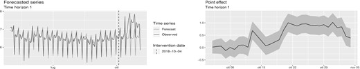
Forecasted sales and pattern of point effect on store brand 4 at 1 month horizon.

Table 2.

Causal effect estimates of the permanent price reduction on store brands.

	Time horizon:
	1 month		3 months		6 months
Item	|$\widehat{\bar{\tau }}^\dagger _t$|	|$\widehat{\beta }_D$|	|$\widehat{\bar{\tau }}^\dagger _t$|	|$\widehat{\beta }_D$|	|$\widehat{\bar{\tau }}^\dagger _t$|	|$\widehat{\beta }_D$|
1	0.14	0.09	0.15.	0.11	0.18**	0.16**
	(0.13)	(0.10)	(0.09)	(0.07)	(0.07)	(0.06)
2	0.14	0.11	0.13	0.13*	0.14*	0.14***
	(0.12)	(0.10)	(0.09)	(0.06)	(0.07)	(0.04)
3	0.19.	0.15.	0.21*	0.18***	0.25***	0.24***
	(0.11)	(0.08)	(0.08)	(0.05)	(0.06)	(0.04)
4	0.49***	0.32***	0.30***	0.22**	0.32***	0.27***
	(0.10)	(0.09)	(0.07)	(0.07)	(0.05)	(0.06)
5	|$-$|0.02	|$-$|0.05	0.07	0.01	0.11	0.07
	(0.13)	(0.09)	(0.10)	(0.07)	(0.07)	(0.05)
6	0.24.	0.25**	0.34***	0.30***	0.37***	0.35***
	(0.12)	(0.09)	(0.09)	(0.07)	(0.07)	(0.05)
7	0.55***	0.57***	0.34***	0.49***	0.30***	0.35***
	(0.11)	(0.04)	(0.08)	(0.09)	(0.06)	(0.04)
8	0.26**	0.33***	0.25***	0.25***	0.14*	0.18**
	(0.08)	(0.07)	(0.07)	(0.07)	(0.06)	(0.06)
9	0.47***	0.56***	0.20***	0.28***	0.21***	0.26***
	(0.07)	(0.07)	(0.05)	(0.08)	(0.04)	(0.06)
10	0.66***	0.82***	0.57***	0.58***	0.33***	0.36***
	(0.12)	(0.12)	(0.10)	(0.05)	(0.08)	(0.06)
11	0.12.	0.11*	0.16*	0.14***	0.14**	0.13***
	(0.06)	(0.05)	(0.06)	(0.03)	(0.05)	(0.03)
|$\widehat{\bar{\tau }}^{(\mathcal {S}) \dagger }_t$|	0.29**		0.25**		0.23***
	(0.11)		(0.08)		(0.06)

Notes:|$^{\boldsymbol{\cdot }}$|p|$\lt $|0.1; |$^{*}$|p|$\lt $|0.05; |$^{**}$|p|$\lt $|0.01; |$^{***}$|p|$\lt $|0.001. The estimates are reported for three different time horizons: 1 month, 3 months and 6 months from the intervention. In this table, |$\widehat{\bar{\tau }}^\dagger _t$| is the estimated temporal average effect (in all models d = D = 0, therefore this is the effect on the original variable and |$\widehat{\bar{\tau }}^\dagger _t = 0$| implies no effect); |$\widehat{\bar{\tau }}^{(\mathcal {S}) \dagger }_t$| is the temporal average effect aggregated across all items; |$\widehat{\beta }_D$| is the coefficient estimate of the intervention dummy according to REG-ARIMA (⁠|$\widehat{\beta }_D = 0$| implies absence of association). Standard errors within parentheses.

Table 3 reports the results for the competitor brands and Figure 4 plots the causal effect, the observed series and the forecasted series for one selected item. Again, the causal effect seems to strengthen as we proceed far away from the intervention.At a 1-month horizon no significant effect is observed; three months after the intervention, on item 10 we find a negative effect and significant at the |$5\%$| level; at a 6-month horizon we find a significant negative effects on item 10 and a significant positive effect on item 5. A negative effect suggests that, following the permanent price discount, consumers have changed their behaviour by privileging the cheaper store brand. Instead, a positive effect might indicate that the price policy has determined an increase in the customer base, i.e., new clients have entered the shop and eventually bought the items at full price. This time, REG-ARIMA leads to different results: at the 6-month horizon, positive effects are found on items 6 and 7, and a negative effect is detected on item 8. This suggests that whatever impact was captured by the intervention dummy of REG-ARIMA, this was not due to the relative price increase experienced by competitor brands. Overall, our analysis on the cross-sectional temporal average effect indicates that competitor brands were mostly unaffected by the intervention applied on store brands.

Figure 4.

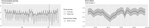
Forecasted sales and pattern of point effect on competitor brand 10 at 1 month horizon.

Table 3.

Causal effect estimates of the permanent price reduction on competitor brands.

	Time horizon:
	1 month		3 months		6 months
Item	|$\widehat{\bar{\tau }}^\dagger _t$|	|$\widehat{\beta }_D$|	|$\widehat{\bar{\tau }}^\dagger _t$|	|$\widehat{\beta }_D$|	|$\widehat{\bar{\tau }}^\dagger _t$|	|$\widehat{\beta }_D$|
1	|$-$|0.04	|$-$|0.03	0.02	|$-$|0.16	0.04	|$-$|0.12
	(0.57)	(0.21)	(0.52)	(0.25)	(0.42)	(0.22)
2	|$-$|0.13	|$-$|0.17	|$-$|0.07	|$-$|0.13	|$-$|0.15	|$-$|0.13
	(0.52)	(0.21)	(0.52)	(0.20)	(0.45)	(0.19)
3	0.04	|$-$|0.06	0.09	|$-$|0.03	0.17	0.01
	(0.42)	(0.22)	(0.32)	(0.20)	(0.21)	(0.17)
4	0.00	0.04	|$-$|0.13	|$-$|0.03	|$-$|0.04	0.01
	(0.31)	(0.19)	(0.23)	(0.16)	(0.18)	(0.13)
5	|$-$|0.03	|$-$|0.02	0.05	0.06	0.12*	0.12**
	(0.11)	(0.06)	(0.07)	(0.06)	(0.05)	(0.05)
6	|$-$|0.05	|$-$|0.01	0.03	0.06	0.09	0.10*
	(0.13)	(0.10)	(0.11)	(0.06)	(0.09)	(0.05)
7	0.04	|$-$|0.11	0.11	|$-$|0.05	0.40	0.39***
	(0.57)	(0.29)	(0.38)	(0.26)	(0.29)	(0.08)
8	|$-$|0.09	|$-$|0.09	|$-$|0.06	−0.07.	|$-$|0.08	−0.10**
	(0.08)	(0.06)	(0.06)	(0.04)	(0.05)	(0.04)
9	|$-$|0.09	|$-$|0.09	|$-$|0.11	|$-$|0.11	|$-$|0.10	|$-$|0.09
	(0.14)	(0.10)	(0.10)	(0.08)	(0.08)	(0.06)
10	|$-$|0.03	|$-$|0.02	−0.12*	−0.09*	−0.11*	−0.08*
	(0.06)	(0.05)	(0.05)	(0.04)	(0.04)	(0.04)
|$\widehat{\bar{\tau }}^{(\mathcal {C}) \dagger }_t$|	|$-$|0.04		|$-$|0.02		0.04
	(0.35)		(0.30)		(0.24)

Notes:|$^{\boldsymbol{\cdot }}$|p|$\lt $|0.1; |$^{*}$|p|$\lt $|0.05; |$^{**}$|p|$\lt $|0.01; |$^{***}$|p|$\lt $|0.001. The estimates are reported for three different time horizons: 1 month, 3 months and 6 months from the intervention. In this table, |$\widehat{\bar{\tau }}^\dagger _t$| is the estimated temporal average effect on the original variable (in all models d = D = 0, therefore this is the effect on the original variable and |$\widehat{\bar{\tau }}^\dagger _t = 0$| implies no effect); |$\widehat{\bar{\tau }}^{(\mathcal {C}) \dagger }_t$| is the temporal average effect aggregated across all items; |$\widehat{\beta }_D$| is the coefficient estimate of the intervention dummy according to REG-ARIMA (⁠|$\widehat{\beta }_D = 0$| implies absence of association). Standard errors within parentheses.

Summarising, the intervention seems to have produced a significant and positive effect on the sales of store-brand cookies. Conversely, we do not find considerable evidence of a detrimental effect on competitor cookies (the only exception being item 10). This indicates that, even though each store-competitor pair is formed by perfect substitutes, price might not be the only factor driving sales. For example, unobserved factors such as individual preferences or brand faithfulness may have a role as well.

7. CONCLUDING REMARKS

We propose a novel approach under the RCM to estimate the effect of interventions in observational time series settings in the absence of untreated units. After a detailed illustration of the assumptions underneath our causal framework, we defined three causal estimands of interest, i.e., the point, cumulative and average causal effects. Then, we introduced a methodology to perform inference. We applied the proposed methodology to estimate the causal effect of the new price policy introduced by a big supermarket chain in Italy, which addressed a selected subset of store-brand products by permanently lowering their price. The empirical analysis was carried out on the goods belonging to the ‘cookies’ category: the results show that the permanent price reduction was effective in increasing store-brand cookies’ sales. Little evidence of a detrimental effect on the corresponding competitor-brand cookies is found.

FUNDING

The authors thank the Department of Excellence 2018-2022 funding provided by the Italian Ministry of University and Research (MUR). The authors also thank the Statistics Department of the University of Florence (DiSIA) and the Florence Center for Data Science.

Footnotes

1

The development version of the CausalArima R package can be accessed from https://github.com/FMenchetti/CausalArima.

2

A notable exception is the method proposed by Chernozhukov et al. (2019), although it requires to observe many control units, and thus it is not applicable in our setting. Related to this, it is worth mentioning that DiD estimators, synthetic control methods and their combinations can be a better choice than C-ARIMA and CausaImpact in case of few pre-treatment periods and multiple treated and control units.

3

This is equivalent to the irreversibility of treatment assumption in Callaway and Sant’Anna (2021). Our persistent treatment is also analogous to the absorbing treatment in Sun and Abraham (2021).

4

This is also known as temporal stable unit treatment value assumption or TSUTVA (Bojinov and Shephard, 2019; Bojinov et al., 2020), which is the time series equivalent of the cross-sectional SUTVA (Rubin, 1974).

5

The supermarket chain sometimes run temporary promotions reducing the price of selected goods for a limited period of time. The time interval after the permanent price discount spans from 4 October 2018 to 30 April 2019, and in the corresponding period before the intervention (4 October 2017 to 30 April 2018) there were no temporary promotions on the store brands that are part of this analysis. Thus, the assumption of a constant price level in the period following the intervention is plausible.

6

Notice that the point effect is analogous to the general causal effect defined in Bojinov and Shephard (2019), with the difference that our estimand is referred to a special setting were the units are subject to a single persistent treatment.

7

Notice that (4.1) can be written in this form because we are assuming absence of within-group interference and absence of additional spillovers, which imply that the potential outcomes of each unit j only depends on its assignment. Conversely, in case these assumptions are not plausible, (4.1) would need to be restated, e.g., by considering a multivariate model. We are also exploiting Assumption 3.1; since we have a single |$\tau _t(1;0)$| in the model equation.

8

The information set at time |$t^{*}$| includes both |$\operatorname{Y}_1(0), \dots , \operatorname{Y}_{t^{*}}(0)$| and |$\operatorname{X}_1, \dots , \operatorname{X}_{t^{*}}$|⁠. Instead, recall that in the post-intervention period we are under Assumption 3.2; meaning that covariates are unaffected by the treatment. Thus, we can consider them as deterministic, which explains why we can take |$\operatorname{X}_{t^{*}+k}^\dagger$| outside the expectation in (4.5).

9

The situation where the ARIMA component of the model is a Random Walk (RW) provides a glaring example of this. In fact,

$$\begin{eqnarray} \widehat{\tau }^\dagger _{t^{*}+1} & =& \Delta \operatorname{Y}_{t^{*}+1} - \widehat{E}[\Delta \operatorname{Y}_{t^{*}+1}(0) | \mathcal {I}_{t^{*}} ] \\ & =& \tau ^\dagger _{t^{*}+1} + \Delta \operatorname{X}_{t^{*}+1}^\prime \left( \beta - \widehat{\beta } \right) + \varepsilon _{t^{*}+1}, \end{eqnarray}$$

but

$$\begin{eqnarray} \operatorname{Y}_{t^{*}+1} - \widehat{E}[\operatorname{Y}_{t^{*}+1}(0) | \mathcal {I}_{t^{*}} ] = \tau _{t^{*}+1} + \operatorname{X}_{t^{*}+1}^\prime \left( \beta - \widehat{\beta } \right) + \varepsilon _{t^{*}+1} \end{eqnarray}$$

so that |$\operatorname{Y}_{t^{*}+1} - \widehat{E}[\operatorname{Y}_{t^{*}+1}(0) | \mathcal {I}_{t^{*}} ] = \widehat{\tau }^\dagger _{t^{*}+1} + \operatorname{X}_{t^{*}}^\prime \left( \beta - \widehat{\beta } \right) \ne \widehat{\tau }^\dagger _{t^{*}+1}$| despite |$\tau _{t^{*}+1} = \tau ^\dagger _{t^{*}+1}$|⁠.

10

Since

$$\begin{eqnarray} (1-L)^d (1-L^s)^D = \sum _{j = 0}^{d+sD} a_j L^j \end{eqnarray}$$

for some |$a_j$| coefficients (⁠|$a_0 = 1$|⁠), then

$$\begin{eqnarray} b_j = -\sum _{i = 0}^{\min \lbrace d+sD;j\rbrace -1} a_i b_{j-i}. \end{eqnarray}$$

For example, if |$d = D = 1$| and |$s = 7$|⁠, then |$\tau _{t^{*}+k} = \tau ^\dagger _{t^{*}+1} + \ldots + \tau ^\dagger _{t^{*}+k}$| for |$k = 1, \ldots , 7$|⁠; |$\tau _{t^{*}+8} = 2\tau ^\dagger _{t^{*}+1} + \tau ^\dagger _{t^{*}+2} + \ldots + \tau ^\dagger _{t^{*}+8}$|⁠, |$\tau _{t^{*}+9} = 2\tau ^\dagger _{t^{*}+1} + 2 \tau ^\dagger _{t^{*}+2} + \tau ^\dagger _{t^{*}+3} + \ldots + \tau ^\dagger _{t^{*}+9}$|⁠, and so on.

11

We excluded the last competitor brand because |$62 \%$| of observations were missing. Thus, we analysed |$J_s = 11$| store and |$J_c = 10$| competitor brands, for a total of |$J = 21$| cookies.

12

We may have a monthly seasonal pattern on top of the weekly cycle, but the reduced length of the pre-intervention series (398 observations) does not allow to assess whether a double seasonality is present.

13

To be precise, on the day of a national holiday we have a missing value (so there is no holiday effect), whereas the dummy variable should capture the effect of additional purchases before and after the closure day(s).

Supporting Information

Additional Supporting Information may be found in the online version of this article at the publisher’s website:

Online Appendix

Replication Package

Notes

Co-editor Dennis Kristensen handled this manuscript.

APPENDIX A: PROOFS OF RESULTS

Proof of Theorem 4.1

Under the assumptions of Theorem 4.1, the maximum likelihood estimator of |$\beta$| can be represented as feasible generalised least squares (FGLS) estimator

$$\begin{eqnarray} \widehat{\beta } = \left( X^{\dagger \prime }_{1} \widehat{R}_{11}^{-1} X^\dagger _{1} \right)^{-1} X^{\dagger \prime }_{1} \widehat{R}_{11}^{-1} y^\dagger _{1}, \end{eqnarray}$$

(A.1)

which can be used to obtain the forecasts on period-2 observations as

$$\begin{eqnarray} \widehat{y}^\dagger _{2} = X^\dagger _{2} \widehat{\beta } + \widehat{z}^\dagger _{2} = X^\dagger _{2} \widehat{\beta } + \widehat{R}_{21} \widehat{R}_{11}^{-1} \widehat{z}^\dagger _{1}, \end{eqnarray}$$

where |$\widehat{z}^\dagger _{1} = y^\dagger _{1} - \widehat{y}^\dagger _{1}$| are the ARMA residuals and the structure of the |$\widehat{z}^\dagger _{2}$| forecasts is implied by the fact that ARMA are linear predictors. Since (A.1) gives

$$\begin{eqnarray} \widehat{\beta } = \beta + \left( X^{\dagger \prime }_{1} \widehat{R}_{11}^{-1} X^\dagger _{1} \right)^{-1} X^{\dagger \prime }_{1} \widehat{R}_{11}^{-1} z^\dagger _{1}, \end{eqnarray}$$

(A.2)

the distribution of the estimator of |$\tau ^\dagger$| is given by

$$\begin{eqnarray} \widehat{\tau }^\dagger & =& y^\dagger _{2} - \widehat{y}^\dagger _{2} \\ & =& \tau ^\dagger + X^\dagger _{2} \beta + z^\dagger _{2} - \left( X^\dagger _{2} \widehat{\beta } + \widehat{R}_{21} \widehat{R}_{11}^{-1} \widehat{z}^\dagger _{1} \right) \\ & =& \tau ^\dagger + z^\dagger _{2} + \left( X^\dagger _{2} - \widehat{R}_{21} \widehat{R}_{11}^{-1} X^\dagger _{1} \right) \left( \beta - \widehat{\beta } \right) - \widehat{R}_{21} \widehat{R}_{11}^{-1} z^\dagger _{1} \\ & =& \tau ^\dagger + z^\dagger _{2} - \underbrace{ \left[ \left( X^\dagger _{2} - \widehat{R}_{21} \widehat{R}_{11}^{-1} X^\dagger _{1} \right) \left(X^{\dagger \prime }_{1} \widehat{R}_{11}^{-1} X^\dagger _{1} \right)^{-1} X^{\dagger \prime }_{1} \widehat{R}_{11}^{-1} + \widehat{R}_{21} \widehat{R}_{11}^{-1} \right] }_{A} z^\dagger _{1}. \end{eqnarray}$$

(A.3)

Equation (A.3) evidences that the dependence of |$\widehat{\tau }^\dagger$| on |$z^\dagger _{1}$| stems partly from the inertia of the ARMA dynamics in the intervention period (the |$-\widehat{R}_{21}\widehat{R}_{11}^{-1} z^\dagger _{1}$| addend) and partly from the dependence of |$\widehat{\beta }$| on the noise |$z^\dagger _{1}$||$\left(\text {the}\, \left( X^\dagger _{2} - \widehat{R}_{21} \widehat{R}_{11}^{-1} X^\dagger _{1} \right) \left( \beta - \widehat{\beta } \right)\, \text {addend}\right)$|⁠. This implies that |$\widehat{\tau }^\dagger$| has mean |$\tau ^\dagger$| and variance

$$\begin{eqnarray} \sigma ^{2}_{z} \left( R_{22} - A R_{12} - R_{21} A^{\prime } + A A^{\prime } \right). \end{eqnarray}$$

Finally, (A.3) allows us to interpret the contribution of the different addends in determining the behaviour of |$\widehat{\tau }^\dagger$|⁠. In case |$\widehat{R}_{21}$| and |$\widehat{R}_{11}$| are substituted with their true counterparts (we recall that we are assuming that model parameters are consistently estimated), nothing changes substantially. Differently, replacing |$\widehat{\beta }$| by |$\beta$| suppresses the dependence on |$z^\dagger _1$| that is instead apparent from (A.3). It is true that, differently from the other addends, the role of |$\left( X^\dagger _{2} - \widehat{R}_{21} \widehat{R}_{11}^{-1} X^\dagger _{1} \right) \left( \beta - \widehat{\beta } \right)$| vanishes with the sample size, but is also true that its weight can be important in relatively small samples. |$\square$|

Identification proof We prove that under Assumption 3.3; the point causal effect is identifiable from available data. To simplify the notation while deriving of the proof, we drop the j subscript from the outcome and the effect. By Definition 3.1,

$$\begin{eqnarray} \tau _{t^{*}+k} & = \operatorname{Y}_{t^{*}+k}(1) - \operatorname{Y}_{t^{*}+k}(0) \end{eqnarray}$$

(A.4)

$$\begin{eqnarray} = \operatorname{Y}_{t^{*}+k}(1) - E[\operatorname{Y}_{t^{*}+k}(0) | \mathcal {I}_{t^{*}}] \end{eqnarray}$$

(A.5)

is the point causal effect at time |$t^{*}+k$|⁠. The quantity |$\operatorname{Y}_{t^{*}+k}(1)$| is immediately identified from the available data, since it is the observed outcome. We now show that, under Assumption 3.3 the second quantity is identifiable from the data as well.

Let |$\mathcal {I}_{0}$| denotes the information set up to time |$t = 0$| and define |$\mathcal {I}_{t^{*}} = \lbrace \mathcal {I}_{0}, \operatorname{X}_{1}, \dots , \operatorname{X}_{t^{*}}, \operatorname{Y}_{1}(0), \dots , \operatorname{Y}_{t^{*}}(0) \rbrace$|⁠. At time |$t^{*}+1$| this relation follows directly from Assumption 3.3:

$$\begin{eqnarray} f_{\operatorname{Y}_{t^{*}+1}|\mathcal {I}_{t^{*}}} (y_{t^{*}+1}|\mathcal {I}_{t^{*}}) = f_{\operatorname{Y}_{1} | \mathcal {I}_{0}} (y_{t^{*}+1}|\mathcal {I}_{t^{*}}). \end{eqnarray}$$

(A.6)

Therefore, assume we know the density at time |$t=1$| (conditioning on the information up to |$t=0$|⁠) by learning from observed data. Then, under conditional stationarity we would also know the density at time |$t^{*}+1$| (conditioning on the information up to |$t = t^{*}$|⁠). Similarly, at time |$t^{*}+2$| we have,

$$\begin{eqnarray} f_{\operatorname{Y}_{t^{*}+2}|\mathcal {I}_{t^{*}}} (y_{t^{*}+2}|\mathcal {I}_{t^{*}}) & =& \int f_{\operatorname{Y}_{t^{*}+2}|\operatorname{Y}_{t^{*}+1}, \mathcal {I}_{t^{*}}} (y_{t^{*}+2}|y_{t^{*}+1}, \mathcal {I}_{t^{*}}) f_{\operatorname{Y}_{t^{*}+1}|\mathcal {I}_{t^{*}}} (y_{t^{*}+1}|\mathcal {I}_{t^{*}}) d y_{t^{*}+1} \\ & =& \int f_{\operatorname{Y}_{t^{*}+1}|\mathcal {I}_{t^{*}}} (y_{t^{*}+2}|y_{t^{*}+1}, \mathcal {I}_{t^{*}}) f_{\operatorname{Y}_{t^{*}+1}|\mathcal {I}_{t^{*}}} (y_{t^{*}+1}|\mathcal {I}_{t^{*}}) d y_{t^{*}+1}, \end{eqnarray}$$

(A.7)

where, again, the last equality follows from Assumption 3.3. Therefore, the density at time |$t^{*}+2$| is identifiable from observed data. The proof for a generic time |$t^{*}+k$| follows analogously by induction. Notice, however, that the assumption of absence of anticipatory effects is implicit in the conditional stationarity assumption. Indeed, if |$\operatorname{Y}_{t}(0)$| is influenced by the intervention for some |$t \le t^{*}$|⁠, this would result in a change in the density function and the conditional stationary assumption would no longer be valid. |$\square$|