Towards assessment of cork production through National Forest Inventories

Abstract

The economic importance of cork in the Mediterranean region demands an accurate assessment of its production. Cork production is currently estimated by aggregating information provided by Regional Forest Services, but this approach results in a lack of robustness at the national level. The objective of the present study is to analyse the role of the Spanish National Forest Inventory (SNFI) as a potential source of data for quantifying cork weight at national level and the scope of National Forest Inventory data to define national trends in cork yield as well as to characterize the main types of cork producing forest stands in Spain. Data from the Second and Third SNFI are used together with the Spanish Forest Map. The results point to the suitability of SNFI to quantify cork production as long as the two main variables defining cork weight, namely cork thickness and debarking height, were correctly recorded in inventories. Although the Second SNFI complied with these requirements, from the Third SNFI the methodology changed, preventing the accurate estimation of cork weight. Based on this study recommendations are made to improve the estimation of cork weight at national level, e.g. to measure cork thickness in all the cork oaks in the plot and to take a sample of cork from the inventoried trees. This information would also make it possible to assess the cork quality in terms of cork thickness growth and to classify cork production in terms of suitability for producing high quality cork products.

Introduction

Today, the importance of non-wood forest products (NWFPs) is beyond any doubt (Wolfslehner et al., 2013). These goods are not only important from a recreational point of view, in close association with the traditional use of forests as a source of livelihood, but are also highly profitable from a commercial perspective (Masiero et al., 2016). NWFP occupy an important place in the livelihood of rural communities through the sale of products as well as auto-consumption (Nasi et al., 2002), the economic revenue created often being greater than that generated by timber production (Palahí et al., 2009; Miina et al., 2010; Pasalodos-Tato et al., 2016). Additionally, some authors highlight the large unused potential of NWFP to support rural development and increase the income of land owners and rural enterprises (Ludvig et al., 2016). In Europe, Christmas trees, fruits, berries and cork are the most important NWFPs from an economic standpoint (Forest Europe, UNECE and FAO, 2011). The EU accounts for 80 per cent of the worldwide production of cork (Pelli et al., 2009; Sierra-Pérez et al., 2015), with an area of ~1.7 million ha of cork oak forests, mainly in Portugal and Spain, generating revenues of 325 million euros at the European level (Pereira, 2011). In addition, cork oak stands play a key role in the economies of the regions in which they are found, not only due to the direct economic benefits from cork production, but also because of indirect benefits derived from activities associated with this type of forests such as hunting, cattle grazing or other products such as firewood and acorns. In this context, it is important to have accurate estimates of cork production, not only for the industrial sector to establish business strategies but also to comply with international reporting requirements for Forest Europe and FAO (Forest Resource Assessment – FRA). Similarly, it is important to keep a continuous record of cork production at regional and national level so that the production trends shown by this commodity can be monitored. One possible approach to quantifying cork production would be to use National Forest Inventories (NFI), especially bearing in mind the multipurpose character they have acquired in recent years (Corona et al., 2011; Alberdi et al., 2017) as a tool to address the challenges posed by new environmental policies and the needs of society. Moreover, given the current effort being channelled towards harmonizing different indicators at European level (Winter et al., 2008; Ståhl et al., 2012; Tomppo and Schadauer, 2012) it would seem sensible to use this NFI data to estimate cork production and develop appropriate sustainability indicators for these forests at national level.

In Spain, national cork production is estimated by aggregating the information provided by Regional Forest Services. Therefore, greater robustness of the data at national level is needed. The Spanish National Forest Inventory (SNFI) provides consistent forest information, although it has never been used to estimate cork production. Within this framework, the first step towards quantifying cork production at national level is to analyse the information provided by the SNFI to test whether this type of data are suitable or at least to identify the limitations of SNFI data for this purpose. Additionally, it would be of interest to characterize the forest stands devoted to cork production. In Spain there are two main types of stands producing cork, namely ‘cork oak stands' and dehesas (agro-silvopastoral systems). Cork oak stands are denser and the trees tend to be thinner than those in dehesas, which are open woodlands, but to date no definitive reference values based on quantitative analyses have been provided to characterize these stands properly. It is worth noting than the term 'cork production' refers to the cork that has been harvested. In this study, the focus is on the standing cork, which could be estimated using SNFI. Thus the term 'cork weight' is used to quantify the amount of cork under debarking height growing in the forests (i.e. able to be harvested) when the SNFI was performed.

The objectives of the present study are to: (i) analyse the suitability of SNFI for estimating cork weight at national level; (ii) test the role of SNFI in depicting trends in cork weight at national level and (iii) characterize the main types of forest stands that produce cork in Spain using SNFI and the Spanish Forest Map (SFM, MAAMA, 1997–2006) as information sources.

Material and methods

Dataset

Data from the Second (2SNFI, 1986–1996) and Third (3SNFI, 1997–2007) National Forest Inventories were used to conduct the present study. The SNFI consists of a systematic network of permanent plots distributed on a grid of 1 km square cells and with a planned remeasurement interval of 10 years. Each permanent plot comprises four concentric sub-plots with radii of 5, 10, 15 and 25 m in which the minimum dbh (diameter at breast height) recorded are 75, 125, 225 and 425 mm, respectively. More information regarding technical aspects of Spanish NFI can be accessed in Alberdi Asensio et al. (2010), MMA (1990) and Villanueva (2004).

In these SNFI plots, in addition to tree variables (namely diameter at breast height (dbh) and tree height (H)), when the tree species inventoried was cork oak, a so-called ‘special parameter’ was recorded indicating whether the tree had been debarked. If it had, then a record was taken of whether the stem and branches had been debarked or not as well as the debarking height (DH). In the plots from the 2SNFI, the cork thickness was measured in 1–6 trees per plot, thus allowing the volume of cork on those trees to be calculated (see equation (1) for further details). It was assumed that the rest of the cork oaks in the same plot had the same cork thickness, which was the arithmetic mean of the cork thickness of the inventoried trees. However, in the 3SNFI, unlike the 2SNFI, cork thickness was not measured and therefore it is not possible to directly estimate the volume of cork on those trees. In order to fulfil the objectives of the study, the dataset employed was composed of SNFI monitored plots that included at least one cork oak with diameter higher than 20 cm in the production phase (i.e. that had been debarked at least once in 2SNFI). In order to allow comparisons to be drawn between both SNFI, the same trees were analysed in the 2SNFI and 3SFNI, thus those trees that died between 2SNFI and 3SNFI were not considered in the study. In accordance with this criterion, the number of plots considered was 2109 with a total of 10 543 cork oaks. The dataset included plots with both pure and mixed cork oak stands. Finally, the complete dataset used in the present study (Table 1) comprises the main stand variables, namely stand basal area (G, m² ha⁻¹), mean quadratic diameter (dg, cm) and number of trees per hectare (N, stems ha⁻¹), as well as the tree variables recorded: diameter at breast height (dbh, cm), tree height (H, m), debarking height (DH, m) and, in the case of trees from the 2SNFI, cork thickness (ct, mm).

Table 1

Characterization of the main stand and tree-level variables of plots in the 2SNFI and 3SNFI according to their mean (Mean), minimum (Min), maximum (Maxi) values and standard deviation (Std. dev.)

Variable	2SNFI					3SNFI
	#	Min	Maxi	Mean	Std. dev.	#	Min	Maxi	Mean	Std. dev.
G (m2 ha−1)	2109	0.42	53.12	11.17	8.01	2109	0.51	62.07	13.73	9.25
dg (cm)	2109	7.95	146.50	32.66	17.09	2109	8.87	147.40	34.11	17.14
N (stems ha−1)	2109	5.09	2974.43	342.57	418.87	2109	5.09	3263	405.35	474.37
Grel (%)	2109	0.37	100	61.40	37.12	2109	1.38	100	65.45	32.62
Nrel (%)	2109	1.36	100	67.31	33.17	2109	0.33	100	58.06	37.05
dbh (cm)	2109	13.00	127.30	37.96	14.67	2109	9.10	135.6	41.38	16.12
H (m)	2109	4.00	25.00	8.46	2.34	2109	0	25.00	8.78	2.65
DH (m)	2109	0	10.00	2.35	1.70	2109	0	10.00	2.34	1.68
ct (mm)	2109	11.00	70.00	24.92	11.49	–	–	–	–	–

Here # is the number of plots, G is the basal area of the plot, dg is the quadratic mean diameter, N is the stand density, G_rel is the relative basal area of the cork oaks in the plot (%), N_rel is the relative stand density of the cork oaks in the plot (%), dbh is the diameter at breast height, H is the height of the tree, DH is the debarking height and ct is the cork thickness.

Cork weight estimation and trend followed

SNFI plot level

To estimate cork weight in the plots belonging to the 2SNFI or the 3SNFI, two different approaches were applied depending on the data available. Although there is an extensive work on individual cork production models (see Vázquez-Piqué and Pereira, 2008 for references), the variables recorded in the 2SNFI in relation to cork production (debarking height (DH) and cork thickness (ct)) were not compatible with any of these models. It was assumed that the shape of the trunk was cylindrical based on the work of Montero (1987) that introduced the concept of shape coefficient. The shape coefficient (Montero, 1987) is the relationship between the real debarking surface and the debarking surface if the stem was cylindrical, this coefficient being equal to 1 when debarking height is equal to 2.6 m and branches were not debarked. In our case the average debarking height in the trees considered were 2.39 and 2.41, for 2SNFI and 3SNFI respectively (Table 1). Based on this it was considered that the assumption of equalling the stem to a cylinder was justified. Therefore, the volume of cork of an individual tree was estimated using the following equation:

$$V_{\mathrm{c}\mathrm{o}\mathrm{r}\mathrm{k}}=\mathrm{D}\mathrm{H}\cdot \mathrm{c}\mathrm{t}\cdot \mathrm{p}\mathrm{b}\mathrm{h}$$

(1)

where DH is the debarking height (m), ct is the cork thickness (m) and pbh is the stem circumference at breast height under bark (m). By multiplying the volume of cork (V_cork (m³)) by the cork density (kg m⁻³), the cork weight for every tree is obtained. Cork density present a high variability not only among trees but also within the same tree because it depends on cork cell features as cell size and cell wall corrugation, the proportion of early-cork and late-cork in the annual ring, the extent of porosity and inclusions and discontinuities (Pereira, 2011). In the study a mean value of cork density accepted in the literature of 251 kg m⁻³ was used to calculate cork weight (Pereira, 2011). The sum of the cork weight of all the trees in the plot gives the cork weight per plot.

In the case of the 3SNFI, the cork thickness was not recorded and only the debarking height was available. To estimate the cork thickness in the trees from the 3SNFI, data from the 2SNFI were used as the starting point for the calculations: diameter under cork and the cork thickness of all the cork trees. With this information, the annual diameter increment of these trees was estimated by means of the model developed by Sánchez-González et al. (2006):

$$\widehat{i{\mathit{d}}_{\mathit{u}}}=0.18+7.89\frac{1}{N}-1.02\frac{1}{\mathrm{SI}}+2.45\frac{1}{\mathrm{du}}$$

(2)

where $\widehat{i{d}_u}$ is the estimated annual diameter increment under cork (cm), N is the number of trees per hectare (trees ha⁻¹), SI is the site index (m) and du is the diameter at breast height under cork at the 2SNFI, which is obtained by subtracting twice the arithmetic mean of the cork thickness of the inventoried trees from the measured diameter over cork of each tree. Since this model is recommended for use in cork stands that have a du higher than 20 cm, it was only used on trees of that size. All the variables included in the model are directly provided by the plots of the SNFI except the SI, which must be computed for each plot using the model for height growth of the dominant trees (Sánchez-González et al., 2005):

$$H=\frac{20.7216}{1-\left(1-\frac{20.7216}{\mathrm{S}\mathrm{I}}\right)\cdot {\left(\frac{80}{T}\right)}^{1.4486}}$$

(3)

where H is dominant height (m) and T is stand age (years) and SI is the site index (m).

Once the SI has been estimated for each plot, the annual diameter increment under cork of each cork oak tree from the plots of the 2SNFI is calculated. From this increment, the theoretical diameter under cork at the 3SNFI is estimated according to the following expression:

$$\widehat{\mathit{d}{\mathit{u}}_{3\mathrm{SNFI}}}=\mathit{d}{\mathit{u}}_{2\mathrm{SNFI}}+n\cdot i{\mathit{d}}_{\mathit{u}}$$

(4)

where $\widehat{d{u}_{3\mathrm{S}\mathrm{N}\mathrm{F}\mathrm{I}}}$$$is the estimated diameter at breast height under cork in the 3SNFI, du_2SNFI is the real diameter at breast height under cork in the 2SNFI, n is the number of years between the 2SNFI and the 3SNFI and id_u is the annual diameter increment under cork (cm) of the 2SNFI.

The difference between the estimated du_3SNFI and the diameter over cork provided by the plots of the 3SNFI is the cork thickness (ct) for the trees in the 3SNFI plots. Figure 1 shows an explanatory diagram to clarify the estimation of the diameter under cork in each SNFI. From the estimated cork thickness and the DH reported in the 3SNFI plots, the cork weight per plot can be estimated according to equation (1).

Figure 1

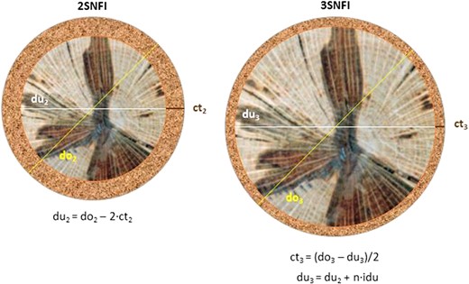
Explanatory diagram to clarify the estimation of the diameter under cork dui in each SNFI. ct2 is the measured cork thickness for trees on which this measurement was taken in the 2SNFI, while for the rest of the trees in the same plot this figure is taken as the arithmetic mean of the cork thickness of the inventoried trees. doi is the diameter over cork, which is the only variable that was measured on all trees at both SNFI. N is the number of years between the 2SNFI and the 3SNFI. idu is the annual diameter increment which is estimated using the model developed by Sánchez-González et al. (2006).

National level

Based on the calculations described above, cork weight was estimated for all productive cork oaks in both the 2SNFI and the 3SNFI. In order to estimate what these values represent at national level, the plot-level estimates of cork weight must be scaled up to landscape level. The categorical units chosen for this purpose were the forest types (FT), taken from the Spanish Forest Map (SFM, scale 1:50.000) (MAAMA, 1997–2006; Vallejo, 2005). The SFM is the cartographic ‘pillar’ of the SNFI (in this case from the 3SNFI) and is produced through the photointerpretation of orthophotos together with fieldwork (at least 10 per cent of the polygons are visited) so that a classification of the territory into homogenous polygons is obtained. In the SFM, 73 FT are categorized according to the dominant species, canopy cover, management and development stage (IEPNB, 2011). The selected dataset plots from the 3SNFI were classified according to the SFM FTs. Taking into account the sampling design of the 3SNFI and the relative number of plots of each FT in the dataset, the forest area containing cork oaks in the production phase was estimated. As regards the 2SNFI2, the same study area was considered as ‘forest land remaining forest land’ (Penman et al., 2003) in the 3SNFI to avoid errors caused by methodological differences in the accuracy of the cartography used in each NFI cycle. Additionally, it was assumed that each plot maintained the same FT in both inventories.

Characterization of the productive cork stands according to different FT

In addition to estimating the cork weight per FT at national level and identifying the trend between the 2SNFI and the 3SNFI, it is also important to define the main characteristics of the cork producing stands in Spain. This objective is assessed by using the FTs from the SFM. Among the variables that serve to characterize these FT are all the variables related to the production of cork (ct, DH), relevant tree level variables (dbh, H) and stand level variables that describe the stand structure and its specific composition, for instance stand density (N), basal area (G) as well as their relative values expressed as a percentage of the total N (N_rel) and G (G_rel), respectively. The values adopted by these variables serve as reference values to characterize those stands capable of producing cork. The FT where cork oaks were found, together with the area occupied by each, is presented in Figure 2 and Table 2, respectively. González-Adrados (2015) found values of 689 000 has for pure Quercus suber stands and mixed stands of Q. suber and Quercus ilex. This result is in line with our estimation based on the SFM that only considered areas with cork oaks in the production phase instead of any cork oak.

Table 2

Description of the main forest types (FT) producing cork and the area covered by each type according 3SNFI

Forest types	Description	Area (ha)
Q. suber stands	Forests dominated by Q. suber (representing at least 70% of the canopy cover)	208 741.34
Dehesas	Forest with generally incomplete fraction of canopy cover and well-developed herbaceous layer, whose main product is the extensive use not only livestock with arable pasture, but also the woody plant fruits. Agro-forestry-pastoral system in which the management of extensive livestock is used as a conservation and improvement tool	239 732.00
Broadleaves mixed forests in the Mediterranean biogeographic region	Mixed forests composed by broadleaves located in the Mediterranean biogeographical region	114 300.11
Autochthonous broadleaves and conifer mixed forests in the Mediterranean biogeographic region	Mixed forests composed by autochthonous broadleaves and conifers located in the Mediterranean biogeographical region	40 181.32
Q. ilex stands	Forests dominated by Q. ilex (representing at least 70% of the canopy cover)	50 936.39
Other FT		59 373.99
Total		713 265.15

Figure 2

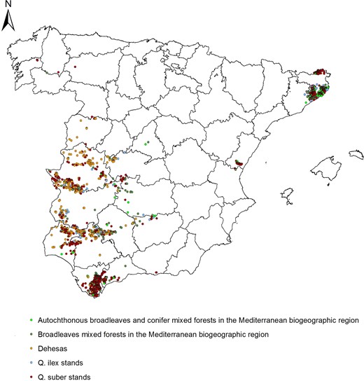
Distribution of the SNFI plots characterized by the FT they belong to.

Results and discussion

Cork weight estimation and trends

SNFI plot level

The results (Table 3) show that ct is significantly smaller in the 3SNFI, meaning that the cork weight is much lower in the 3SNFI than in the 2SNFI (Table 3). When the variables related to cork thickness estimation at plot level are disaggregated into diameter classes, it can be seen that cork thickness in the 3SNFI is greater for diameter classes above 120 (Figure 3). Negative values of cork thickness were found in the smaller diameter classes, mainly due to different sources of error that affect the estimation of diameter under cork (du_3SNFI). Firstly, measurement errors derived from the uneven morphology of the cork. Secondly, errors derived from the assumption that the rest of the cork oaks in the same plot at the 2SNFI had the same cork thickness, which was the arithmetic mean of the cork thickness of the inventoried trees. This assumption led to incorrect estimation of the initial diameter under cork used to estimate the annual diameter increment. This source of error is especially relevant: (i) in those plots with cork oaks belonging to different diameter classes; (ii) in those plots that include both cork oaks that have never been debarked and cork oaks that have already been debarked, and (iii) in those trees of which cork age is very different in both inventories; for example, those trees that were about to be debarked in the 2SNFI but were already debarked in the 3SFNI. Thirdly, the error associated with applying the diameter increment model equation (2) to estimate the du in the 3SNFI. This model is recommended for use in cork stands with trees that have a du between 20 and 80 cm and have been debarked at least three times, in other words, in stands that only produce mature cork (also termed ‘reproduction cork’), which is that obtained from the third debarking onwards. That is the reason why it was decided to remove cork oak trees smaller than 20 cm of du from the analysis. However, it was also decided not to remove trees bigger than 80 cm because the error committed in those trees when estimating the annual diameter increment is negligible due to the low growth rate in older trees. In addition, those models were developed using data from the two main areas in Spain with dense cork oak forests, Catalonia and Los Alcornocales Natural Park. The suitability of this model to dehesas has not been tested and it is possible that in those stands the performance would be inferior (Sánchez-González et al., 2006). Although negative values of cork thickness are meaningless as far as cork estimation purpose is concerned, it was decided to show these results to illustrate that cork weight cannot be estimated without an accurate measurement of cork thickness.

Table 3

Characterization of the main variables related to cork production in the 2SNFI and 3SNFI according to their mean (Mean), minimum (Min), maximum (Maxi) values and standard deviation (Std. dev.)

Variables	2SNFI					3SNFI
	#	Min	Max	Mean	Std. dev.	#	Min	Max	Mean	Std. dev.
dbh (cm)	1728	20.00	127.30	39.36	13.71	1728	20.65	135.60	43.54	15.11
H (m)	1728	3.50	17.30	8.70	2.19	1728	4.00	17.00	9.26	2.15
DH (m)	1728	0.10	9.90	2.54	1.69	1728	0.50	9.90	2.50	1.68
ct (mm)	1728	1.00	67.50	24.63	11.82	1728	−90.20	87.17	9.14	11.66
wcork (kg ha–1)	1728	4.00	8790.61	807.80	892.11	1728	−695.63	7630.49	349.52	586.23

Here # is the number of plots, dbh is the diameter at breast height, H is the height of the tree, DH is the debarking height, ct is the cork thickness and w_cork is the cork weight. All the variables have been measured except ct in 3SNFI plots and w_cork in 2SNFI and 3SNFI which have been estimated based on the measured variables.

Figure 3

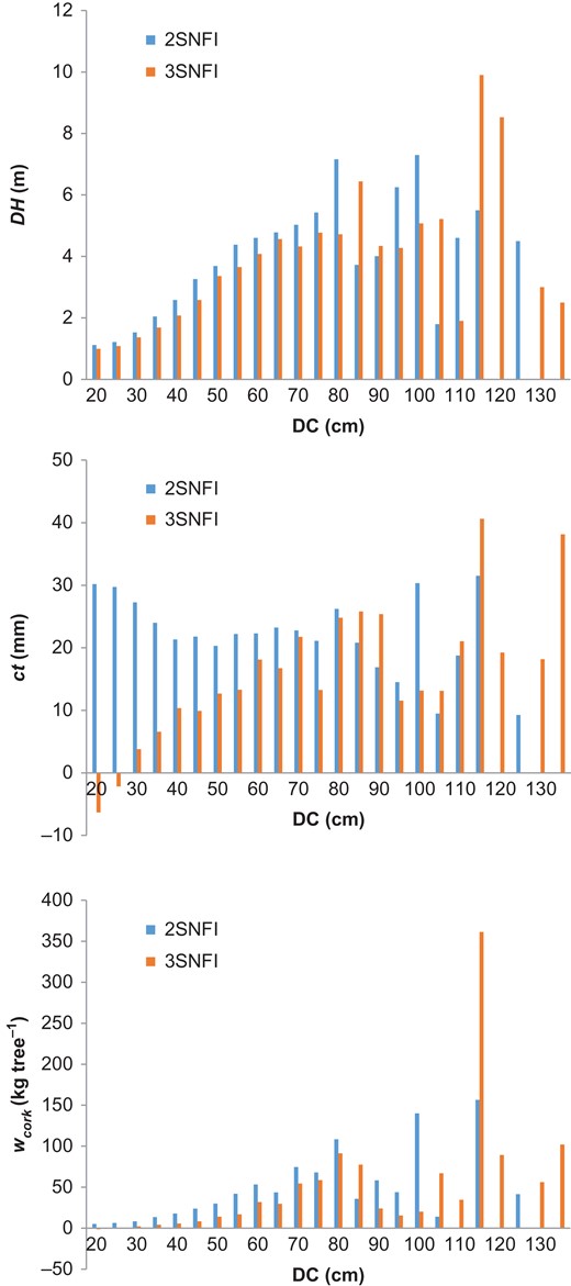
Mean values per diameter class over cork (DC) of the main cork-production related variables: debarking height (DH), cork thickness (ct) and the cork weight (w_cork).

Notable differences between the 2SNFI and the 3SNFI are still evident even where the variables are classified according to different site indices (SI) (Table 4). In this regard, the results indicate that there is no direct relationship between site index (SI) and cork-production related variables, confirming the results found in the literature (Almeida et al., 2010). Although the plots with the highest mean cork weight values are those belonging to SI 14 m, the amount of cork produced by stands with SI 6 m is almost the same, closely followed by stands with SI 12 m, 10 m and 8 m, respectively. The same pattern is found in the case of ct, with all the SI presenting very similar values of mean ct, which indicates that SI and ct are not directly related either. Furthermore, ct is a good indicator of the cork production quality of a stand (Paulo et al., 2017), hence, a national level cork quality map could be produced if the age of the cork were recorded when performing the stand inventory. This type of characterization is not currently possible with the available data.

Table 4

Characterization of the main variables related to cork production in the 2SNFI and 3SNFI according to their mean (Mean), minimum (Min), maximum (Maxi) values and standard deviation (Std. dev.) according to different site indices (SI)

SI	Variable	2SNFI					3SNFI
		#	Minimum	Maximum	Mean	Std. deviation	#	Minimum	Maximum	Mean	Std. deviation
6	dbh (mm)	787	200.00	1273.00	378.22	136.38	780	206.50	1356.00	415.62	148.66
	H (m)	787	3.50	17.30	8.53	2.16	773	4.00	16.20	8.45	1.90
	DH (m)	778	0.10	9.90	2.39	1.58	762	0.50	9.90	2.35	1.58
	ct (mm)	756	1.00	67.50	24.73	12.07	749	−90.20	80.25	9.52	11.04
	wcork (kg ha−1)	787	11.78	5701.77	795.84	893.86	787	−244.84	7630.49	362.71	637.21
8	dbh (mm)	331	209.50	987.00	371.89	117.54	330	224.00	1066.00	413.86	129.75
	H (m)	331	4.50	14.00	8.18	1.89	328	5.30	13.64	8.62	1.68
	DH (m)	330	0.60	9.90	2.33	1.51	316	0.60	9.90	2.37	1.49
	ct (mm)	331	2.50	57.00	24.44	11.45	331	−22.79	44.39	9.50	10.97
	wcork (kg ha−1)	331	17.57	5214.10	703.68	773.87	331	−365.79	4067.20	309.47	480.96
10	dbh (mm)	295	202.50	1241.00	387.60	134.18	292	207.50	1305.00	427.33	145.10
	H (m)	295	4.00	16.33	8.49	2.07	292	5.40	15.57	9.17	1.79
	DH (m)	290	0.70	9.90	2.48	1.65	286	0.70	9.90	2.42	1.56
	ct (mm)	287	1.00	54.13	25.00	11.49	284	−65.54	43.50	6.92	11.03
	wcork (kg ha−1)	295	27.40	5136.55	825.36	841.20	295	−430.58	2735.60	282.96	452.25
12	dbh (mm)	273	224.50	1028.00	402.00	137.98	272	239.00	1098.00	448.72	153.17
	H (m)	273	4.42	15.00	8.77	2.10	270	5.88	15.50	9.79	1.86
	DH (m)	271	0.70	9.20	2.64	1.80	263	0.70	9.50	8.92	1.76
	ct (mm)	260	1.00	62.50	24.77	12.56	259	−40.49	87.17	2.62	13.01
	wcork (kg ha−1)	273	4.00	8790.61	837.70	1015.66	273	−461.01	3041.66	331.80	531.24
14	dbh (mm)	380	216.00	987.00	446.16	144.14	376	236.00	1139.00	495.82	161.94
	H (m)	380	4.75	16.25	9.69	2.39	372	7.00	17.00	11.31	2.11
	DH (m)	374	0.50	9.90	3.01	1.94	360	0.50	9.90	2.94	1.98
	ct (mm)	370	1.00	57.50	24.15	11.36	366	−29.20	60.36	9.98	12.84
	wcork (kg ha−1)	380	6.54	5891.80	895.38	929.34	380	−695.63	6300.78	425.96	681.84

Here # is number of plots, dbh is the diameter at breast height, H is the height of the tree, DH is the debarking height, ct is the cork thickness and w_cork is the cork weight. All the variables have been measured except ct in 3SNFI plots and w_cork in 2SNFI and 3SNFI which have been estimated based on the measured variables.

National level

Apart from the mean values presented in the previous sections, it is highly important to have accurate estimations of the cork weight produced at national level in Spain. Cork oaks in the production phase belong to different FTs, in which cork production may or may not be the main management objective. In the case of cork oak stands and dehesas (agro-silvopastoral systems), cork oak is the dominant species, as can be observed from the Grel and Nrel values presented by these stands (Table 5), hence their management is oriented towards cork production. However, there are other FTs in which cork oak is not the main species, such as ‘Broadleaf mixed forests in the Mediterranean biogeographic region', ‘Autochthonous broadleaf and conifer mixed forests in the Mediterranean biogeographic region' and ‘Quercus ilex stands'. The mean cork weight estimations at FT level are presented in Table 5. According to these results, a clear pattern can be identified; all the FT present higher values for cork weight in the 2SNFI than in the 3SNFI. For instance, in Quercus suber stands (the main cork producing FT), cork weight in the 3SNFI drops to 55 per cent of that obtained in the 2SNFI. A similar decline (62 per cent) is found for the Broadleaf mixed forests in the Mediterranean biogeographic region FT. Still more notable are the cases Autochthonous broadleaf and conifer mixed forests in the Mediterranean biogeographic region FT in which the reduction is 72 per cent while in dehesas and Quercus ilex stands cork weight only falls by 38 and 46 per cent, respectively, between the 2SNFI and the 3SNFI.

Table 5

Statistics relating to cork weight production and the main stand variables selected for the Forest type (FT) analysed according to their mean (Mean), minimum (Min), maximum (Maxi) values and standard deviation (Std. dev.)

FT	Variable	2SNFI					3SNFI
		#	Min	Max	Mean	Std. dev.	Min	Max	Mean	Std. dev.
Q. suber stands	dbh (mm)	880	211.00	1146.00	378.14	112.14	210.50	1187.00	418.40	122.99
	H (m)	880	3.50	16.00	8.74	2.26	4.00	16.20	9.29	2.14
	DH (m)	880	0.50	9.90	2.45	1.55	0.50	9.90	2.42	1.52
	ct (mm)	880	1.00	54.13	23.40	10.55	−65.54	50.12	8.79	10.55
	wcork (kg ha−1)	880	4.00	8790.61	1056.99	1063.79	−430.58	7630.49	480.25	745.35
	N (trees ha−1)	880	5	2189	216	238	5	2310	224	244
	G (m2 ha−1)	880	0.85	40.83	12.45	6.88	1.06	51.24	14.42	7.90
	Nrel (%)	880	1.13	100.00	87.04	22.80	1.96	100.00	83.34	25.46
	Grel (%)	880	14.25	100.00	91.71	14.53	6.79	100.00	90.21	14.87
Dehesas	dbh (mm)	340	209.50	1106.50	485.06	143.39	255.00	1201.50	540.50	154.89
	H (m)	340	5.00	14.79	8.50	1.77	4.50	14.65	9.07	1.77
	DH (m)	338	0.60	9.90	3.67	1.84	0.90	9.90	3.69	1.89
	ct (mm)	340	1.00	51.50	18.45	9.17	−34.93	87.17	13.00	10.94
	wcork (kg ha−1)	340	10.39	4388.34	733.76	783.70	−111.25	4185.97	455.42	607.76
	N (trees ha−1)	340	5	343	47	47	5	302	46	45
	G (m2 ha−1)	340	0.67	21.29	6.19	4.16	0.74	22.46	6.94	4.53
	Nrel (%)	340	1.83	100.00	64.25	35.38	1.17	100.00	63.71	35.70
	Grel (%)	340	5.87	100.00	72.47	29.08	6.50	100.00	72.46	28.98
Broadleaves mixed forests in the Mediterranean biogeographic region	dbh (mm)	261	201.00	779.33	397.20	128.39	207.00	825.00	437.49	141.18
	H (m)	261	4.00	16.00	8.95	2.27	4.50	17.00	9.59	2.33
	DH (m)	259	0.80	8.84	2.42	1.56	0.80	8.40	2.32	1.39
	ct (mm)	261	1.00	54.50	24.72	11.64	−24.66	80.25	9.68	12.70
	wcork (kg ha−1)	261	6.54	4947.89	607.81	711.77	−144.81	1595.02	229.29	323.00
	N (trees ha−1)	261	5	787	113	139	5	774	122	152
	G (m2 ha−1)	261	0.63	28.50	6.44	4.43	0.67	21.85	7.26	4.55
	Nrel (%)	261	1.47	100.00	40.14	29.56	1.37	100.00	35.62	26.92
	Grel (%)	261	11.52	100.00	58.47	23.66	10.07	100.00	54.73	21.54
Autochthonous broadleaves and conifer mixed forests in the Mediterranean biogeographic region	dbh (mm)	123	200.00	591.50	317.11	90.25	243.00	595.73	348.77	98.28
	H (m)	123	4.50	12.70	8.17	1.81	5.30	14.12	9.00	1.93
	DH (m)	122	0.76	6.40	1.80	1.00	0.78	4.90	1.71	0.88
	ct (mm)	123	6.50	51.00	27.88	10.99	−28.16	43.13	5.45	13.21
	wcork (kg ha−1)	123	38.54	2490.59	582.14	556.98	−463.95	2340.00	162.43	404.17
	N (trees ha−1)	123	5	831	232	200	5	934	250	212
	G (m2 ha−1)	123	0.62	36.58	8.19	6.16	0.88	38.14	9.46	6.77
	Nrel (%)	123	2.04	100.00	44.98	25.79	9.47	100.00	31.80	22.05
	Grel (%)	123	5.05	100.00	50.52	23.08	9.42	100.00	49.14	20.60
Q. ilex stands	dbh (mm)	84	223.25	907.00	423.97	177.31	236.00	980.50	467.40	188.99
	H (m)	84	5.00	15.00	8.59	2.13	5.83	15.00	9.13	2.12
	DH (m)	83	0.60	9.90	2.82	2.20	0.75	9.90	2.95	2.46
	ct (mm)	84	3.00	57.00	23.09	14.32	−24.52	47.06	10.60	13.36
	wcork (kg ha−1)	84	25.43	2294.95	383.71	470.02	−95.13	2150.27	206.13	378.89
	N (trees ha−1)	84	5	216	39	54	5	161	38	45
	G (m2ha−1)	84	0.66	11.72	3.08	2.44	0.89	14.12	3.44	2.54
	Nrel (%)	84	0.79	70.24	17.86	17.12	0.51	74.29	17.47	18.06
	Grel (%)	84	7.42	67.71	32.00	17.15	6.31	91.73	43.94	17.99

Here # is number of plots, dbh is the diameter at breast height, H is the height of the tree, DH is the debarking height, ct is the cork thickness w_cork is the cork weight, N is the stand density, G is the basal area of the plot, N_rel is the relative stand density of the cork oaks in the plot and G_rel is the relative basal area of the cork oaks in the plot. All the variables have been measured except ct in 3SNFI plots and w_cork in 2SNFI and 3SNFI which have been estimated based on the measured variables.

Table 6 presents total cork weight at national level. The results shown for the 3SNFI represent the total cork weight for Spain while the figures for the 2SNFI refer to the cork weight of forest which was still forest (Penman et al. 2003) in the 3SNFI. In other words, it is possible that other areas with productive cork oaks in the 2SNFI were not taken into account because they had disappeared by the 3SNFI (forest fires, diseases). As stated in the Introduction, the cork weight estimated is referred to standing cork weight and cannot be directly compared with the official statistics of cork production (MAGRAMA, 2015, see Appendix  A for a summary of this data) that provide information on the amount of cork commercialized. The decrease in standing cork weight between the 2SNFI and 3SNFI can only be related to the uncertainty in ct estimation (described in section 3.1.1.) since official statistics do not report an increased in the cork commercialized (MAGRAMA, 2015; Appendix  A) on the contrary the trend is decreasing, and the results (Table 5) showed an increase in the amount of trees and in their dimensions.

Table 6

Total cork weight at national level according to the 2SNFI and 3SNFI, based on the area estimated in the 3SNFI (Table 1).

FT	2SNFI	3SNFI
	wcork (t)	wcork (t)
Q. suber stands	245 500.69	83 763.72
Dehesas	179 199.67	103 681.69
Broadleaves mixed forests in the Mediterranean biogeographic region	77 249.73	24 087.61
Autochthonous broadleaves and conifer mixed forests in the Mediterranean biogeographic region	26 294.25	4301.81
Q. ilex stands	17 047.90	8001.60
Other FT	18 652.89	8282.33
Total	563 945.13	232 118.76

It is important to highlight the fact that cork oak is only the main species in one of the FT analysed (Q. suber stands), although it is also dominant in many dehesa plots. In the rest of the FTs considered, cork oak is a companion species. These latter FTs account for 37 per cent of the total area in which productive cork oaks occur, hence the importance of these FTs, where management not only focuses on cork production.

Characterization of cork producing FTs

Along with the reference values for cork weight, another valuable piece of information provided in the present study is the dendrometric characterization (Table 5), particularly the description of Q. suber and dehesa stands. These FTs share common features in terms of species composition but differ with regard to stand structure. The results (Table 5) show that Q. suber stands have a higher number of Q. suber stems per hectare and a lower mean dbh than in dehesa stands, as expected. When the minimum dbh considered is 10 cm the mean value for the basal area in Q. suber stands was 13.44 and 16.30 m² ha⁻¹ in the 2SNFI and 3SNFI, respectively, while in dehesas it was significantly lower at 8.14 and 9.05 m² ha⁻¹ in the 2SNFI and 3SNFI, respectively. Regarding the stand density, the mean values obtained for Q. suber stands varied from 285 trees ha^-1 in the 2SNFI to 385 in the 3SNFI, and from 81 to 82 trees ha⁻¹ in dehesas. In the case of dehesas the references values remained almost constant from the 2SNFI to the 3SNFI while in Q. suber forests the stocking values obtained in the 3SNFI were higher than those of the 2SNFI. These values point to a lack of natural regeneration and subsequent lack of recruitment to the minimum diameter class measured in dehesas (Sánchez-González et al., 2015), in contrast to the dynamic structure of Q. suber stands. In this regard, mention should be given to the Q. suber stands established in the 1990s thanks to support from the Common Agricultural Policy of the European Union. One reason for the increase in the stocking values observed could be the recruitment of younger oak trees in these stands to the juvenile stage, reaching the minimum dbh recorded in the SNFI.

Final remarks

National Forest Inventories (NFI) play an important role in providing information on the multiple functions of forests and the goods and services they provide (Fridman et al., 2014). The suitability of NFIs for a variety different objectives and requirements is now widely accepted (i.e. forest carbon pools and carbon sequestration estimation, assessment of forest health or biodiversity indices), with inventories becoming multi-objective (Corona et al., 2011). Today, NFIs face new challenges, such as the assessment of NWFP production. Given the important role played by these products not only in rural communities but also in national economies (Masiero et al., 2016) there is a need for accurate quantification of this production. In this regard, the aim of the present study is to provide a starting point for this avenue of research, focusing on cork production in Spain as a case study. The multi-objective capacity of NFIs has been explored by broadening the monitored variables, thus increasing their efficiency. Due to the high number of plots and variables recorded in all the national forest types, NFIs provide the best large-scale monitoring system for data related to cork oaks.

With regard to the first objective of the study, which is the correct assessment of the cork weight produced by a cork oak, it is necessary to record two variables: ct and DH. These variables were recorded in the 2SNFI allowing accurate estimations of the cork produced in Spain at national level to be obtained. In the case of the 3SNFI, the lack of field measurements of ct prevented the correct assessment of the cork weight, because cork data available in the 3SNFI are not suitable for estimating cork weight in a proper way. However, a common data source and methodological approach are needed to address the current lack of accuracy and robustness in cork production estimates at national level, so it is necessary some improvements when inventorying cork oak stands in the following SNFIs. With regard to the second objective, it is not possible to depict the trend followed by this NWFP at national level, although this information would be very useful for the forestry sector. In this respect, the figures suggest that cork production is decreasing (MAGRAMA, 2015) even though cork oak stocking is increasing at national level, with 28 million more mature trees in the 3SNFI compared with the 2SNFI and 7 million more in the case trees in the juvenile stage (Montero and Serrada, 2013). This apparently conflicting information reveals the importance of establishing a robust, complete data source at national level. Additional information is needed to determine whether the decrease in cork production is due to the decrease in productivity of cork oak stands, an increase in tree mortality or the abandonment of cork harvesting. An improvement to the NFI monitoring design with regard to cork data would address this issue. As regards the third objective, the SNFI and SFM allow us to depict the characteristics of the main cork producing FT in Spain, of which Q. suber stands and dehesas are of particular interest. It is common knowledge that Q. suber stands are more densely stocked and have thinner trees than dehesas, but this study provides reference values that would allow a more refined assessment of these stands.

Certain other aspects also deserve consideration, such as the way in which site index is defined. Site index expressed as the dominant height at a reference age is not the best indicator for defining cork growth. Other indices such as the cork index (cork thickness at a reference age) have been found to provide a better indication of cork quality in terms of growth. Nevertheless, it should be borne in mind that site index does influence cork weight through growth in tree diameter, therefore the growth of the tree should be considered when estimating cork weight. An alternative way to describe the growth of cork oaks in Spain would be to define a site index based on climatic and edaphic characteristics (Paulo et al., 2015).

In short, the results discussed above point to a need for improvement in the information content of SNFI and specifically, the requirement to define an innovative approach to inventorying cork oak stands in the 4SNFI and subsequent inventories. In order to estimate the production of cork in Spanish cork oaks using data from the following SNFI, it is necessary to provide not only debarking height but also cork thickness. Hence the main recommendation based on this study is that in future NFIs the cork thickness of all the cork oaks in a plot should be measured. In addition, it is very important to know the cork age when the inventory is carried out. In Spain, cork age could only be determined if a cork sample is taken, then, it is also recommended that a sample of cork should be taken from the inventoried trees. The sample would be sanded in the laboratory, thus facilitating the estimation of cork age and the annual cork growth. Once the cork age is determined (i.e. years since the last debarking), it would be possible not only to accurately estimate the cork weight in a sample of trees but also to assess visually the cork quality in terms of cork thickness, cork porosity and the presence of anomalies, and in turn to classify cork production according to the suitability of the cork for the production of one-piece cork stoppers. This recommendation has been accepted by the Head of the SNFI. Hence, with the data obtained, it will in future be possible to define a cork productivity map at national level. Data on annual cork growth will allow us to relate cork growth to climatic variables through dendrometric analysis. From the sample of cork, along with data regarding cork density, cork porosity and presence of anomalies will be determined, providing a complete description of the cork quality of each tree. By adopting the abovementioned recommendations, the SNFI will provide valuable information to policy makers, cork sector professionals and forest owners with regard to accurately quantifying and characterizing the production of cork in Spain at regional and national level. In addition, this information will allow for better characterization of the cork value chain by providing information which can be used to develop indicators relative to cork oak area in terms of productivity, potentiality and usability, as well as the value and quantity of cork production.

Acknowledgements

The authors wish to thank all the staff that made possible the development of the NFI and especially Roberto Vallejo, Head of the Spanish National Forest Inventory, for kindly providing access to the full Spanish NFI datasets. The authors also thank Dr Adam Collins for correcting the English and two anonymous reviewers who suggested improvements in the manuscript.

Funding

The present investigation was financially supported by the projects ‘STARTREE: Multipurpose trees and non-wood forest products a challenge and opportunity’ (FP7-KBBE-2012–6) funded by the European Union's 7th Framework Programme for Research and Technological Development and demonstration under grant agreement No. 311919, ‘DIABOLO: Distributed, Integrated and Harmonised Forest Information For Bioeconomy Outlooks’ funded by the Horizon 2020 The EU Framework Programme for Research and Innovation programme under grant agreement No. 633464 and AEG-13-72 agreement of the Spanish Ministry of Agriculture, Food and Environment (MAGRAMA) and the Spanish National Institute for Agricultural and Food Research and Technology (INIA) of the Spanish Ministry of Science and Innovation (MICINN).

Conflict of interest statement

None declared.

Appendix A Historical trend of commercialized cork production at the national level in Spain (MAGRAMA, 2015)

Year	Cork weight commercialized (t)
1990	73 802
1991	72 146
1992	72 090
1993	89 938
1994	62 797
1995	57 509
1996	90 025
1997	71 930
1998	122 257
1999	62 631
2000	59 581
2001	58 099
2002	67 486
2003	Not available
2004	20 973
2005	61 504
2006	60 728
2007	62 393
2008	62 393
2009	50 164
2010	60 736
2011	55 905
2012	49 133

MAGRAMA, 2015. Anuario de Estadística Forestal. Avance para 2012. http://www.magrama.gob.es/es/biodiversidad/estadisticas/forestal_anuarios_todos.aspx