


Abstract
Forest degradation is a major issue for policy-makers that is exacerbated by no clear and globally accepted definition of the term. For forest managers, a loss of forest productive capacity is one form of forest degradation. We present a quantitative method to assess forest degradation from a productivity perspective. Our method uses a standard stocking chart and calculation methods based on standard forest inventory data, to derive a clear threshold value for stocking, below which a forest should be considered degraded. The method is illustrated using the example of a self-regenerating Nothofagus production forest type from Chile. For that forest type, we determined that harvesting trees to below a specific basal area relative to site type, resulted in a loss of resilience, an unpredictable shift in ecosystem state, and a degraded condition. Our method illustrates how over-harvesting can degrade the long-term productivity of a stand and forest resilience. Nevertheless, it is important to consider that forests can also be degraded from other perspectives, such as loss of biodiversity, carbon, or protective functions as a result of excessive disturbances. Ecosystem management requires that managers consider degradation from a range of perspectives. We see the quantified approach used here as a way to provide practitioners with, in part, a transition from sustained yield to ecosystem management with an ultimate objective of providing a pathway towards adaptive management of complex systems and avoiding degradation.
Introduction
Forest degradation is a global issue of concern because of the greenhouse gas emissions it causes, the scale of forest change, and because of lost opportunities to derive multiple benefits from forested lands (e.g. Thompson et al., 2013). The International Tropical Timber Organization (ITTO, 2002) estimated, more than a decade ago, that up to 850 million hectares of tropical forest could already be degraded. Hence, forest degradation is an important contemporary topic for United Nations forest-related organizations and conventions including the Convention on Biological Diversity, which has a global target for restoration of at least 15 per cent of degraded ecosystems by 2020, and the United Nations Framework Convention on Climate Change, which has proposed a mechanism to recover degraded forests as carbon sinks under their REDD (reducing emissions from deforestation and forest degradation) program to mitigate climate change.
Forest degradation has been defined as a ‘reduction of the capacity of a forest to provide goods and services’ (Simula, 2009). Nevertheless, forest degradation is often difficult to discern because changes may be subtle (Sasaki and Putz, 2009). It can be quantified, however, using a series of criteria and indicators (Thompson et al., 2013), often through remote sensing (e.g. Asner et al., 2006) making the definition operational. Forest degradation has been measured in individual studies, from certain perspectives, using selected variables including canopy density, plant and animal species richness, and/or carbon stocks as measured against a baseline condition (Lambin, 1999; Devi and Behera, 2003; Harrison, 2011; Berenguer et al., 2014). However, identifying a threshold for when a forest becomes degraded is complex and has rarely been done (Van Nes et al., 2014).
Forests are generally resilient to natural disturbances and well-managed anthropogenic disturbances (Thompson et al., 2009). Ecosystems can occur in multiple stable states (recognizable by distinct species compositions) depending on levels of disturbance that may be sufficient to force a system past a threshold, resulting in a new state (Beisner et al., 2003; Schröder et al., 2005). A threshold (or tipping point) is a critical boundary value related to the stability of an ecosystem, past which unpredictable dynamic behaviour occurs, resulting in ecosystem production changes and a change in dominant species composition (Gunderson, 2000; Groffman et al., 2006). Such changes in ecosystem state represent a transformation that is difficult to recover to the original condition through management actions without considerable expense and input of energy. Thresholds are often difficult to identify and predict, although the consequences of surpassing a threshold, in terms of ecosystem response, are usually readily visible because of the considerable vegetative changes and loss of ecosystem services. Tipping points are reached through unusual protracted or catastrophic events (Thompson et al., 2009). Often in forest ecosystems, new states represent a considerably degraded condition with relatively low productivity compared with the primary state (Chazdon, 2008). Degradation is characterized by a continuum of chronic change and erosion of the original forest condition over time (Chazdon, 2008) that, if severe enough, can lead to an alternate stable forest state (Gunderson, 2000; Nepstad et al., 2008), such as conversion from dry tropical forest to a savannah through excessive and continuous harvesting and/or burning (Asner et al., 2006; Van Nes et al., 2014).
Peterson et al. (1998) defined ecological resilience as a measure of the amount of change or disruption required to transform a system from being maintained by one set of mutually reinforcing processes and structures, to a different set of processes and structures. Walker et al. (2004) suggested that there were four main characteristics to resilience, including latitude, which represents the upper limits that the system can achieve; resistance, which is a measure of the strength of the domain forces relative to the system; precariousness, representing a measure of the closeness of the system to a tipping point; and panarchy, referring to other exogenous forces atypical of the system that can also produce a major shift away from the normal set of states of the system.
Arbitrary human-induced changes can force the forest past a tipping point, resulting in an ecosystem change, especially if additive to other natural disturbances such as mortality from diseases, windthrow or insect outbreaks. We consider such a change to be forest degradation because of the change and usual loss of expected services, and especially the loss of wood fibre (Thompson et al., 2009, 2013). Forest harvesting represents a major disturbance characterized by grouped removal of trees at a stand level, usually in a spatially homogeneous pattern. This dynamic can produce a strong effect on a forest ecosystem, and forest managers may not necessarily foresee whether or not the prescribed cutting rate is forcing the ecosystem towards a threshold. Forest degradation can result from persistent unsustainable extractive activities through time, culminating in an inability of the ecosystem to recover to natural stocking levels, coupled with significant changes in the forest vegetation. This process of excessive harvesting finally affects the resilience of a forest ecosystem. However, if managers can harvest at a level that maintains the forest type while accounting for normal natural disturbances, such that the forest recovers as expected, then the forest is being managed sustainably, at least from a production perspective. Ecological thresholds, while difficult to identify (Groffman et al., 2006, Hirota et al., 2011), represent important management tools to avoid degrading an ecosystem.
Forest production (or productivity) can be used to indicate a path towards degradation, measured as the stand mean annual increment (FAO, 2010; Thompson et al., 2013). Changes in annual increment that fall consistently below a management objective, or an established standard for a forest type and site conditions, may indicate a degraded stand, or even a change in state if management actions cannot restore sufficient production over time from the expected species. The purpose of this study was to illustrate how modelling mean annual increment under the ecological system theory framework can be used in a quantitative fashion to indicate forest degradation and resilience. We provide a brief description of one of the most important production forest types in Chile, used as model study based on existing inventory data and silvics of the species. We also present the logistic discrete function and describe how this difference equation can be treated and parameterized as an approach to assess degradation and resilience. Finally, we provide some examples along a path to degradation observed by using our methodology and discuss the implications of this work for practitioners.
Methods
Study area
In South America, at high latitudes, forest types are specific to site types and occur on limited areas where soils permit. The climate for these temperate forests is influenced by both Pacific and Atlantic Oceans at the extreme south. Complex forests, in terms of species richness, are found from latitudes 40.3°S to 47°S, with decreasing complexity towards the south (47°S to 53°S). In the southern part of Chile and Argentina, forests are mainly dominated by Nothofagus species, including community associations of N. alpina (Rauli), N. dombeyii (Coigue), and N. obliqua (Roble) known as the Roble-Rauli-Coigue forest type. This forest type is most common on the Chilean side of the Andes Mountain range, concentrated between 36.5°S and 40.3°S, at an altitude range of 400–1200 m above sea level. Common species other than the Nothofagus spp. include shade tolerant species such as Persea lingue, Gevuina avellana, and Laurelia phillipianna. Depending on stand age, tolerant species are most frequent, denoting natural development, ultimately leading to a shade tolerant old forest state for this forest type.
The Roble-Rauli-Coigue forest type (hereafter RoRaCo) is highly vulnerable to anthropogenic disturbances and occurs in or near the most settled areas of Chile, from Santiago to the South (Figure 1). Nothofagus species are always present in other forest types, such as Roble-Hualo forest type, dominated by a Nothofagus obliqua (Mirb.) Blume variety known as Nothofagus glauca (Phil.) Krasser, from 34°S to 36.5°S latitude. RoRaCo is mainly dominated by Roble Nothofagus obliqua (Mirb.) Blume, Rauli Notofagus alpina (Poepp. et Endl.) and Coihue Nothofagus dombeyi (Mirb.) Oerst, is considered as a log production forest type by Chilean law with certain environmental restrictions, such as slope limits and buffer protection areas along the rivers. Pollmann and Veblen (2004) suggested that RoRaCo stand dynamics are dominated by the pioneer Nothofagus species behaviour in response to catastrophic events, such as volcanic activity, fire, earthquakes, and landslides, or any combination of these, which are all common in Chile. As a result, the RoRaCo forest, in its early stages, is occupied by several opportunistic species that can rapidly reorganize following a major disturbance. Considerable area (ca. 1 million ha) of these second-growth forests is found in Chile according to the National Land Survey, Annual Monitoring Reports. These stands are usually eventually dominated again by Nothofagus after ∼40 years, developing into an even-aged forest (Figure 2), where the final successional stage is characterized by a shade tolerant species climax.
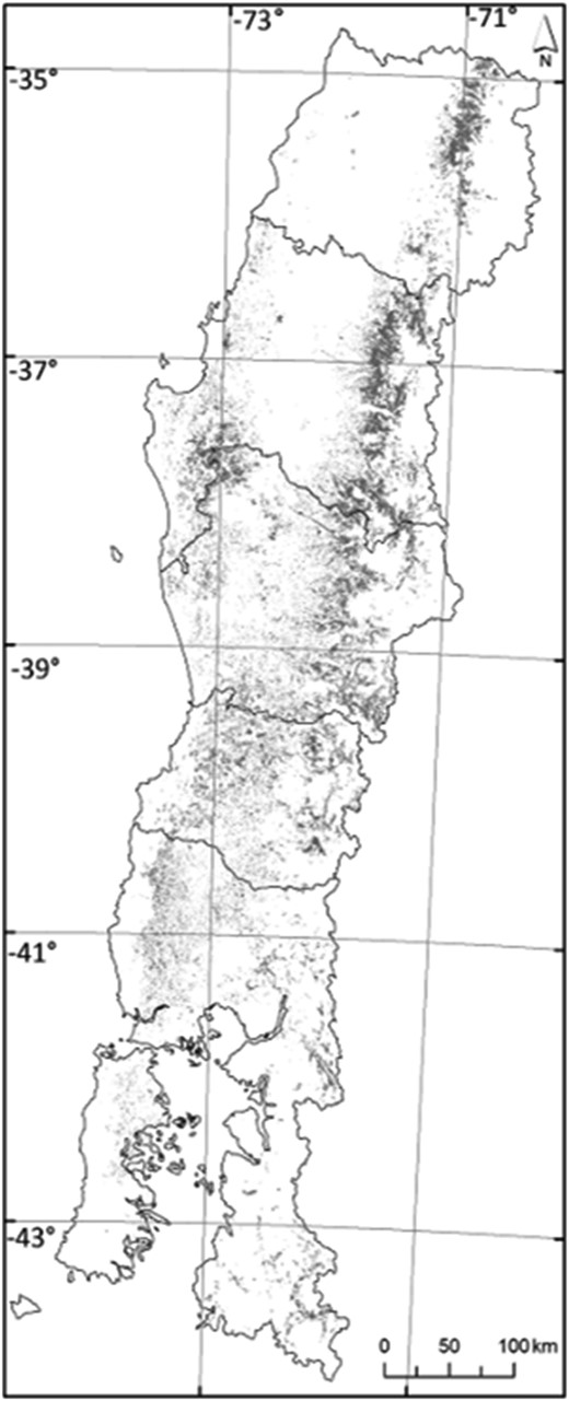
Geographic distribution of the Roble-Rauli-Coihue forest type in Chile.
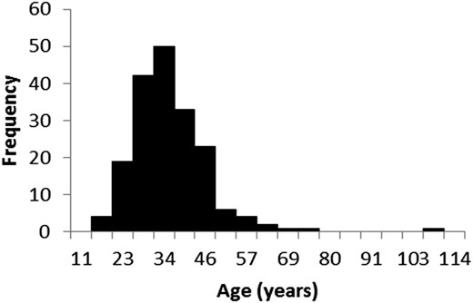
Estimated age distribution of Roble-Rauli-Coihue second-growth forest in Chile.
Data
The data and information considered here are based on the National Forest Inventory (NFI), collected periodically by the Chile Forest Research Institute (Instituto Forestal, INFOR), from 2000 to 2010. The NFI is a permanent sample-based forest inventory that samples forests on all forest site conditions. More than 90 variables are identified and collected from the field and grouped as general variables (e.g. local plot conditions), sample plot variables (e.g. number of trees), tree size attributes (e.g. height, diameter), tree health (scored), soil attributes, regeneration, and vegetation variables (other vegetation on the plot), mortality, and fallen woody debris (INFOR, 2000).
The sampling design applied by the NFI uses a systematic layout of clustered plots from a total number of 1200 permanent sample units. Inverted north-oriented L-shaped transects are placed randomly in stands and located >100 m from any edge. The sampling unit is defined as three 500 m2 circular plots, separated by 110 m along each transect. Each circular sample plot is composed of four area equivalent concentric circular nested subplots. All trees of >4 cm dbh are counted, trees with a dbh of ≤4 cm are measured as regeneration by counting species in each of four height classes. The data are stored in a database (Data Model) and geo-referenced to produce effective and up-to-date information used for any analyses.
Although the RoRaCo forest type is resilient to natural and some harvest disturbances, there are limits to its resilience, as for example through persistent unsustainable harvesting. The identification of possible thresholds was our main interest, given that the current cutting rates are perceived as excessive by some managers. As a tool for identifying a threshold for sustainable versus unsustainable harvesting, we used the relative density concept (Bahamóndez et al., 2010) to distinguish between degraded and non-degraded forest stands from the perspective of expected production. The concept of expected productivity was proposed by Gingrich (1967), pioneered by Reineke (1933) and has been used to aid forest management decisions for many decades (Long et al., 1988; Long and Smith, 1984; Newton, 1988; Chauchard et al., 1999; Woodall et al., 2005, 2006) and persistent change can indicate degradation (Thompson et al., 2013).
Stocking chart
For Chile, the RoRaCo forest type stocking chart was first developed by Gezan et al. (2007) and the current updated version was built by INFOR (2010). The latter version was based on suitably filtered NFI data and is used by the Chilean Forest Service (Corporación Nacional Forestal, CONAF) as a tool to aid forest management. We applied our data on the Gingrich forest stocking chart because we expected that it represented all the possible states of these forests. Without intervention, the trees should follow a continuous process of competition for available light and nutrients as the stand ages (Husch et al., 1982). A stand that is considered ‘overstocked’ has a maximum tree density that grows under strong competition, with consequent high mortality and low annual increments. On the other hand, an ‘understocked’ stand has a low stem density, large annual increments and is below the full productive potential of the site. Managers aim for stem densities between these two extremes to optimize the growth potential for a stand on a given site, over time.
The Gingrich stocking chart deals with forest stocking management decisions and so reflects forest interventions as cutting rates, where these interventions are a discrete process, which is different from natural forest development. The stocking chart represents, for the same time period, the number of trees, tree basal area, tree area ratio and crown competition factors. The data used to generate the stocking chart were derived from forest inventory, specific sampling or other available sample-based data including the NFI data (Figure 3).
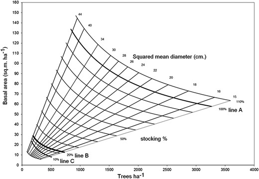
An example of a stocking chart showing the relationship among trees ha−1, basal area ha−1 and percentage of crown canopy.
Interpretation of a stocking chart is as follows: Line-A depicts the fully stocked forest, i.e. areas where trees grow under competition and fully occupy the site capacity. A forest located above Line-A is under strong competition. Line-B depicts the limit where trees can develop large crowns and fully occupy the site capacity but without excessive competition. Finally, Line-C represents the lowest stocking achievable to reach the B-line after a period of 10 years, or any other time period determined by expert consensus, while the straight lines depict the squared mean diameter classes.
Identification of a threshold
Using the Gingrich diagram, Bahamóndez et al. (2010) suggested that all the n-tuples of a forest (basal area/ha, trees/ha) located below Line-C could be considered as degraded, from the forest stocking (or production) perspective. This indicator appears reasonable, and its effectiveness has been successfully tested in the context of forest management (Muller-Using et al., 2012). This framework could provide an early warning indicator that would be valuable for managers to help avoid excessive cutting and enabling forest protection by keeping the stand in a condition away from a threshold. The multiple combinations of n-tuples defined by the stocking chart represents all the possible states that this forest can produce. Under natural development, the forest follows a smooth and almost continuous trajectory of production, mainly dominated by self-thinning as a result of forest aging and competition.
In (2), the expression [1−Pt−1/MAX] is perceived as a density-dependent growth rate modifier, which moves according to the level of the population relative to MAX, allowing for modulation of R values. If Pt−1 →MAX, R decreases, but on the other hand, if Pt−1 → 0, the intrinsic rate of growth may be potentially expressed.
If we observe the relationship between trees ha−1 – basal area ha−1 in the stocking chart, we can identify the space available to grow as the limiting resource and we define the basal area/hectare as the most suitable variable to approach site occupancy. Thus, carrying capacity (MAX) is expressed as a maxima for basal area at a certain stocking level (Figure 4).
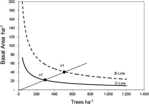
The value for MAX varies according to the level of stocking. In this figure, MAX equals 40 m2 (dot at P1). The forest was taken from P1 to Point P2 (25 m2) by harvesting, where the difference between P1 and P2 represents the energy released from the system providing a space opportunity for the remaining forest to grow and take advantage of the released resources.
The use of the Monod function is central to connecting the stocking chart with the R parameter, because both together enable the use of a logistic discrete function as a means to depict resilience and degradation. Although the dynamics of forest ecosystems are certainly more complex and can be modelled more accurately (e.g. see Botkin 1983; Garcia 1983; Vanclay 1994), the simplicity of the formulations in (1) and (2) can, however, be used to model production trajectories for the purposes of producing objective measurements for growth prediction.
In general, values of R range between 0 and 4 and for the various R values, the discrete logistic function behaves differently (Figures 5 and 6). Based on this behaviour, we associated the pathway from stability, to instability (Figures 5 and 6, respectively), by using the discrete logistic function model. The erratic non-monotonic behaviour of the logistic discrete function (Figure 6) observed when R surpasses a certain threshold value is parameterized here to approach an early warning indicator of forest degradation and loss of resilience.
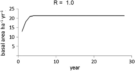
Stand growth under sustainable management.
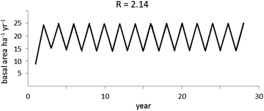
Unpredictable stand growth behaviour suggesting unsustainable management.
Results
Model parameterization
The relationship of the stocking chart and logistic discrete function requires the parameterization of R by applying the expression proposed in [3]. By inspecting the NFI database, we identified the maximal growth rate in basal area (Gmax) as 2.4 m2 ha−1 year−1. The parameter Ks, the basal area at 50 per cent of Gmax, was determined empirically as 11.0 m2 ha−1 year−1, by identifying the removed basal area when R = 1 (Figure 7).
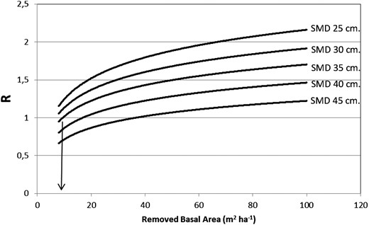
Empirical determination of Ks at Gmax.
From Figure 7, forests with square mean diameter (SMD) values of >35 cm seems to be asymptotically stable, given R < 2.14. That is, even with removal of 125 m2 ha−1, the R values remained below 2.14. On the other hand, forests with an SMD of <35 cm exhibited a limit of potential basal area removal of ∼25, and 65 m2 ha−1, for forests with an SMD = 25 cm, and SMD = 30 cm, respectively.
In Figure 8, each point represents a group of 222 sample plots distributed in stands of the RoRaCo forest type, with different densities (trees ha−1 and basal area ha−1), while the straight lines denote the diameter class guidelines (SMD) and the set of decreasing potential curves represent the stocking (Stock) in relation to full stocking at Line A. Thus, every point represents a vector state (trees ha−1, basal area ha−1, SMD, Stocking). When a forest is managed, interventions force the stand stocking values to move downwards, following a path along these lines and reducing the density within the boundaries defined by Line A of 100 per cent stocking and Line B. From inspection of this chart, it is notable that there are many stands of this forest type located below Line C, which are assumed to be degraded.
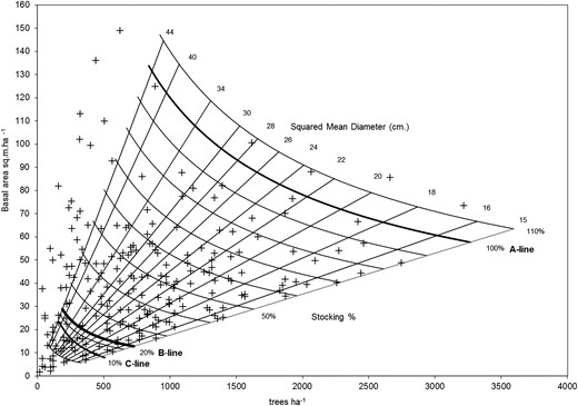
The inventory data from stands of the RoRaCo forest type in Chile plotted on the stocking chart for that forest type. Note the large number of points (i.e. stands) below Line C.
To apply this method, the following example illustrates how degradation and resilience can be determined, using a real forest example: Consider Gmax = 2.4 m2 ha−1
From Figure 8, let us take one point currently below Line C collecting the observed trees ha−1 (T), observed basal area ha−1 (Go), SMD and Stocking level as: T = 141; Go = 13.0 m2 ha−1; SMD = 35.0 cm; Stocking = 10 per cent.
A problem with this forest is that the initial state (in the past) is unknown. Thus, we may apply and test several starting points by moving back by the particular SMD guideline associated with this point (in this case, SMD = 35 cm).
Select arbitrarily from the stocking chart a set of trees ha−1 as Ttheoretic corresponding to the intersection with a specific stocking curve. In this case, intersecting 60, 40, 20 and 10 per cent stocking lines.
- Calculate the theoretical basal area when trees ha−1 equal Ttheoretic by using the general expression (4) of stocking lines, notice when the stocking (Stock) is 1.0 (100 per cent), referring to full stocking, i.e. Line-A:where Gha is the theoretical basal area ha−1 (m2 ha−1) for Ttheoretic trees ha−1 Stock is stocking level [0;1] K = 8920.0 Ttheoretic is trees ha−1.(4)
Estimate Grmn = Gha − Go
Estimate R according to expression (3)
In this case, we tested for the following starting points, targeting 141 trees ha−1 and 13.0 m2 ha−1, 10 per cent stocking. These calculations produced the results shown in Table 1.
Using the estimated R values, expression (2) allows for examination of stability, in this case within a 10-year period (Table 2).
Results from Step 7 (see text) for R using a target of 141 trees ha−1 and 13.0 m2 ha−1, with 10% stocking
| Stocking | 60% | 40% | 20% | 10% |
|---|---|---|---|---|
| Trees ha−1 | 826 | 526 | 342 | 201 |
| Theoretical basal area (m2ha−1) | 82.6 | 72.9 | 47.6 | 33.1 |
| Gc (m2 ha−1) | 69.6 | 59.9 | 34.6 | 20.1 |
| R | 2.07 | 2.03 | 1.82 | 1.55 |
| Stocking | 60% | 40% | 20% | 10% |
|---|---|---|---|---|
| Trees ha−1 | 826 | 526 | 342 | 201 |
| Theoretical basal area (m2ha−1) | 82.6 | 72.9 | 47.6 | 33.1 |
| Gc (m2 ha−1) | 69.6 | 59.9 | 34.6 | 20.1 |
| R | 2.07 | 2.03 | 1.82 | 1.55 |
Inspecting the logistic discrete behaviour, an example
| Time (year) | Pt60% (m2 ha−1) | Pt40% (m2 ha−1) | Pt20% (m2 ha−1) | Pt10% (m2 ha−1) |
|---|---|---|---|---|
| 1 | 13.00 | 13.00 | 13.00 | 13.00 |
| 2 | 35.7 | 34.66 | 30.21 | 25.25 |
| 3 | 77.72 | 71.52 | 50.33 | 34.56 |
| 4 | 87.27 | 74.25 | 45.11 | 32.23 |
| 5 | 77.09 | 71.44 | 49.43 | 33.57 |
| 6 | 87.78 | 74.32 | 46.00 | 32.86 |
| 7 | 76.41 | 71.37 | 48.85 | 33.26 |
| 8 | 88.31 | 74.4 | 46.55 | 33.04 |
| 9 | 75.70 | 71.29 | 48.45 | 33.16 |
| 10 | 88.83 | 74.48 | 46.91 | 33.10 |
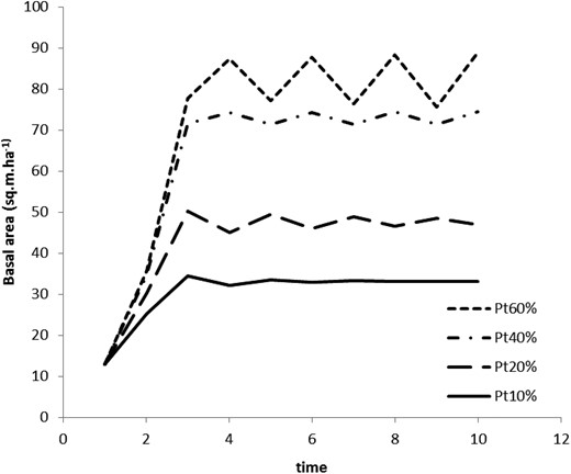
An example of the logistic discrete modelled behaviour of stand growth over time. The small-dashed trajectory indicates instability with R = 2.07, the mixed dash-dotted curve describes an initial state of instability with R = 2.01, while the long-dashed (R = 1.82) and solid (R = 1.55) trajectories are stable conditions for the RoRaCo forest type.
Forest growth becomes highly unstable when the logging intervention is too intensive and rapidly reaches levels near Line C. The stand is stable within the area determined by Line A (100 per cent stocking) and Line B (Figures 5 and 6), suggesting this method would be a useful tool for depicting resilience capacity.
To produce a visual representation of resilience, following Walker et al. (2004), we used a three-dimensional representation as a stability landscape map. This tool allowed us to approach and describe instability. The landscape stability map was produced by plotting the rates xt vs (1−xt) from expression [1]. The values of xt in this context are interpreted as the resultant rate after the intrinsic growth is modified by the resources dependent rates (1−xt). At the moment of cutting, xt and (1−xt) share a stable combination of values where xt + (1−xt) = 1.0. Once cutting is completed, this balance is lost and xt + (1−xt) < 1.0 for a period of time, until the balance returns. Figure 10 illustrates this effect as a three-dimensional landscape stability map for the cases for Pt10% and Pt60% from Table 1.
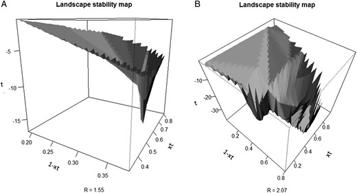
(A) An example of a landscape stability map for R = 1.55 and (B) a landscape stability map for R = 2.07. The inverted peak for R = 1.55 represents the expected stable values (xt = 0.35, (1−xt) = 0.65) for the stand to return to the original condition after cutting has been performed. When R = 2.07, there is no one single peak and the system shows instability.
We have used diagrams similar to Beisner et al. (2003) to illustrate the variance of ecosystem conditions and basins that attract the system back towards a stable state, or inverted basins that illustrate unpredictable change to another ecosystem state. These basins represent the successional trajectories of a forest stand following harvesting. In our case, these diagrams were quantified along three axes, xt rate at time t on the X axis, (1−xt) rate at time t on the Y axis, and time corresponds to the Z axis, rather than simply being heuristic. The surface roughly indicates the path close to original state or, to new states with different levels of stability.
In Figure 10 right, the forest, when forced into a region of instability by excessive harvesting, takes a position close to the peak of the surface and, as a consequence, the system responds with multiple possible domains (i.e. ecosystem states), where none is predominant or predictable. That is, the threshold value for resilience in this ecosystem (Figure 10 right) was surpassed resulting in a precarious condition and indicating that this forest was unsustainably managed. Among the stands of RoRaCo in Chile, close to 17 per cent (ca. 170 000 ha) are considered degraded given their position below Line C (Figure 8), which denotes a post-cutting situation with abnormal vertical structure dominated by a few large trees, with open areas completely covered by native invasive bamboo species Chusquea coleu Devaux and Chusquea quila Kunth. On the other hand, a well-managed forest (Figure 10 left) presents a much different stability landscape, where a distinctive domain, or attractor, forces the recovering stand towards a single steady state. This state has a high resilience, forcing the temporary new state that follows management to be attracted back to the dominant state (illustrated as the inverted peak or basin). Typically, a stable well-managed forest is characterized by a normal tree diameter distribution, occurring above Line B (Figure 8) and is not invaded by bamboos. Hence, the hysteresis of the forest state in Figures 10 left and right are clearly different.
From Figure 4, the most resilient RoRaCo forests are those with an SMD > 35 cm, given the possible values of R that exceed the level resulting in values that range from weak to transitional resilience to loss of resilience. The most vulnerable stands, then, would be in SMD classes <35 cm. The path of degradation, or the gradual transition from a stable state towards an unstable state, is illustrated in Figure 11, as an example of the trend shown by a sequential series of landscape stability maps along the various values of R, when the forest moves from a stable to an unstable condition. Box 1 (Figure 11) illustrates a well-managed harvested forest, where the long pronounced inverted peak denotes a strong dominant force (attractor) towards a stable condition. Boxes 2 and 3 show the transition towards instability, characterized by the inverted peak to flatness. Boxes 4–6 illustrate multiple possible inverted peaks and suggest that resilience is gradually lost with increased levels of harvesting.
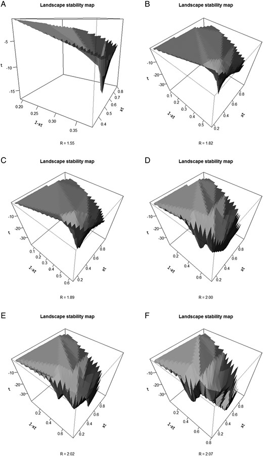
Sequential development of instability illustrating sustainable to unsustainable forest management. This sequence shows the path toward instability, (A) represents the full stable condition, while (F) represents a highly unstable condition.
Discussion
We have presented a method to quantify and predict forest degradation and resilience from a production perspective, including thresholds and illustrating the loss of resilience in a specific forest ecosystem, using common forest inventory data. One of the key elements in forecasting a possible path towards forest degradation is represented by the parameter R in (1), (2) and (3). R, in the context of population dynamics, represents a rate of growth when the initial population is small compared with a pre-defined maxima or, as a rate of reduction when a population is close to the maxima. In order to discriminate between these dual behaviours, R is empirically defined by a Monod function allowing it to match the logistic discrete value with the stocking chart. Originally, the Monod equation, and other similar equations (e.g. Michaelis–Menten), explain R as a maximal growth rate (Gmax) weighted by an asymptotic proportion of added woody biomass in the system. Here, instead of adding woody biomass to the system, biomass is lost by removing basal area through harvesting, thinning, or natural mortality. Given those processes, and to adjust R values to match those of the stocking chart, Gmax was specified to values found after inspecting the NFI database for all SMD classes. It is important to recognize that the greater the basal area removed and the shorter the return time, the higher the probability of degrading the forest, especially when cutting forces the forest to a condition under the line C. The path to degradation would eventually also represent a loss of resilience in the system, given the trends shown by resilience attributes including latitude and precariousness (Walker et al., 2004).
Identifying tipping points is often problematic but our results suggested that forest productivity, measured in terms of stand growth, can readily be used to suggest a threshold that can be used to inform management. Furthermore, the method that we have applied makes use of standard forest inventory data from permanent sample plots over time and so is applicable in any managed forest type for which similar forest inventory data are available. Our result for this forest type, that excessive cutting of trees <35 cm diameter SMD increases instability, is consistent with empirical and published evidence that old forests of many types are more resilient than young forests to disturbances (Luo and Chen, 2013). The prediction of tipping points is important if forests are to be managed sustainably.
Our results highlight the value of a stand stocking chart as a powerful tool to advance the assessment of forest stability and resilience in self-replacing forests. Our analysis showed that resilience will be protected if harvesting levels in this Nothofagus forest example occur within the limits defined between Lines A and B, and disturbances do not force the system below Line C. Our proposed approach enables forest practitioners to better understand the effects of management prescriptions on forest stability and provides a reasonably simple method to enable managers to avoid tipping points. This approach affords an opportunity to observe, with real data, and to graphically illustrate the pathways for a stand, defined through management prescriptions and enabling the determination of tipping points, while observing resilience attributes operationally, rather than suggesting them in theory only.
Forest degradation can have many causes that are often linked in a synergistic fashion (Chazdon 2008), for example logging followed by fire (Asner et al., 2006). Certainly, our forest type in Chile, RoRaCo, suffers annual depletions from various natural sources such as windthrow and diseases. Forest managers and management models need to be cognizant of and account for depletions from these multiple sources and attribute basal area loss accordingly. Further, given current environmental changes, it is important for managers to consider managing towards adaptive capacity rather than sustained yield (Messier et al., 2013). Here, we have presented data to illustrate degradation with respect to production, which represents one type of forest degradation. It is important to recall, however, that forests can undergo other forms of degradation as well, including through the loss of biodiversity, loss of carbon storage capacity, loss of protective functions, and as a result of multiple unusual disturbances, all of which result in reduced goods and services (Thompson et al., 2013). We see the quantified approach used here as a way to provide practitioners with, in part, a systems ecology understanding of a transition from a sustained yield standard to ecosystem management with an ultimate objective of gradually providing a pathway towards adaptive management of complex systems while avoiding forest degradation (Filotas et al., 2014).
Conflict of interest statement
None declared.
