Global 3-D EM inversion of Sq variations based on simultaneous source and conductivity determination: concept validation and resolution studies

Abstract

We present a novel global 3-D electromagnetic (EM) inverse solution that allows to work in a unified and consistent manner with frequency-domain data that originate from ionospheric and magnetospheric sources irrespective of their spatial complexity. The main idea behind the approach is simultaneous determination of the source and conductivity distribution in the Earth. Such a determination is implemented in our solution as a looped sequential procedure that involves two steps: (1) determination of the source using a fixed 3-D conductivity model and (2) recovery of a 3-D conductivity model using a fixed source. We focus in this paper on analysis of Sq data and numerically verify each step separately and combined using data synthesized from 3-D models of the Earth induced by a realistic Sq source. To determine the source we implement an approach that makes use of a known conductivity structure of the Earth with non-uniform oceans. Based on model studies we show that this approach outperforms the conventional potential method. As for recovery of 3-D conductivity in the mantle, our inverse scheme relies on a regularized least-square formulation, exploits a limited-memory quasi-Newton optimization method and makes use of the adjoint source approach to calculate efficiently the misfit gradient. We perform resolution studies with checkerboard conductivity structures at depths between 10 and 1600 km for different inverse setups and conclude from these studies that: (1) inverting Z component gives much better results than inverting all (X, Y and Z) components; (2) data from the Sq source allows for resolving 3-D structures in depth range between 100 and 520 km; (3) the best resolution is achieved in the depth range of 100–250 km.

Numerical solutions, Inverse theory, Geomagnetic induction

1 INTRODUCTION

Understanding 3-D physical properties of the Earth's mantle is one of the challenging tasks of modern geophysics. Estimates of 3-D variations of the Earth's properties come mainly from global seismic tomography (Becker & Boschi 2002; Panning & Romanowicz 2006; Kustowski et al.2008, among others). While substantial progress in seismology models has been achieved recently, the interpretation of the seismic velocity anomalies in terms of thermo-dynamical and compositional parameters is often uncertain and needs additional information (e.g. Trampert et al.2004; Khan et al.2009). A complementary means to directly probe physical properties of the mantle is deep electromagnetic (EM) induction sounding, which can potentially recover—from predominantly magnetic field variations continuously recorded at a worldwide network of geomagnetic observatories—the 3-D electrical conductivity distribution in the Earth's mantle. To separate the effects of composition and temperature, or to illuminate the role of partial melt and fluids (especially water) in the mantle, both seismic and EM techniques are likely to be important (Khan & Shankland 2012).

Regarding the EM technique, it is pertinent to emphasize that it is only through recent improvements in global 3-D EM forward modelling and growth of computational resources that full 3-D EM inversion on a global scale has become feasible. A few inverse 3-D solutions have been developed recently (Koyama 2001; Kelbert et al.2008; Tarits & Mandea 2010; Kuvshinov & Semenov 2012), providing the first semi-global (Fukao et al.2004; Koyama et al.2006; Utada et al.2009; Shimizu et al.2010) and global (Kelbert et al.2009; Tarits & Mandea 2010; Semenov & Kuvshinov 2012) 3-D mantle conductivity models. Recent progress in global 3-D forward and inverse modelling is summarized in the review papers by Kuvshinov (2008, 2012).

All aforementioned studies use disturbed stormtime variations (D_st) originating from the magnetospheric ring current. Moreover in most of the studies (except for the work of Tarits & Mandea 2010) the dipolar characteristics of this current are assumed, that is, the source magnetic potential is described by a first zonal spherical harmonic in the geomagnetic coordinate system. There is a common consensus that this assumption is valid for the signals in a period range between a few days and a few months and thus allows the use of the local C-response concept (e.g. Banks 1969). The complex-valued C-response has physical dimension of length and its real part provides an estimation of the depth to which the EM field penetrates (Weidelt 1972). Bearing in mind the considered period range, a 3-D interpretation of local C-responses conducted in the studies cited allows for the recovery of electrical conductivity in the depth range from about 400 km down to 1500 km.

However there is great interest in mapping electrical conductivity at upper-mantle (UM) depths (100–400 km). Recent laboratory experiments demonstrate that the electrical conductivity of UM minerals is greatly affected by small amounts of water or by partial melt (Wang et al.2006; Gaillard et al.2008; Yoshino et al.2009, among others). Determination of UM conductivity using EM methods can thus provide constraints on melting processes and the presence of water in the upper mantle. Probing conductivity at UM depths requires EM variations in a period range between a few hours and 1 d. This is a challenging period range for global EM studies since the ionospheric (Sq) source, which dominates this period range, has a much more complex spatial structure compared to the magnetospheric D_st source. The interested reader is referred to the publications of Parkinson (1977), Winch (1981) and Schmucker (1999a,b) where the spatial structure of the Sq current system is discussed. In addition, the complexity of the Sq source rules out the possibility of using the local C-response concept. Note that this period range is also challenging for magnetotelluric (MT) methods (Shimizu et al.2011), since for these periods the Sq source strongly affects the MT signals, which are assumed to originate from a vertically propagating plane-wave source.

In this paper we present a novel global 3-D inverse solution that allows us to work in a unified and consistent manner with frequency-domain EM data that originate from both, ionospheric and magnetospheric, sources irrespective of their spatial complexity. The solution relies on an approach proposed by Fainberg et al. (1990) and applied so far to the 1-D inversion of D_st data (Singer et al.1993). The two key ideas behind this concept are: (1) one has to work with the fields (more exactly with the time spectra of the fields) rather than with the responses and (2) one has to determine simultaneously the parameters describing the source and conductivity distribution in the Earth. The simultaneous determination of the source and conductivity is implemented in our solution as a looped sequential procedure that involves two steps: determination of the source using a fixed 3-D conductivity model and recovery of a 3-D conductivity model using a fixed source (Fig. 1). We remark here that we concentrate in this paper on a discussion of this approach as applied to data from the complex Sq source. As far as we know, there have been no attempts to invert Sq data (either synthetic or observed) in the frame of 3-D conductivity models of the Earth. The paper is organized as follows. In Section 2 we present an approach for the source determination, which makes use of the Earth's known conductivity structure (hereinafter we call this approach the S3D method). We also recapitulate the potential method in this section and carried out model studies—using a realistic 3-D earth model and a realistic Sq source—to compare the performance of the two methods. In Section 3 we introduce and verify the 3-D inverse scheme to recover the 3-D conductivity distribution in the mantle from Sq data with the assumption that the Sq source is known (fixed). Our inverse scheme to recover the conductivity distribution closely follows an inverse scheme described in Kuvshinov & Semenov (2012). It is based on a regularized least-squares formulation, exploits a limited-memory quasi-Newton optimization method and makes use of the adjoint source approach to calculate efficiently the misfit function gradient. Since the new approach presented here works with the time spectra of the magnetic field instead of the C-responses, modification of the misfit gradient calculations were required by elaborating a new adjoint source. This has been done using the formalism developed in Pankratov & Kuvshinov (2010). As a forward problem engine to calculate EM fields an integral equation (IE) solver (Kuvshinov et al.2002; Kuvshinov 2008) is invoked. In Section 4 we perform resolution studies using checkerboard multilayered 3-D models and various inverse problem setups. In Section 5 we verify the overall scheme (which is summarized in Fig. 1) using the numerical solutions developed in Sections 2–4. Section 6 contains conclusions and Section 7 suggests topics for the future work.

Figure 1.

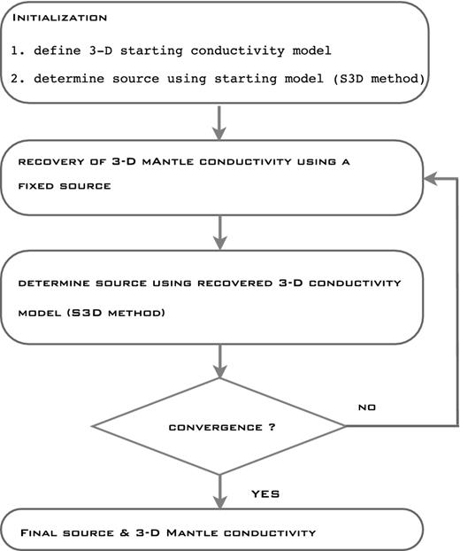
Looped sequential solution scheme to the problem of global inversion of ground-based EM data. The scheme involves two steps. Step 1: recovery of a 3-D conductivity model using a fixed source; Step 2: determination of the source using a fixed 3-D conductivity model.

2 SOURCE DETERMINATION

The accurate determination of the source is a necessary prerequisite for rigorous 3-D inversion of Sq global induction data. Recognizing that the source description can be done using different spatial forms, we rely in this paper on an expansion of the source utilizing spherical harmonics (SH). Derivation of the external SH coefficients that describe the source is presented employing two approaches. The first approach exploits the standard potential method (Gauss 1839), the second—S3D—makes use of the Earth's known conductivity structure. We carried out model studies on synthetic but realistic Sq data to compare the performances of the two methods.

2.1 Potential method

We start by writing Maxwell's equations in the frequency domain

\begin{equation} \frac{1}{\mu _0}\nabla \times \mathbf {B}(\mathbf {r})=\sigma (\mathbf {r})\mathbf {E}(\mathbf {r})+\mathbf {j}^{\rm ext}(\mathbf {r}), \end{equation}

(1)

\begin{equation} \nabla \times \mathbf {E}(\mathbf {r})={\rm i}\omega \mathbf {B}(\mathbf {r}), \end{equation}

(2)

assuming that displacement current effects are negligible in the considered period range. B(r), E(r) and σ(r) are the magnetic field, electric field and conductivity distributions, respectively, r = (r, θ, ϕ), where r, θ and ϕ designate spherical radius, co-latitude and longitude, respectively. Further, μ_o designates the magnetic permeability of free space, and j^ext stands for an impressed (extraneous) current. Note that dependence of B, E and j^ext on the angular frequency ω is omitted but implied. We adopt the Fourier convention

\begin{equation} f(t) = \frac{1}{2\pi }\int _{-\infty }^{\infty } f(\omega ){\rm e}^{-{\rm i}\omega t} {\rm d}w. \end{equation}

(3)

Above the Earth's surface (in an insulating atmosphere) and outside the source, eq. (1) reduces to

\begin{equation} \nabla \times \mathbf {B}=0, \end{equation}

(4)

allowing the derivation of the magnetic field B in this region from the magnetic potential V

\begin{equation} \mathbf {B}=-\nabla V. \end{equation}

(5)

By using the solenoidal property of the magnetic field

\begin{equation} \nabla \cdot \mathbf {B}=0, \end{equation}

(6)

potential V satisfies Laplace's equation

\begin{equation} \Delta V=0, \end{equation}

(7)

whose general solution can be represented as a sum of external and internal parts

\begin{equation} V=V^{\rm ext}+V^{\rm int}, \end{equation}

(8)

where the external and internal parts in spherical coordinates are given by

\begin{equation} V^{\rm ext}(\omega ,r,\theta ,\phi )=a\sum \limits _{n=1}^{\infty }\sum \limits _{m=-n}^{n}\epsilon _n^m(\omega )\left(\frac{r}{a}\right)^{n}Y_n^m(\theta ,\phi ), \end{equation}

(9)

\begin{equation} V^{\rm int}(\omega ,r,\theta ,\phi )=a\sum \limits _{n=1}^{\infty }\sum \limits _{m=-n}^{n}\iota _n^m(\omega )\left(\frac{a}{r}\right)^{n+1}Y_n^m(\theta ,\phi ). \end{equation}

(10)

Here a is a mean radius of the Earth, |$\epsilon _n^m$| and |$\iota _n^m$| are complex-valued functions of ω, and the SHs are

\begin{equation} Y_n^{m}(\theta ,\phi )= P_n^{|m|}(\cos \theta )e^{im\phi }, \end{equation}

(11)

where |$P_n^{|m|}$| are Schmidt quasi-normalized associated Legendre polynomials. Using eqs (5) and (8) we can write the magnetic field B in the form

\begin{equation} \mathbf {B}=\mathbf {B}^{\rm ext}+\mathbf {B}^{\rm int}, \end{equation}

(12)

where

\begin{equation} \mathbf {B}^{\rm ext}=-\nabla V^{\rm ext}, \end{equation}

(13)

\begin{equation} \mathbf {B}^{\rm int}=-\nabla V^{\rm int}. \end{equation}

(14)

Using eqs (12)–(14) and eqs (9) and (10) one can obtain the representation of the geomagnetic field components B_r, B_θ and B_ϕ above the Earth as functions of r, θ, ϕ and ω. By equating r to a one writes the expressions for the field components at a ground-based observatory j as

\begin{equation} B_r^{\rm exp}(\omega ,a,\theta _j,\phi _j)= - \sum \limits _{n,m} [n \epsilon _n^m(\omega ) -(n+1) \iota _n^m(\omega ) ] Y_n^m, \end{equation}

(15)

\begin{equation} B_\theta ^{\rm exp}(\omega ,a,\theta _j,\phi _j)= -\sum \limits _{n,m} [ \epsilon _n^m(\omega ) + \iota _n^m(\omega ) ]\frac{{\rm d}Y_n^m}{{\rm d}\theta }, \end{equation}

(16)

\begin{equation} B_\phi ^{\rm exp}(\omega ,a,\theta _j,\phi _j)= -\sum \limits _{n,m} [ \epsilon _n^m(\omega ) + \iota _n^m(\omega ) ]\frac{im}{\sin \theta } Y_n^m, \end{equation}

(17)

where ∑_{n, m} is a short expression for the double sums in eqs (9) and (10) and superscript exp stands for the experimental data from geomagnetic observatories. We can now estimate the external (inducing) coefficients |$\epsilon _n^m(\omega )$| (which describe the source) and the internal (induced) coefficients |$\iota _n^m(\omega )$| by least-squares fitting to the available data from the global net of geomagnetic observatories using the linear system of eqs (15)–(17).

2.1.1 Discussion of the method

By using the potential method one is not confined to the use of all components (B_r, B_θ, B_ϕ) but can also use combinations of only one horizontal component and the radial component (but we note that B_r is obligatory to include in the analysis). Furthermore, the potential method provides a solution without any knowledge of the underlying conductivity structure and in addition to the external (inducing) SH coefficients one gets the internal (induced) SH coefficients.

If the distribution of observations is regular and dense over the globe, the potential method provides adequate separation of external and internal coefficients irrespective of whether the Earth is characterized by 3- or 1-D conductivity distributions. In this case only the density of observations becomes the factor that limits the highest degree n and order m in the expansion of either inducing and/or induced parts of the potential. Note that if the Earth is described by a radially symmetric (1-D) conductivity distribution [i.e. σ ≡ σ(r)], each external coefficient induces only one internal coefficient (of the same degree n and order m). In the general case of a 3-D conductivity structure, that is, σ ≡ σ(r, θ, ϕ), each external coefficient induces a whole spectrum of internal coefficients.

However, in reality ground-based geomagnetic observatory data are very sparsely and irregularly distributed over the globe. Only a few observatories are located in oceanic regions, while there is an overall deficiency of geomagnetic observatories in the southern hemisphere. Bearing this in mind, one is able to recover only low-order coefficients both in the inducing and induced parts with the potential method. However, in the considered period range one cannot describe the induced radial magnetic field by a low-order expansion, since this component (at least at coastal and island observatories) is dramatically affected by the 3-D ocean effect, which requires higher SH for its proper description [see examples of the ocean effect both in observations and predictions in Kuvshinov (2008)]. In the next section we discuss a method which overcomes this problem.

2.2 S3D method

The S3D method is based on a numerical solution of Maxwell's equations in a spherical 3-D earth model that accounts for the ocean effect. Since the ocean effect arises because of a non-uniform distribution of highly conducting oceans and highly resistive continents, it can be represented in the model by a thin surface layer of fixed laterally variable conductance, which, in turn, is (mostly) governed by the known bathymetry of the oceans. This layer can be underlain by either a 1- or 3-D conducting mantle. What follows is a sketch of the S3D method. We first introduce the extraneous current j^ext in eq. (1) using

\begin{equation} \mathbf {j}^{\rm ext}=\frac{\delta (r-b)}{\mu _0} \sum _{n,m} \frac{2n+1}{n+1}\epsilon _n^m(\omega )\left(\frac{b}{a}\right)^{n-1} \mathbf {e}_r\times \nabla _{\bot } Y_n^m, \end{equation}

(18)

with

\begin{equation} \nabla _{\bot } Y_n^m=\mathbf {e}_{\theta } \frac{ \partial Y_n^m}{ \partial \theta } + \mathbf {e}_{\phi } \frac{1}{\sin \theta } \frac{\partial Y_n^m}{ \partial \phi }, \end{equation}

(19)

where δ denotes Dirac's delta function, e_r, e_θ and e_ϕ are unit vectors of the spherical coordinate system, and × denotes a vector (cross) product. The extraneous current j^ext flows in a thin shell at r = b ≥ a and produces exactly the external magnetic field B^ext in the region a ≤ r < b [see appendix G of Kuvshinov & Semenov (2012) for details]. By letting b = a we represent j^ext as

\begin{equation} \mathbf {j}^{\rm ext}= \sum \limits _{n,m}\epsilon _n^m(\omega )\mathbf {j}_n^{m, {\rm unit}}, \end{equation}

(20)

with

\begin{equation} \mathbf {j}_n^{m, {\rm unit}}=\frac{\delta (r-a)}{\mu _0} \frac{2n+1}{n+1} \mathbf {e}_r\times \nabla _{\bot } Y_n^m. \end{equation}

(21)

By solving Maxwell's equations for each |$\mathbf {j}_n^{m, {\rm unit}}$|

\begin{equation} \frac{1}{\mu _{0}} \nabla \times \mathbf {B}_{n}^{m,{\rm unit}}=\sigma \mathbf {E}_n^{m}+\mathbf {j}_n^{m,{\rm unit}}, \end{equation}

(22)

\begin{equation} \nabla \times \mathbf {E}_n^{m,{\rm unit}}=i\omega \mathbf {B}_n^{m,{\rm unit}}, \end{equation}

(23)

and exploiting the linearity of Maxwell's equation with respect to the source, we can represent (with the use of eq. 20) the geomagnetic field components at a ground-based observatory j as the sum of ‘unit’ magnetic fields |$\mathbf {B}_n^{m,{\rm unit}}$| scaled by the external coefficients |$\epsilon _n^m$|⁠, which we want to determine:

\begin{equation} \mathbf {B}^{\rm exp}(\omega ,a,\theta _j,\phi _j) =\sum \limits _{n,m}\epsilon _n^m(\omega )\mathbf {B}_{n}^{m,{\rm unit}}(\omega ,a,\theta _j,\phi _j). \end{equation}

(24)

By analogy with the potential method we can estimate the external coefficients |$\epsilon _n^m(\omega )$| by least-squares fitting the available data from the global net of observatories using the system of eq. (24). Note that |$\mathbf {B}_n^{m,{\rm unit}}$| is composed of the external field with spherical harmonic mode (n, m) and the field induced in 3-D conductivity earth's model, and thus |$\mathbf {B}_n^{m,{\rm unit}}$| contains all spherical harmonic modes originated from the induced field.

2.2.1 Discussion of the method

An important advantage of the S3D method compared with the potential method is that S3D allows us to include sea-bottom data in the analysis. This is not possible with the potential method, since the sea-bottom observations are performed within a conductor where the potential representation of the magnetic field in the form of eq. (5) is no longer valid. The modification of the S3D scheme is straightforward in this case. One just has to add the equations that relate the experimental and modelled magnetic fields at the sea-bottom

\begin{equation} {\mathbf {B}}^{\rm exp}(\omega ,c_k,\theta _k,\phi _k) =\sum \limits _{n,m}\epsilon _n^m(\omega ){\mathbf {B}}_{n}^{m,{\rm unit}}(\omega ,c_k, \theta _k,\phi _k), \end{equation}

(25)

to the discussed linear system (24) with c_k, θ_k and ϕ_k standing for the coordinates of the k-th sea-bottom site.

Moreover, one can easily incorporate electric field data into the S3D scheme, if such data are available. Again this is not possible with the potential method, even at the surface of the Earth, since the time-varying electric field is not a potential field anywhere. In this case one adds the equations, which relate the experimental and modelled electric fields

\begin{equation} {\mathbf {E}}^{\rm exp}(\omega ,d_i,\theta _i,\phi _i) =\sum \limits _{n,m}\epsilon _n^m(\omega ){\mathbf {E}}_{n}^{m,{\rm unit}}(\omega ,d_i, \theta _i,\phi _i), \end{equation}

(26)

to the linear system, with d_i, θ_i and ϕ_i standing for the coordinates of the i-th site where the electric field is available. Note also that, contrary to the potential method, we are free to choose any combination of components or even only one of them to estimate |$\epsilon _n^m$|⁠.

One can argue that the results of the S3D method are influenced by the choice of a specific conductivity model of the Earth, which, |$\it a \ priori$| is not known. We would like to argue though, that we are rather safe in the description of the uppermost part of the model (surface shell of fixed conductance), which is governed by a well-established bathymetry. However, a choice of the mantle conductivity structure underneath may indeed influence the source determination, if one considers the S3D method out of the context of mantle conductivity recovery. Once we formulate the problem as a simultaneous determination of the source and the conductivity (as explained in the Introduction and applied in this paper) this is no longer an issue.

The final remark of this section concerns the parametrization of the source. In this paper—since we deal with Sq signals—we parametrize the source by SH (further reasoning for this choice will be presented in the next section). However, within the S3D method we are free to consider any other spatial basis forms, which might prove more appropriate to describe a source.

2.3 Model studies: S3D versus potential method

In this section we perform model studies to compare the actual performance of the potential and the S3D methods as applied to synthetic but realistic Sq data. Before explaining the setup for these model studies we first remind the reader of some facts about the spatio-temporal structure of the Sq current system.

There is a common consensus that the Sq current system is flowing at 110 km altitude in a thin ionospheric E-layer. This current system is driven by atmospheric tides in the ambient magnetic field of the Earth [the interested reader can find more details about the physics behind this current system in the publications of Campbell (1989), Olsen (1997) and Richmond (1995)]. These tides are generated from solar heating of the atmosphere on the sunlit side of the Earth. The Sq current system has a double vortex structure with an anticlockwise (clockwise) whorl in the northern (southern) hemisphere and is bounded between ±6° and ±60° geomagnetic latitude with the whorl centres at around ±35° geomagnetic latitude. It is stationary in the Earth–Sun line due to its solar origin with the Earth rotating underneath it and is observed as a local time (LT) phenomenon. The simplest and the most symmetric structure (with respect to hemisphere balance) of the Sq current system is observed during the geomagnetically quiet days of equinoctial months. In the remainder of this paper all the results correspond to such a day, namely, March 19 of the International Quiet Solar Year (IQSY; 1965).

To represent the Sq current system we follow the approach described in Schmucker (1999a). It is based on a spherical harmonic analysis (SHA) of Fourier-transformed observatory data. According to Schmucker's study, six time-harmonics (p = 1, 2, …, 6) are sufficient to describe a geomagnetic quiet day with 24 hourly values. The summation of SH terms is reversed and controlled by the time harmonic p. The external part of potential V at the surface of the Earth (r = a) is then rewritten in the form

\begin{equation} V^{\rm ext}(a,\theta ,\phi ,\omega _p)= a \sum _{m=p-L}^{p+L}\sum _{n=|m|}^{|m|+K-1} \epsilon _n^m(\omega _p) Y_n^{m,p}, \end{equation}

(27)

where

\begin{equation} Y_n^{m,p}(\theta ,\phi )= P_n^{|m|}(\cos \theta ){\rm e}^{{\rm i}(m-p)\phi }, \end{equation}

(28)

and

\begin{equation} \omega _p=\frac{2\pi }{T}p, \end{equation}

(29)

with T = 24 hr. Following the studies of Schmucker (1999a) on an optimal subset, we choose the series parameter L to be 1 and K to be 4, which results in a subset of 11 coefficients for the first time harmonic (p = 1) and 12 coefficients for all other time harmonics (p = 2, 3, …, 6). The reason for this choice is the 24 hr periodicity of Sq signals and the actual geometry of the Sq source as described in the beginning of this section. As in Schmucker (1999a) we introduce terms where m = p are ‘LT terms’ and m ≠ p are ‘general terms’. The ‘LT terms’ represent the part of Sq which travels westwards with the speed of the sun (15° in longitude per hour). For an observer outside the rotating Earth, Sq appears to be fixed in the Earth–Sun line, consequently the dependence on longitude in eq. (28) vanishes. Within the set of ‘LT terms’ the term of degree n = p + 1 is the largest and most stable term, henceforth denoted as ‘dominating term’. The ‘general terms’ represent the parts of Sq that are not moving westwards with the speed of the Sun. Here m > p represents the part which is traveling faster and 0 < m < p the part which is traveling more slowly than the Sun.

A further decision concerns the choice of the coordinate system. Here we again follow Schmucker's paper, in which he wrote: ‘Since the Sun is the prime cause, geographical coordinates are a natural choice. However, the asymmetry of the Earth's permanent field with respect to the axis of rotation provides an argument for the use of geomagnetic coordinates because this field is responsible for the electromotive driving force of external source currents and also for the directional dependence of ionospheric conductivity. Tests have shown, however, that the choice of coordinates has only marginal influence on the fit by SH.’ Thus we adhere in this paper to the geographic coordinate system.

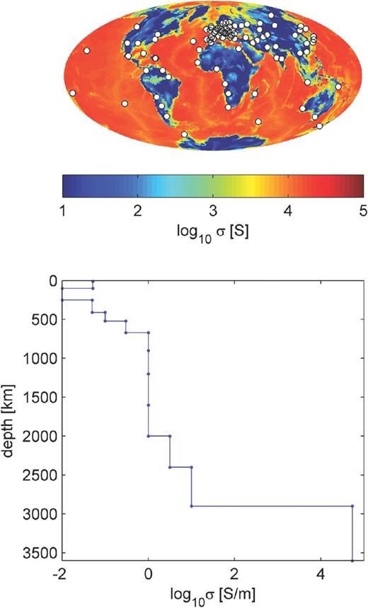
To create a Sq source we analyse real data from 80 mid-latitude observatories for the aforementioned day (19.03.1965). Here mid-latitude observatories stand for observatories between +6° and +60°, and −6° and −60° geomagnetic latitude. This choice is driven by the intention to exclude distorting effects from the equatorial and polar electrojets on the data. The locations of observatories are shown in the upper plot of Fig. 2, whereas their acronyms are presented in Table 1. The potential method and the SH subset from eq. (27) were used to estimate external coefficients, |$\epsilon _n^m(\omega _p)$|⁠, from these data. We used an iteratively re-weighted least square (IRLS) algorithm (e.g. Aster et al.2005) to assure the stability of the solution.

Figure 2.

Top: surface shell conductance map with 1° × 1° resolution (from Manoj et al.2006), and location of mid-latitude observatories used in this study. Bottom: 1-D background conductivity model used in this study. It is based on the model by Kuvshinov & Olsen (2006).

Table 1.

IAGA 3-letter station code of 80 mid-latitude geomagnetic observatories used in this study.

AAA	ABG	AGN	AIA	ALM	API	AQU	BJI	CLF
COI	CPA	DAL	DOU	EBR	ESK	FRD	FUQ	FUR
GCK	GNA	GZH	HAD	HER	HON	HRB	HVN	HYB
IRT	KAK	KNY	KZN	LGR	LNN	LOV	LUA	LVV
MBO	MLT	MMB	MNK	MOS	NGK	NUR	ODE	PAB
PAF	PAG	PMG	PRU	QUE	ROB	RSV	SAB	SJG
SSH	SSO	STO	SUA	SVD	TAN	TEH	TEN	TEO
TFS	THY	TKT	TMK	TNG	TOL	TOO	TRW	TTB
TUC	VAL	VIC	WIK	WIT	WNG	YAK	YSS

Table 2 shows the coefficients for all six time harmonics. This table illustrates the complexity of the source, and in addition demonstrates that the dominating term for each time-harmonic is indeed described by the n = p + 1, m = p SH. To gain a further feeling for the complexity of the Sq source in the frequency domain, Fig. 3 shows the current system synthesized from a stream function given by

\begin{equation} \Psi (a,\theta ,\phi ,\omega _p)=\frac{a}{\mu _0}\sum _{n,m}\frac{2n+1}{n+1} \epsilon _n^m(\omega _p) Y_n^m, \end{equation}

(30)

where ∑_{n, m} now relates to the double sum in eq. (27). One can see that the higher the frequency, the smaller the spatial scale of the Sq source. Converted to time domain, the Sq source shows its typical double vortex structure traveling from east to west as the Earth is rotating underneath. The three bottom plots in Fig. 3 demonstrate the Sq current system in the time domain at 16, 12 and 8 UT.

Figure 3.

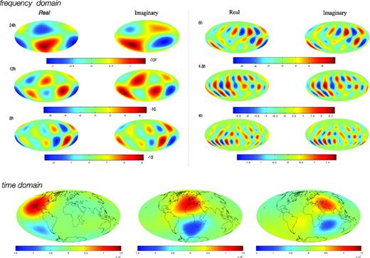
Top: real and imaginary parts of the Sq source in the frequency domain for time harmonic p = 1, 2, …, 6 (24 hr, 12 hr, …, 4 hr) in a stream function (see eq. 30) with the map being centred at 12 LT; bottom: three snapshots of the Sq source in the time domain (16 UT, 12 UT and 8 UT from left to right) showing the current system traveling eastwards. Units are in kA.

Table 2.

External SH coefficients obtained from an Sq equinoctial day of the IQSY data set (19.03.1965) with the potential method; n and m represent SH degree and order and p designates the time harmonic as outlined in eq. (27). These SH coefficients are used for creating synthetic data throughout the paper.

		p = 1 (24 hr)			p = 2 (12 hr)			p = 3 (8 hr)			p = 4 (6 hr)			p = 5 (4.8 hr)			p = 6 (4 hr)
n	m	|$\epsilon _n^m$| [nT]	n	m	|$\epsilon _n^m$| [nT]	n	m	|$\epsilon _n^m$| [nT]	n	m	|$\epsilon _n^m$| [nT]	n	m	|$\epsilon _n^m$| [nT]	n	m	|$\epsilon _n^m$| [nT]
—	—	—	1	1	+0.5504+0.7698i	2	2	−0.3376+0.1315i	3	3	+0.0705−0.1197i	4	4	+0.1053+0.0429i	5	5	+0.0115−0.0486i
1	0	+3.7743−2.4874i	2	1	−0.7030−0.2243i	3	2	+0.1369+0.3717i	4	3	+0.1674−0.1174i	5	4	−0.0720+0.0252i	6	5	+0.0358+0.0666i
2	0	−0.4075+0.7654i	3	1	+0.1313−0.4238i	4	2	−0.3684+0.2006i	5	3	+0.1255−0.1466i	6	4	−0.0421−0.0157i	7	5	−0.0703+0.0133i
3	0	+0.3243−0.1718i	4	1	−0.3225−0.1254i	5	2	+0.6127+0.1570i	6	3	−0.3925−0.0349i	7	4	+0.1021+0.0879i	8	5	+0.0265+0.0494i
1	1	+0.9074+1.3634i	2	2	−0.0242−0.3181i	3	3	+0.2743+0.1639i	4	4	−0.1483−0.2716i	5	5	+0.1076+0.1307i	6	6	−0.0313−0.0487i
2	1	+5.9531+1.6031i	3	2	−3.3878−1.5292i	4	3	+1.3130+1.3031i	5	4	−0.2239−0.4967i	6	5	−0.1355−0.0656i	7	6	+0.0246+0.1115i
3	1	+0.6813+0.0168i	4	2	−0.3569−0.2144i	5	3	−0.0117+0.1397i	6	4	+0.0588−0.0111i	7	5	−0.0093+0.0955i	8	6	−0.0015−0.0318i
4	1	−2.2560+0.3236i	5	2	+0.4190+0.3393i	6	3	+0.1420+0.0183i	7	4	−0.0826−0.1320i	8	5	−0.0862−0.0435i	9	6	+0.0533+0.0485i
2	2	−1.1129+0.9761i	3	3	+0.8457−0.2033i	4	4	−0.3323+0.0945i	5	5	+0.1208−0.0540i	6	6	−0.0792+0.0017i	7	7	−0.0090−0.0086i
3	2	−0.0853+0.2658i	4	3	+0.2489−0.0944i	5	4	−0.0150−0.2011i	6	5	−0.0206+0.1118i	7	6	+0.1328−0.0377i	8	7	−0.0520+0.0157i
4	2	+0.0223−0.5677i	5	3	+0.0171+0.5005i	6	4	−0.1171−0.2231i	7	5	−0.0509+0.0425i	8	6	−0.0119+0.0457i	9	7	+0.0277−0.0185i
5	2	+0.4878+0.5029i	6	3	−0.1804−0.4158i	7	4	+0.0300+0.3342i	8	5	+0.0213−0.0774i	9	6	−0.0016+0.0033i	10	7	+0.0270+0.0108i

With the obtained external coefficients we calculate three magnetic field components at mid-latitude observatories from a 3-D conductivity model of the Earth that includes non-uniform oceans. More exactly, our 3-D model consists of a thin spherical surface layer of laterally variable conductance S(θ, ϕ) and a radially symmetric (1-D) spherical conductivity underneath (Fig. 2). The shell conductance S is obtained by considering contributions both from seawater and sediments. The conductance of seawater has been taken from Manoj et al. (2006) and accounts for the ocean bathymetry, ocean salinity, temperature and pressure. Conductance of the sediments (in continental as well as oceanic regions) is based on the global sediment thicknesses given by Laske & Masters (1997) and calculated by a heuristic procedure similar to that described in Everett et al. (2003). The resolution of the model is chosen to be 1° × 1°. The underlying 1-D conductivity model consists of a 3000 Ohm-m lithosphere with a thickness of 90 km and a layered model underneath, derived from 5 yr of CHAMP, Ørsted and SAC-C magnetic data by Kuvshinov & Olsen (2006). Using these realistic data as input we performed model studies in order to answer the question whether the S3D method indeed outperforms the potential method. We add 0, 5, 10 and 15 per cent Gaussian noise to the data and recovered the external coefficients using the potential and the S3D methods. Table 3 gives the summary of the results. It contains the relative difference (RD) of the ‘true’ and ‘recovered’ external SH coefficients for each time harmonic p from

\begin{equation} RD_{\epsilon }(p)=\frac{ \sqrt{\sum \limits _{n,m}|\epsilon _n^{m,{\rm true}}(\omega _p)-\epsilon _n^{m,{\rm recov.}}(\omega _p)|^2}}{\sqrt{\sum \limits _{n,m}|\epsilon _n^{m, {\rm true}}(\omega _p)|^2}} \times 100, \end{equation}

(31)

which we consider as an intuitive measure of performance of the methods. For the potential method we use all three components (P_XYZ), while for the S3D method we test two versions: when all components are analysed (S3D_XYZ), and when only horizontal components are interpreted (S3D_XY). The subscript designates the components of the geomagnetic field in the XYZ convention, where X = −B_θ is directed to the geographic North, Y = B_ϕ is directed to the geographic East and Z = −B_r is directed downwards. We find that the S3D_XYZ method performs best followed by S3D_XY in recovering the ‘true’ external coefficients throughout all time harmonics. These results are expected since we use exactly the same underlying 1-D section for our synthetic data and our S3D method. The only exception is for RD_ϵ(1) with 15 per cent noise, where P_XYZ gives better results then S3D_XY. The reason for this is not clear but one interpretation is that the noise has most effect on the vertical Z component. By not considering the Z component with the S3D_XY method, some information for accurate source determination is missing.

Table 3.

Table shows the results from our model study of Section 2.3. Noise was added to the realistic but synthetic observatory data and the Sq source was recovered using S3D and the potential method. Numbers in the table are the relative difference RD_ϵ(p), as computed from eq. (31), between ‘true’ and ‘recovered’ coefficients from the S3D_XYZ, S3D_XY and the potential method P_XYZ for time harmonic p. Two successive columns correspond to the results for a specific time harmonic: left-hand column refers to a noise-free 1-D background section, right-hand column refers to a 1-D background section with 15 per cent Gaussian noise. Numbers in brackets in the first line refer to |$\sqrt{\sum_{n,m}|\epsilon _n^{m,{\rm true}}(\omega _p)|^2}$|⁠. Note that the potential method is not influenced by the choice of the conductivity model.

Noise	Method	RDϵ(1)	(8.41)	RDϵ(2)	(4.17)	RDϵ(3)	(2.18)	RDϵ(4)	(0.85)	RDϵ(5)	(0.37)	RDϵ(6)	(0.21)
0 per cent	S3DXYZ	0.0	0.3	0.0	0.4	0.0	0.5	0.0	0.4	0.0	0.5	0.1	0.6
	S3DXY	0.0	0.3	0.0	0.5	0.0	0.6	0.0	0.6	0.0	0.7	0.1	0.8
	PXYZ	4.6	—	5.8	—	7.8	—	7.1	—	6.4	—	7.2	—
5 per cent	S3DXYZ	2.6	2.7	1.2	1.3	0.9	0.9	1.0	1.1	0.9	0.7	0.7	0.7
	S3DXY	2.9	3.1	1.3	1.3	1.0	1.0	1.1	1.3	0.9	0.6	0.7	1.2
	PXYZ	6.1	—	6.1	—	7.4	—	7.1	—	6.2	—	7.5	—
10 per cent	S3DXYZ	7.7	7.8	3.6	3.7	2.8	2.8	3.0	3.1	2.7	2.6	2.1	2.1
	S3DXY	8.8	8.9	3.9	3.9	3.0	2.8	3.2	3.3	2.8	2.3	2.2	2.5
	PXYZ	9.8	—	7.0	—	7.0	—	7.3	—	6.1	—	8.2	—
15 per cent	S3DXYZ	15.3	15.4	7.2	7.3	5.7	5.7	6.1	6.1	5.5	5.3	4.2	4.2
	S3DXY	17.5	17.6	7.9	7.8	6.1	5.9	6.4	6.4	5.6	5.1	4.5	4.6
	PXYZ	16.4	—	9.2	—	7.3	—	8.5	—	7.2	—	9.7	—

Table 4.

Shown is the theoretical penetration depth in kilometres based on the real part of the C-response for Sq (4–24 hr) and D_st (2–107 d) periods and its dependence on SH degree n for the 1-D conductivity model shown in Fig. 2. To estimate the influence of a conducting ocean on top of the 1-D profile, we calculated the penetration depth for three scenarios. ‘No ocean’: 1-D conductivity model, assuming no ocean layer on top. ‘Mean ocean’: a layer with mean of the surface conductance map (8000 S) was added as a top layer to 1-D model. This setup mimics the overall mean influence of a realistic ocean layer. ‘Maximum ocean’: a layer with the maximum of the surface conductance map (20 000 S) was added as top layer to estimate the maximum influence of an ocean surface layer. We find that with decreasing periods, the theoretical penetration depth gets smaller with increasing influence of the ocean. D_st periods of 16–107 d are not largely influenced but the influence is getting stronger within Sq periods.

	Ocean:	No	Mean	Max	No	Mean	Max	No	Mean	Max	No	Mean	Max	No	Mean	Max
Source	Period	n = 1			n = 3			n = 5			n = 7			n = 9
Dst	107 d	1296	1286	1272	1187	1182	1174
	64 d	1121	1111	1095	1053	1046	1035	—	—	—	—	—	—	—	—	—
	32 d	990	977	955	932	922	906	—	—	—	—	—	—	—	—	—
	16 d	894	874	840	846	831	804	—	—	—	—	—	—	—	—	—
	8 d	817	785	727	778	753	704	—	—	—	—	—	—	—	—	—
	4 d	752	696	588	721	673	578	—	—	—	—	—	—	—	—	—
	2 d	688	579	399	665	568	401	—	—	—	—	—	—	—	—	—
Sq	24 hr	612	413	202	596	413	207	570	411	215	534	405	223	494	394	231
	12 hr	514	232	80	507	236	82	493	242	86	473	248	91	447	253	98
	8 hr	449	149	44	446	152	45	438	157	47	426	163	50	410	170	53
	6 hr	403	105	29	401	108	29	397	111	31	390	116	32	379	122	34
	4.8 hr	367	80	21	366	81	21	364	84	22	360	87	23	353	92	24
	4 hr	340	63	16	339	64	16	338	66	17	336	69	18	331	72	18

Table 5.

List of recently installed permanent and non-permanent observatories that were used in the inversion of synthetic data from a realistic observatory distribution.

Observatory name	Location	Longitude	Co-latitude
CKI	Cocos Islands	95.8	102.2
GAN	Maldives	73.1	89.3
NWP	North West Pacific	160.0	48.9
WPB	West Pacific Basin	135.1	70.7
IPM	Easter Island	250.6	117.2
TDC	Tristan da Cunha	347.7	127.1
STH	St Helen	354.3	105.9
SMA	Azores	334.9	53.0
MJR	Majuro	171.2	82.9
PON	Pohnpei	158.3	83.0
MNT	Muntilupa	121.0	75.6
TNG	Tonga	185.0	11.1
MRQ	Marcus Island	153.6	65.82
EM1	North America	239.6	35.9
EM2	—	236.7	44.7
EM3	—	267.0	46.0
EM4	—	253.1	34.0
EM5	—	279.4	37.2
EM6	—	253.7	46.7
EM7	—	264.1	48.4

To make the scenario more realistic we added 15 per cent Gaussian noise to the 1-D conductivity profile when the S3D method is applied. In that way we mimic that we know the 1-D conductivity profile only approximately when using real data. These results appear in the table as a second (right) column for the corresponding time harmonic. Again we find that the S3D_XYZ method gives the best results followed by S3D_XY. We summarize from these studies that the S3D method is a practical concept to recover the Sq source, gives better results than the conventional potential method within our test environment and has advantages as outlined at the end of Section 2.2.

3 RECOVERY OF 3-D MANTLE CONDUCTIVITY WHEN THE SOURCE IS KNOWN

3.1 Formulation

The inverse problem of conductivity recovery is formulated as minimization of the penalty function

\begin{equation} \phi (\mathbf {m,\lambda })=\phi _d(\mathbf {m})+\lambda \phi _S(\mathbf {m}), \end{equation}

(32)

with respect to the model parameter m. Here λ is the regularization parameter, ϕ_S(m) is the regularization term, ϕ_d(m) is the data misfit and m is the vector of model parameters. For our problem the data misfit ϕ_d(m) is written as

\begin{eqnarray} \phi _d (\mathbf {m})&=&\sum \limits _{q=1}^{N_d} \sum \limits _{s \in {\rm Sites} (q)} \sum \limits _{p=1}^{6}\,\Big\lbrace D_{r,s }^q (\omega _p) \left| B_{r,s}^{{\rm mod},q}(\omega _p) - B_{r,s}^{{\rm exp},q}(\omega _p) \right|^2 \nonumber \\ &&+\,D_{\theta ,s }^q (\omega _p) \left| B_{\theta ,s}^{{\rm mod},q}(\omega _p) - B_{\theta ,s}^{{\rm exp},q}(\omega _p)\right|^2 \nonumber \\ &&+\,D_{\phi ,s }^q (\omega _p) \left| B_{\phi ,s}^{{\rm mod},q}(\omega _p) - B_{\phi ,s}^{{\rm exp},q}(\omega _p) \right|^2 \Big\rbrace , \end{eqnarray}

(33)

where |$\mathbf {D}_s^q(\omega _p)$| is a weighting parameter and |$\mathbf {B}_s^{{\rm mod},q}(\omega _p)$| and |$\mathbf {B}_s^{{\rm exp},q}(\omega _p)$| are modelled and experimental magnetic fields, respectively, at location s. The outer sum stresses the fact that we may include data from more than one single day into the inversion (here N_d specifies a number of days, and Sites(q) defines a set of locations for a given q-th day). This idea is motivated by the fact that in this scenario—along with the data from geomagnetic observatories—the data from regional (either surface or/and sea-bottom) EM surveys can be utilized. It is worthwhile to mention here that the sea-bottom observations are especially important since they allow for, at least partially, filling a gap in ground-based data in the oceanic regions. Note that each chosen day is specified by its own source structure, which is known varies with season and solar activity. The reader is referred, for example, to the work of Kuvshinov & Utada (2010) who investigated in detail—on an example of Japanese observatories—the dependence of observed and predicted Sq fields on season and solar activity, as well as on day-to-day variability of the source. In that paper the authors however did not estimate the Sq source themselves but used the Sq source models provided by CM4 (cf. Sabaka et al.2004).

To conclude this section we note that in our inverse setup the regularization term ϕ_S(m) has a form

\begin{equation} \phi _S(\mathbf {m})=(W\mathbf {m})^T(W\mathbf {m}), \end{equation}

(34)

where T means transpose and matrix W approximates 3-D spatial gradient.

3.2 Model parametrization

We define V^inv as the inverse problem domain where we want to recover the 3-D conductivity distribution σ(r). V^inv consists of |$N_r^{\rm inv}$| laterally non-uniform spherical layers, embedded in the Earth's conductivity model, which consists of a surface shell of known laterally varying conductance S(θ, ϕ) and a 1-D background section of known conductivity σ_b(r), as shown in Fig. 4. V^mod designates the forward problem domain where we solve Maxwells's equations. Since the surface shell S(θ, ϕ) largely affects the fields at coastal and island observatories it is important to include it in V^mod, thus V^mod consists of V^inv and a surface shell of conductance S(θ, ϕ). V^mod is discretized into |$N^{\rm mod } = N_r^{\rm mod} \times N_{\theta }^{\rm mod } \times N_{\phi }^{\rm mod }$| volume cells V_i(i = 1, 2, …, N^mod), where |$N_r^{\rm mod }=N_r^{\rm inv }+1$|⁠. The inverse problem domain V^inv is discretized into |$N^{\rm inv } = N_r^{\rm inv } \times N_{\tau }^{\rm inv }$| volume cells V_l(l = 1, 2, …, N^inv), where N_τ designates the number of cells in the horizontal direction. The vector

\begin{equation} \mathbf {m}=(ln(\sigma _1), ln (\sigma _2),\,\ldots,ln(\sigma _{N^{\rm inv }}))^T, \end{equation}

(35)

defines the set of model parameters, where σ_l stands for the conductivity value in the volume cell V_l and superscript T stands for the transpose. The reasoning for the choice of ln(σ_l) is a better scaling of the problem and guarantee of the positiveness of the conductivities during inversion. In the present version of the inverse solution we are free to merge M² cells V_j simultaneously along latitude and longitude within each layer |$N_r^{\rm inv }$|⁠. Thus, for this merging scheme we have

\begin{equation} N_{\tau }^{\rm inv }=\frac{N_{\theta }^{\rm mod }}{M} \times \frac{N_{\phi }^{\rm mod }}{M}, \end{equation}

(36)

with merging parameter M.

Figure 4.

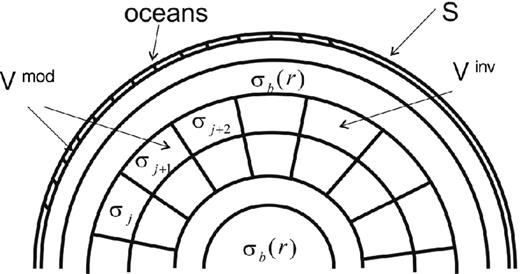
Parametrization of 3-D model domain.

3.3 Limited-memory quasi-Newton method

We apply the limited-memory quasi-Newton method to minimize our penalty function in eq. (32). We follow the algorithm from Nocedal & Wright (2006), which uses an iterative update of the trial solution

\begin{equation} \mathbf {m}_{k+1}=\mathbf {m}_k+\alpha _k\mathbf {p}_k, \end{equation}

(37)

where p_k is determined as

\begin{equation} \mathbf {p}_k=-B_k^{-1}\nabla \phi _k. \end{equation}

(38)

Here k designates the number of iteration, α_k is the step length, |$B_k^{-1}$| is the Broyden-Fletcher-Goldfarb-Shanno (BFGS) approximation of the inverse Hessian and

\begin{equation} \nabla \phi _k=\left( \frac{\partial \phi }{\partial m_1},\frac{\partial \phi }{\partial m_2},\,\ldots,\frac{\partial \phi }{\partial m_{N^{\rm inv }}}\right)^T \bigg |_{\mathbf {m}=\mathbf {m}_k}, \end{equation}

(39)

is the gradient vector with respect to the model parameters m_k. To compute ∇ϕ_k we have to calculate the data misfit |$\nabla \phi _d\big |_{\mathbf {m}=\mathbf {m}_k}$| and the regularization term |$\nabla \phi _S\big |_{\mathbf {m}=\mathbf {m}_k}$|⁠. Following the formalism of Pankratov & Kuvshinov (2010) one can obtain the derivative of the data misfit with respect to model parameters as

\begin{eqnarray} \!\!\!&&&&{\frac{\partial \phi _d}{\partial m_l}=2\sigma _l \Re \Bigg\lbrace \sum \limits _{q=1}^{N_d}\sum \limits _{p=1}^{6}\int _{V_l} \big[E_r^q(\mathbf {r},\omega _p)E_r^{A,q}(\mathbf {r},\omega _p)} \nonumber \\ \!\!\!&&\quad+\, E_{\theta }^q(\mathbf {r},\omega _p)E_{\theta }^{A,q}(\mathbf {r},\omega _p) + E_{\phi }^q(\mathbf {r},\omega _p)E_{\phi }^{A,q}(\mathbf {r},\omega _p)\big] \ {\rm d}v \Bigg\rbrace , \end{eqnarray}

(40)

where V_l ∈ V^inv(l = 1, 2, …, N^inv) and ℜ stands for the real part. Here E^q is the ‘electric field’ solution of Maxwell's equations

\begin{equation} \frac{1}{\mu _0}\nabla \times \mathbf {B}^q=\sigma \mathbf {E}^q+\mathbf {j}^{\rm ext,q}, \end{equation}

(41)

\begin{equation} \nabla \times \mathbf {E}^{q}={\rm i}\omega _p\mathbf {B}^{q}, \end{equation}

(42)

where j^{ext, q} is the Sq source for q-th day (note that B^q corresponds to B^{mod, q} in eq. 33). ‘Adjoint’ field, E^{A, q}, is the electric field solution of Maxwell's equations

\begin{equation} \frac{1}{\mu _0}\nabla \times \mathbf {B}^{A,q}=\sigma \mathbf {E}^{A,q}, \end{equation}

(43)

\begin{equation} \nabla \times \mathbf {E}^{A,q}={\rm i}\omega _p \mathbf {B}^{A,q}+\mathbf {h}^q, \end{equation}

(44)

where an adjoint ‘magnetic’ source, h^q is given by

\begin{equation} \mathbf {h}^q(\mathbf {r},\omega _p)= \sum \limits _{s \in {\rm Sites}(q)} \mathbf {M}^q(\mathbf {r}_s,\omega _p)\delta (\mathbf {r}-\mathbf {r}_s), \end{equation}

(45)

with

\begin{eqnarray} \mathbf {M}^q(\mathbf {r},\omega )& = & D_{r }^q (\mathbf {r},\omega ) \left( B_{r}^{{\rm mod},q}(\mathbf {r},\omega ) - B_{r}^{{\rm exp},q}(\mathbf {r},\omega ) \right)^* \mathbf {e}_r\nonumber \\ &&+\,D_{\theta }^q (\mathbf {r},\omega ) \left( B_{\theta }^{{\rm mod},q}(\mathbf {r},\omega )- B_{\theta }^{{\rm exp},q}(\mathbf {r},\omega )\right)^* \mathbf {e}_{\theta }\nonumber \\ &&+\,D_{\phi }^q (\mathbf {r},\omega ) \left( B_{\phi }^{{\rm mod},q}(\mathbf {r},\omega )- B_{\phi }^{{\rm exp},q}(\mathbf {r},\omega ) \right)^* \mathbf {e}_{\phi }. \end{eqnarray}

(46)

Here * denotes the complex conjugate. Note that the gradient of the regularization term ∇ϕ_S can be computed analytically, using eq. (34), as

\begin{equation} \nabla \phi _S=2W^TW\mathbf {m}. \end{equation}

(47)

The final remark of this section concerns the numerical solution of eqs (41) and (42) and eqs (43) and (44), which are needed to predict the magnetic field B^q and the electric fields, E^q and E^{A, q} within the volume cells V_l. We solve these equations using a 3-D spherical EM induction code (Kuvshinov et al.2002; Kuvshinov 2008), which is based on the contracting IE approach (cf. Pankratov et al.1995; Singer 1995). For details of the inversion scheme the interested reader is referred to Kuvshinov & Semenov (2012), where the scheme is fully explained, including the efficient implementation and the explicit derivation of Green's tensor functions, which are needed for the numerical realization of the IE approach.

3.4 Numerical verification of the 3-D inverse solution when the source is known

The test in this section can be considered as a proof of concept, aiming to answer the question whether our implementation of optimization method, along with the adjoint approach as applied to our data, works correctly. The setup for the synthetic data and the inversion setup are as follows.

3.4.1 Synthetic data setup

We use a realistic Sq source (Table 2) to calculate magnetic fields for 1 d (N_d = 1) at a regular 5° × 5° grid of observation sites by solving Maxwell's equation for the following 3-D model. We use an outer 2-D non-uniform land/ocean surface conductance shell followed by an inhomogeneous anomaly layer at 300 km depth with 100 km thickness embedded in the 1-D background conductivity section as shown in Fig. 2. The conductivity of the ‘true’ anomaly model has a 60° checkerboard structure along longitude and co-latitude and varies by |$\sigma _b / \sqrt{10}$| and |$\sigma _b \sqrt{10}$| from the 1-D background section σ_b at the respective depth. The forward model discretization is 5° × 5° resulting in 2592 cells per layer.

3.4.2 Inversion setup

We assume to be exactly known: (1) the background 1-D conductivity; (2) the source; and (3) the location (depth and thickness) of the inhomogeneous layer. During inversion the conductance of the surface shell was fixed. No data weighting is introduced [|$\mathbf {D}_s^q(\omega _p)=1$|], no merging (M = 1) is implemented, no noise is added and no regularization is used (λ = 0). The inverse model discretization is also 5° × 5°. The inversion starts from the 1-D background conductivity value σ_b in this depth.

Fig. 5 shows the results of this test inversion. After 257 iterations the misfit drops from the initial value of 180 by about three orders of magnitude to 0.25.

Figure 5.

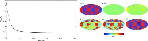
Results of the numerical verification of 3-D conductivity recovery when the source is known (see details in Section 3.4). Left-hand side: misfit with respect to iterations; after 257 iterations the misfit drops from the initial value of 180 by about three orders of magnitude to 0.25. Right-hand side: ‘true’ model which is to be recovered, the inversion starting model, the inversion results after 1, 5, 10 iterations and the final result after 257 iterations. Conductivities are given in log₁₀(σ).

We summarize from this test that with the complex Sq source described from 71 external SH coefficients for all six time harmonics, the inverse scheme gives an almost perfectly recovered conductivity distribution within our test environment.

4 RESOLUTION STUDIES

In this section we discuss the spatial resolution of our method for two synthetic data sets, one—from a regular grid of observations, and another—from a realistic observatory distribution. We investigate the influence on the results of different inverse setups. In particular, we discuss the results when all components (XYZ) and only the vertical component (Z) are inverted. Also, we examine how different period ranges (Sq or Sq plus D_st) affect the resulting images. The logic of our resolution study closely follows that of Kelbert et al. (2008). However, we want to emphasize that the setups are very different, especially for Sq periods, where we work with a realistic Sq source while Kelbert et al. (2008) exploit a simplified |$P^0_1$| source for this period range. In addition, we work—as described in previous sections—with the time spectra of the fields in contrast to Kelbert et al. (2008) who work with response functions.

4.1 Resolution studies with a regular grid of observations

In this section we investigate the resolution of the inverse solution in vertical and lateral directions if a hypothetical dense and regular grid of observations is provided. The setup for these model studies is as follows.

4.1.1 Synthetic data setup

We again use a realistic Sq source in the period range of 4–24 hr (Table 2), and optionally a D_st source described by |$Y^0_1$| harmonic in the period range of 2–107 d, to calculate magnetic fields on a regular 5° × 5° grid of observatory sites. We use a 2-D non-uniform land/ocean surface conductance shell followed by eight layers (either laterally homogeneous or inhomogeneous) between 10 and 1600 km depth, embedded in the 1-D background section. The depth ranges of these eight layers are 10–100 km, 100–250 km, 250–410 km, 410–520 km, 520–670 km, 670–900 km, 900–1200 km and 1200–1600 km, respectively. Eight data sets are prepared. The first data set is for the 3-D model where the target layer with a laterally inhomogeneous conductivity distribution is located in depth from 10–100 km, with other layers being laterally homogeneous and having the conductivity of 1-D background section. The second data set is for the 3-D model where the target layer with inhomogeneous conductivity is located in depth range from 100 to 250 km, with other layers being laterally homogeneous, and so forth. The conductivity within the inhomogeneous layer has a 60° checkerboard structure along longitude and co-latitude and varies by |$\sigma _b / \sqrt{10}$| and |$\sigma _b \sqrt{10}$| from the 1-D background section σ_b at the respective depth (see Fig. 6 for the reference checkerboard to compare with the inversion results). The forward model discretization is 5° × 5° resulting in 2592 cells per layer. With these eight data sets we perform a resolution study, which exemplifies in Fig. 7 (the results presented in this figure are discussed in more detail later in this section). The n-th column (from the left to the right) corresponds to 3-D inversion of n-th data set, where during 3-D inversion we assume that all eight layers are inhomogeneous and thus we search conductivity distributions in all these layers. Note that with perfect data the 8 × 8 matrix of maps in Fig. 7 should have diagonal form with the true checkerboard conductivity distributions at the diagonal.

Figure 6.

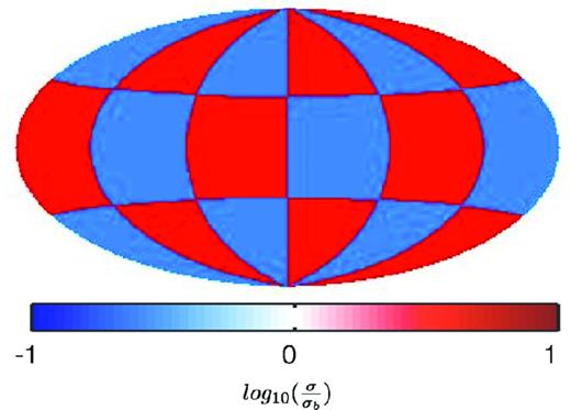
Reference checkerboard of 60° anomaly structure along longitude and co-latitude with conductivities of |$\sigma _b / \sqrt{10}$| and |$\sigma _b \sqrt{10}$|⁠, where σ_b is the conductivity of the respective depth in the 1-D background section. The model is centred on the zero meridian.

Figure 7.

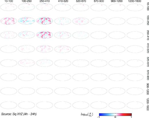
Results of the resolution study from Sq XYZ data. Every column represents an individual inversion with the target checkerboard anomaly of |$\sigma _b /\sqrt{10}$| and |$\sigma _b \sqrt{10}$| changing its depth increasingly from 10–100 km (first column) to 1200–1600 km (eighth column). Horizontal aligned numbers on top designate the depth of the checkerboard anomaly for the respective column, vertical aligned numbers on the right designate the vertical inverse domain discretization. Conductivities are given in log₁₀(σ/σ_b). View is centred on the zero meridian. The surface conductance map from 0 to 10 km depth is used for the modelling but not shown here.

4.1.2 Inversion setup and results

We use the same inversion setup as outlined in Section 3.4 but now with eight homogenous layers.

With this setup we first perform a resolution study where all Sq magnetic components (XYZ) are used during inversion. Fig. 7 demonstrates that the recovered target at the respective depth is poorly resolved. The maximum sensitivity is observed between 100 and 410 km. If the target is located deeper it is not resolved at all. To investigate whether the resolution is influenced by the surface conductance, we calculated the theoretical penetration depth (which governs the vertical resolution), based on the real part of the C-response, in a spherical conductor for Sq (4–24 hr) and D_st (2–107 d) periods and its dependence on the SH degree n for the 1-D conductivity model shown in Fig. 2. To estimate the influence of a conducting ocean on top of the 1-D profile, we calculated the penetration depth for three scenarios. For case 1 (‘No ocean’) we used the original 1-D model, assuming no ocean layer on top. For case 2 (‘Mean ocean’) we use the mean conductance of the ocean (8000 S). This setup mimics the overall mean influence of the ocean layer. For case 3 (‘Maximum ocean’) we use the maximum conductance of the ocean (20 000 S) to estimate the maximum influence of an ocean layer. One can see from Table 4 that with decreasing periods, the theoretical penetration depth gets smaller with increasing influence of the ocean. While D_st periods of 16–107 d are not significantly influenced, the effect is getting stronger at shorter periods (especially at Sq periods), decreasing the theoretical penetration depth down to 200 km even at the maximum Sq period of 24 hr.

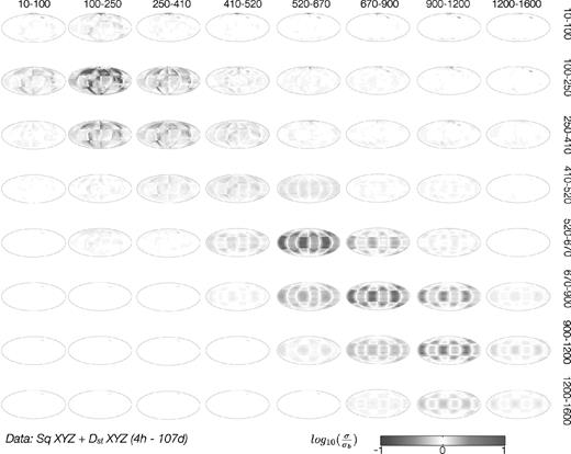
These results lead us to a further test where we use XYZ data from a synthetic D_st source in addition to Sq XYZ data to check if the inversion results could be improved. D_st data were computed at periods of 2, 4, 8, 16, 32, 64 and 107 d. Fig. 8 demonstrates the results of the inversion of this data set. It is clearly seen from the figure that by including D_st data one can indeed improve (as expected) the resolution down to 1600 km. By comparing the results visually we find that structure with good conductivity is better resolved than the parts of the checkerboard anomaly with low conductivity. However we still find artefacts in the layers above and under the actual target layer.

Figure 8.

Results of the resolution study from Sq XYZ and D_stXYZ data. The same legend as in Fig. 7.

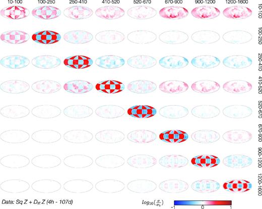
As a further test we again invert both Sq and D_st data, but now only Z component. As seen in Fig. 9, the recovery of the target conductivity is tremendously improved in both vertical and horizontal directions in all layers. This encouraging result is not completely surprising; it is well known that the vertical magnetic component is more sensitive to 3-D variations of conductivity than the horizontal components. From visual comparison we observe the best recovery in the depth range of 100–250 km.

Figure 9.

Results of the resolution study from Sq Z and D_stZ data. The same legend as in Fig. 7.

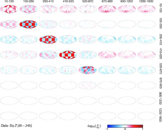
Then we invert only Sq Z data. From the results presented in Fig. 10 we conclude that by inverting Sq Z data one can resolve the structures down to 670 km. Again, we observe that the best resolution is achieved in the depth range of 100–250 km.

Figure 10.

Results of the resolution study from Sq Z data. The same legend as in Fig. 7.

As an ultimate run we investigate how the results would change if noise is added to the data. This also verifies our regularization scheme. We again invert only Sq Z data but now with 3 per cent Gaussian noise. To determine a proper regularization parameter λ in eq. (32) we use the L-curve approach (Hansen 1992). From theory the optimal regularization parameter λ lies in the knee of the L-curve. For all runs we obtained L-curve shapes comparable to that shown in Fig. 13 and we picked up the solution for optimal λ. Fig. 11 shows the results for this set of tests. Now we succeeded to resolve the structures down to 520 km, and, as in previous test, the best resolution is obtained in the depth range of 100–250 km.

Figure 11.

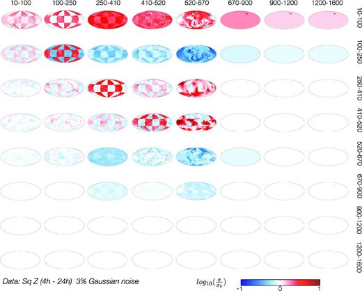
Results of the resolution study from Sq Z data with 3 per cent Gaussian noise and applied regularization. The same legend as in Fig. 7.

We summarize from these resolution studies that: (1) inverting Z component gives much better results than inverting all components; (2) data from the Sq source allows for resolving 3-D structures in depth range between 100 and 520; (3) the best resolution is achieved in the depth range of 100–250 km and (4) as expected, adding data from a D_st source one resolves the structures down to 1600 km.

4.2 Resolutions studies with a realistic distribution of observatories

The previous section discusses the inversion results obtained when the data from a regular and dense net of observations were used. In this section we present the results where synthetic data from a global net of geomagnetic observatories were employed.

4.2.1 Synthetic data setup

We use the similar 3-D multilayered setup as in Section 4.1 and the same Sq source. This time we focus on the depth range in between 100 and 520 km where we found (see previous section) Sq data have the highest sensitivity. Note that we omit high-latitude (>60°) and low-latitude observatories (<6°) to minimize the influence of the auroral and equatorial electrojets as would be the case when working with real data. We computed data on the real observatory positions from the IQSY as presented in Table 1 and added 3 per cent Gaussian noise. In addition we computed the data at a number of non-permanent and permanent geomagnetic observatories, which have been recently installed and which improve the coverage, especially in oceanic areas and the southern hemisphere (their location is shown by red stars in Fig. 12). Table 5 summarizes the information about these sites. Since 2007 the ‘German Research Centre for Geosciences’ (GFZ, Potsdam) operates a geomagnetic observatory on St Helena Island in the South Atlantic (Korte et al.2009) and since 2010 on Santa Maria on the Azores. Also in the South Atlantic, the Danish ‘National Space Institute’ (‘DTU Space’, Lyngby) runs an observatory on Tristan da Cunha Island (Matzka et al.2009). Furthermore, an observatory has been installed in the South Pacific Ocean on the Easter Islands in 2008, operated from the French ‘Institut de Physique du Globe de Paris’ (‘IPGP’, Paris) in cooperation with the Chilean Meteorological Service (‘Direccion Meteorologica de Chile’, Santiago; Chulliat et al.2009). Since 2012 the‘Swiss Federal Institute of Technology’ (‘ETH’, Zürich) runs a geomagnetic observatory on Gan Island (Maldives) in cooperation with the ‘Maldivian Meteorological Service’ (Male) and the Indian ‘National Geophysical Research Institute’ (NGRI, Hyderabad), and an observatory on Cocos Islands, in cooperation with ‘Geoscience Australia’ (Canberra; Velimsky et al.2012). Also ‘Ocean Hemisphere Research Center’ (OHRC) from the Japanese ‘Earthquake Research Institute’ (ERI, Tokyo; Shimizu & Utada 1999) installed five long-term geomagnetic stations—Majuro (Marshall Islands), Pohnpei (Micronesia), Muntinlupa (Philippines), Atele (Tonga), Marcus Island (Japan)—in the Pacific Ocean within the ‘Ocean Hemisphere Network Project’ (1996–2000). As a further option we included the seven backbone long-period MT stations in North America from the NSF ‘Earthscope’ project (Schultz 2010). Finally, in order to demonstrate the usage of sea-bottom observatories, we included the two observatories ‘NWP’ (North West Pacific) and ‘WPB’ (West Philippine Basin) from Toh et al. (2004, 2006, 2010) who reported their successful long-term operation.

Figure 12.

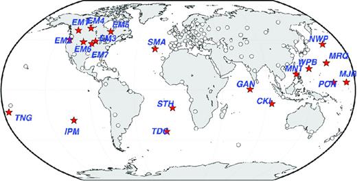
Magnetic observatory network with observatories from the ‘IQSY’ (white dots) and recently installed non-permanent and permanent observatories (red stars) which improve the coverage especially in oceanic sites and the Southern Hemisphere. See text for details.

4.2.2 Inversion setup and results

We use the similar setup as in Section 3.4, but in this scenario we concentrate on the depth range from 100 to 520 km. We invert only for Sq Z component, use a merging factor of M = 6, and implement a regularized solution. The results of the inversion are shown in Fig. 14. We determine the regularization parameter λ on the basis of the L-curve criterion (Fig. 13). However, we observed that plotting the misfit against the regularization term of various regularization parameters λ in the range of no regularization (λ = 0) to an over-regularized solution (λ = 10¹²) does not necessarily have a typical L-curve appearance. The presented L-curve in Fig. 13 is for inversion run when the target layer is placed at depths 100–250 km, where we found the resolution to be maximum. Summarizing, we find the results from the previous tests confirmed, in that the higher conducting parts of the checkerboard anomaly in depth of 100–250 km are best resolved. We also find that the vertical resolution in the global setup is not optimal but good results can be achieved in areas of dense observatory coverage. Expanding this concept to the inversion of real data, a semi-global approach (Fukao et al.2004; Koyama et al.2006; Utada et al.2009; Shimizu et al.2010) of areas with relatively dense coverage could be more attractive in a sense of improving the horizontal resolution of the UM structures in a depth range of 100–520 km.

Figure 13.

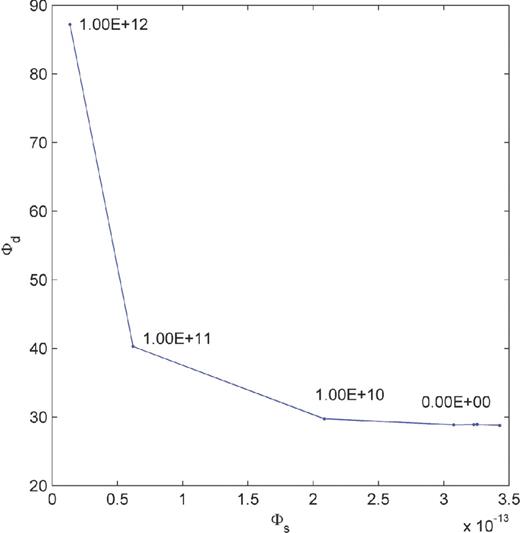
Respective L-curve from the inversion of Sq Z data in Fig. 14 for a target layer in 100–250 km depth.

Figure 14.

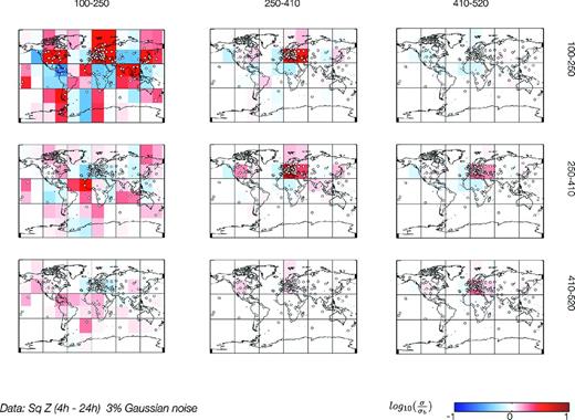
Results of the resolution study with a realistic net of observations from Sq Z data with 3 per cent Gaussian noise and applied regularization. The legend is similar to that in Fig. 7.

5 SIMULTANEOUS SOURCE AND CONDUCTIVITY DETERMINATION

In this section we test the overall scheme for the simultaneous source and conductivity determination as outlined in Fig. 1. To demonstrate its performance we adopt the following data and inversion setups.

5.1 Synthetic data setup

We use the similar setup as outlined in Section 4.1 and calculate Sq magnetic fields for a regular 5° × 5° grid of observatory sites. The ‘true’ anomaly model has again a 60° checkerboard structure at a depth of 100–250 km (Fig. 15) where the best resolution was reported in previous sections. We added 3 per cent Gaussian noise to the data.

Figure 15.

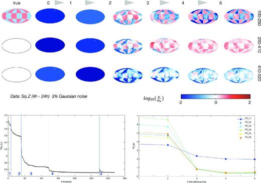
Results of the simultaneous Sq source and conductivity determination (see details in Section 5). Top columns: evolution of conductivity recovery. True model which is to be recovered, staring model (0) and inversion results after five simultaneous loops. Bottom left: Misfit ϕ_d for five external loops. Parts of curves separated by vertical lines correspond to evolution of misfit within ‘internal’ iteration when we recover conductivity distribution with a fixed source. Bottom right: RD_ϵ(p) for p = 1, 2, …, 6 as measure for the misfit of the source. As it is seen the Sq source determination and conductivity recovery is improving with every external iteration.

5.2 Inversion setup and results

We use the similar setup as in Section 4.2 with a merging factor of M = 2. For the initialization of the overall scheme (see upper block of Fig. 1) we use a starting model which strongly deviates from the true model in all three inversion layers (see Fig. 15) and do not fix the source but update it during the inversion as explained in Fig. 1.

To monitor the results we compute RD_ϵ(p) from eq. (31) with p = 1, 2, …, 6 for 5 simultaneous (external) loop iterations as outlined in Fig. 1. The evolution of the misfit ϕ_d and RD_ϵ(p) along with the inversion results are shown in Fig. 15. Since we start with a model which differs from the target model, the Sq source is poorly recovered after the first external iteration. RD_ϵ(p) shows an offset from 4 per cent up to 7 per cent in all time harmonics. As expected, using this Sq source during 3-D inversion does not give a perfect conductivity recovery and the misfit ϕ_d is only slightly reduced. Entering the next external loop and using the updated conductivity model as a starting model leads to better Sq source recovery, which is seen as a slight decrease of RD_ϵ(p) in all time harmonics. This more accurate Sq source leads to a better inversion result at the next external iteration and the high conducting part of the checkerboard appear in the top two layers. This procedure is looped 5 times until the solution converges and we obtain finally a good description of the true Sq source and true 3-D structure. However we note rather strong artifacts in the second and third layers which in theory should be laterally homogeneous. Also the improvement of Sq source for the 24 h period (p = 1) is not as good as for other time harmonics, for which we do not have a solid explanation. However, in overall, especially bearing in mind that we started from the model which is substantially differs from the true model, the results of this section seems to be very encouraging, and we consider them as a proof of concept. Indeed we demonstrate that the looped sequential scheme of simultaneous determination of the source and conductivity allows for recovery of both (source and conductivity) components. The application of the concept to real data within a semi-global paradigm will follow in a future publication.

6 CONCLUSIONS

We present a novel global 3-D EM inverse solution that allows for working in an unified and consistent manner with frequency-domain data originated from both ionospheric and magnetospheric sources irrespective of their spatial complexity. The two key ideas behind this concept are: (1) one has to work with the fields (more exactly with the time spectra of the fields) rather than with the responses; (2) one has to determine simultaneously the parameters describing the source and conductivity distributions in the Earth. Such determination is implemented in our inverse solution as a looped sequential procedure that involves two steps: determination of the source using a fixed 3-D conductivity model and recovery of a 3-D conductivity model using a fixed source. We performed model studies to verify each step separately and together, by using the data synthesized in realistic 3-D Earth's models induced by a realistic Sq source. As far as we know, there were no attempts hitherto to invert Sq data (either synthetic or observed) in the frame of 3-D conductivity models of the Earth.

To determine the source we implement an approach which makes use of the known 3-D conductivity structure of the Earth with non-uniform oceans. Based on model studies we show that this approach is a practical concept to recover the Sq source and it indeed gives better results than the conventional potential method within our test environment. In addition this method allows us to include sea-bottom data into the analysis. This is not possible with the potential method since the sea-bottom observations are performed within a conductor where the potential representation of the magnetic field is no more valid. Finally one can incorporate electric field data into the scheme if such data are available. Again this is not feasible with the potential method even at the surface of the Earth, since the time-varying electric field is nowhere a potential field.

As for recovery of 3-D conductivity our inverse scheme closely follows an inverse scheme described in Kuvshinov & Semenov (2012). It is based on a regularized least-squares formulation, exploits a limited-memory quasi-Newton optimization method and makes use of the adjoint source approach to calculate efficiently the misfit function gradient. Since the new approach presented here works with the time spectra of the magnetic field instead of the C-responses, we modify the misfit gradient calculations by elaborating a new adjoint source. The scheme was successfully verified using the data synthesized in a 3-D model with non-uniform oceans and mantle inhomogeneity induced by a realistic Sq source. With these developments in hand we verified the overall scheme, which iteratively updates both the source and conductivity distribution.

We perform comprehensive resolution studies with checkerboard conductivity structures at depths between 10 and 1600 km for different inverse setups. Our main findings from these studies are: (1) inverting Z component gives much better results than inverting all (X, Y and Z) components; (2) data from the Sq source allow for resolving 3-D structures in depth range between 100 and 520; (3) the best resolution is achieved in the depth range of 100–250 km and (4) as expected, adding data from a D_st source one resolves the structures down to 1600 km.

7 OUTLOOK

In this paper we discuss the concept as applied to synthetic Sq data. The natural next step is implementing the concept to real Sq data in order to resolve conductivity distributions at UM depths.

While not overlooking about the general non-trivial task of working with Sq data, due to the complex spatial structure of the Sq source, we want to stress one important advantage of Sq data compared with D_st data. It is known that analysis of D_st variations requires very long continuous time-series (of a few years or so) and this fact considerably limits the number of observation sites, which might be included in such analysis. Seemingly, only data from a global net of geomagnetic observatories can be used for this aim. With Sq signals—since they are periodic—one can work on a single-day basis, which allows for using data from regional EM surveys along with the data from geomagnetic observatories. In this context, a semi-global approach (Fukao et al.2004; Koyama et al.2006; Utada et al.2009; Shimizu et al.2010), focused on areas of dense coverage from permanent and non-permanent sites, could be an approach of choice on a way to improve the horizontal resolution of the recovered models. A good example of such a survey is the ‘Australia Wide Array of Geomagnetic Stations’ (AWAGS) experiment, within which an array of 57 instruments was distributed regularly across the Australian continent and continuously measured the magnetic field during 1 yr (1991), providing data in the otherwise poorly covered southern hemisphere (cf. Chamalaun & Barton 1993). Another example of a regional survey is the sea-bottom MT experiment in the Philippine Sea (cf. Baba et al.2010), which provides 1 yr of data from 21 sites in the ocean region (it is interesting that for MT analysis Sq variations are usually considered as a source of noise and as a rule are filtered out before further MT analysis). Note that the sea-bottom observations are especially important since they allow for, at least partially, completion of a huge gap in ground-based data in oceanic regions. However with the sea-bottom data one should realize that these data are generally contaminated by motionally induced fields from ocean tides. Tidal signals are also periodic with periods being very close to diurnal and semidiurnal periods of Sq. Therefore the sea-bottom Sq signals must be separated from tidal constituents (noises in this case) as accurate as possible. This is a challenging task, which can be addressed, for example, by detailed 3-D modelling of the tidal signals (in time domain) for a specific day using comprehensive realistic models of tidal velocities (cf. Erofeeva & Egbert 2002), with subsequent subtraction of modelled tidal signals from the observation.

Another issue we intend to address is a better description of the Sq source. In this paper we followed the recipe by Schmucker who introduced a specific subset of SH to describe the Sq source. In future, we plan to make this scheme more flexible, for example, by implementing regression analysis (cf. Kleinbaum et al.1987) to detect statistically significant SH. It is relevant to mention here that we confine ourselves to working with mid-latitude ground-based data only. This influential decision is motivated by our intention to avoid the complications arising if one works with the data from low and high latitudes where the signals from equatorial and polar electrojets dominate. It is known that these sources have spatially small-scale structures and thus the ground-based data coverage is probably not sufficient to describe these sources using either low-order SH or more appropriate spatial forms, for example, quasi-dipole basis functions (Emmert et al.2010). In addition, due to small-scale features of these sources (and the considered period range) the corresponding signals only weakly depend on the Earth's conductivity, as was shown in Kuvshinov et al. (2007) and Semenov & Kuvshinov (2012).

In the presented inversion solution the volume cells, where the conductivities are searched for, are assumed to cover uniformly (in lateral directions) the inverse volume. A more flexible option of the inverse volume parametrization seems to be more appropriate for ground-based data. For example discretization of the inverse volume can be made denser beneath the regions with better data coverage and sparser in the regions with a few data.

Finally we plan to include D_st data to make the analysis as complete as possible.

The authors thank William Lowrie and Amir Khan for help with refining the English presentation of this paper. We are thankful to two anonymous reviewers for their detailed comments and suggestions on how to improve the manuscript. SK thanks Christoph Püthe on discussion of regularization of global EM inversion problems. This work has been supported by SNF grant No. 2000021-121837/1, and in part by the Russian Foundation for Basic Research under grant No. 12-05-00817-a. The authors also express their gratitude to the staff of the geomagnetic observatories who have been collecting and distributing the data.