Enhancing core-diffracted arrivals by supervirtual interferometry

Abstract

A supervirtual interferometry (SVI) method is presented that can enhance the signal-to-noise ratio (SNR) of core diffracted waveforms by as much as |$O(\sqrt{N})$|⁠, where N is the number of inline receivers that record the core–mantle boundary (CMB) diffractions from more than one event. Here, the events are chosen to be approximately inline with the receivers along the same great circle. Results with synthetic and teleseismic data recorded by USArray stations demonstrate that formerly unusable records with low SNR can be transformed to high SNR records with clearly visible CMB diffractions. Another benefit is that SVI allows for the recording of a virtual earthquake at stations not deployed during the time of the earthquake. This means that portable arrays such as USArray can extend the aperture of one recorded earthquake from the West coast to the East coast, even though the teleseism might have only been recorded during the West coast deployment. In summary, SVI applied to teleseismic data can significantly enlarge the catalogue of usable records both in SNR and available aperture for analysing CMB diffractions. A potential drawback of this method is that it generally provides the correct kinematics of CMB diffractions, but does not necessarily preserve correct amplitude information.

Time-series analysis, Interferometry, Core, outer core and inner core, Body waves, Wave scattering and diffraction, Indian Ocean

1 INTRODUCTION

Early seismic inferences about the Earth's deep interior were made by comparing earthquake records against predictions from simple earth models. Trial and error adjustments of the model to fit the data were used to explain the observed seismograms, which led to key discoveries about the Earth's inner and outer cores, mantle and Moho discontinuity. Subsequently, global tomography (e.g. Rawlinson et al.2010) provided the reconstruction of large-scale 3-D velocity variations of the crust, subduction zones, mantle structure and mantle plumes (Walck & Clayton 1984; Woodhouse & Dziewonski 1984; Zelt & Smith 1992; Shearer 2009; Stein & Wysession 2009). More recently, the advent of inexpensive distributed computing promoted the increasing use of full-wave techniques for modelling and inverting earthquake data (e.g. Komatitsch & Tromp 2002; Nissen-Meyer et al.2007; Tape et al.2010) to improve the resolution of 3-D earth models. Thus, at least within a limited frequency band, we are at the stage where computational power allows for the inversion of waveforms in realistic settings.

However, a chief impediment in global seismology and tomography is the limited and irregular distribution of recording stations and earthquakes with acceptable signal-to-noise ratio (SNR). Earthquake recording stations are mainly restricted to land areas of the Earth, and most are sparsely distributed except for certain areas, for example, in the United States, Europe and Japan. Significantly better imaging of the Earth requires a significantly improved number and quality of seismograms and a wider source–receiver coverage. Hence, important improvements in understanding the Earths interior will likely proceed at the pace of increasing the quality of noise-suppressed seismograms available for reliable Earth imaging.

The advent of large-scale portable and permanent seismic arrays (USArray, many European arrays, Japan and China) is quickly changing the way in which global seismic data is being processed, interpreted and used. It is therefore timely to exploit the benefits of having such dense coverage on the station side, including the inline arrangement over vast distances. Waves diffracted around the core–mantle boundary (CMB) assume a central role in covering the lowermost mantle, a region that is key to understanding the dynamics of both the mantle and the core (Lay & Garnero 2004). This bottom thermal boundary layer of mantle convection is subject to interdependent multiscale structures covering heterogeneities on the scale of kilometres (ULVZ) to thousands of kilometres (LLSVPs). First-arriving Pdiff and Sdiff phases are recorded at wide frequency ranges (easily down to a few seconds) and therefore provide a valuable resource for multiscale imaging. They also sample a larger fraction of the CMB region than any other seismic phase by means of their lateral propagation path over great distances. Thus, they are crucial to improving our understanding of this region which is notoriously undersampled due to its remote inaccessibility. Diffracted wave arrivals have been routinely collected (Ritsema, personal communication, Garnero, personal communication), but rarely used in tomography due to issues related to (1) correct modelling and (2) SNRs. Diffracted waves need to be modelled with full-wave theory because they continuously scatter energy away into the mantle, leading to smaller and smaller SNRs with increasing recording distance. It is therefore of interest to increase the SNR, especially for large distances.

We propose to increase the number of usable records by using supervirtual interferometry (SVI; Bharadwaj & Schuster 2010; Mallinson et al.2011; Bharadwaj et al.2012) to transform noisy records into signal. The SVI method was originally developed to increase the SNR of head-wave arrivals by a factor proportional to |$\sqrt{N}$|⁠, where N is the number of sources post-critically offset from the receivers in a conventional survey. It was suggested in Bharadwaj et al. (2012) that this method could be applied to head-wave refractions (Pn and Sn phases) from upper-mantle discontinuities (Shearer 2000; Deuss 2009) and to diffractions (Dai et al.2011; Ruigrok et al.2012) such as those from the CMB boundary. Diffracted waves especially at high frequencies (seismic periods at 5 s and below) scatter energy very intensely such that these arrivals are difficult to detect above the noise level, but are especially interesting for coverage of small-scale structures in the region just above the CMB. As an example, Pdiff waves undergo strong scattering and are therefore difficult to detect at large distances. Sdiff waves scatter less and exhibit better SNR, but are still difficult to detect in raw data at large distances and high frequencies (seismic periods between 1 and 5 s). Both wave types can therefore significantly benefit by increasing their SNR.

We now present the theory of SVI for enhancing the SNR of core-diffracted earthquake waves that propagate along the CMB. This theory is validated using both synthetic data and teleseismic data recorded by USArray. The hypocentres are mainly located near the coast of Indonesia and range from magnitude 5.5 to more than 7.5. There are two significant advantages in generating supervirtual diffraction arrivals by SVI.

• The poor SNR of CMB diffractions associated with weak magnitude teleseisms can be enhanced by interferometrically combining weak and large magnitude events. This can significantly enlarge the number of useful core-diffracted arrivals for analysing the CMB.

• SVI allows for the virtual recording of an earthquake at stations not deployed during the time of the earthquake. This means that transient arrays such as USArray can extend the recording aperture of one recorded earthquake from the West coast to the East coast, even though the teleseism might have only been recorded during the West coast deployment.

This paper is organized into the following sections. First, the SVI theory is presented for both enhancing the SNR of CMB diffractions as well as to create virtual arrivals at new stations. The work-flow for SVI applied to CMB diffractions is also included, and is used in the next three sections to validate the effectiveness of SVI for both synthetic data and teleseisms recorded by USArray. Finally, a summary is provided.

2 SUPERVIRTUAL INTERFEROMETRY

The general theory for supervirtual refraction interferometry is presented in detail by Bharadwaj et al. (2012) and will not be repeated here. Instead, we will heuristically illustrate the underlying principles by means of the ray diagrams in Figs 1 and 2.

Figure 1.

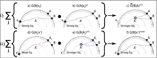
(i) Correlation of the recorded trace at A with that at B for a source at x gives the trace |$\tilde{G}({\bf {B}}|{\bf {A}})_x$| with the virtual diffraction having traveltime denoted by |$\tau _{A^{\prime }B}-\tau _{A^{\prime }A}$|⁠. This arrival time will be the same for all inline source positions that generate CMB diffractions, so stacking |$\sum _j \tilde{G}({\bf {B}}|{\bf {A}})_{x_j}$| will enhance the SNR of the virtual diffraction by |$\sqrt{N_{\rm s}}$|⁠. (ii) The virtual diffraction traces are convolved with the actual diffraction traces and stacked for different station positions to give the supervirtual trace with a SNR enhanced by |$\sqrt{N_{\rm g}}$|⁠. Solid (dashed) rays are associated with positive (negative) traveltimes and the red (blue) ray is associated with the weak (strong) earthquake.

Figure 2.

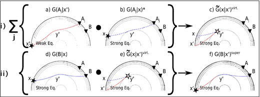
The steps for creating supervirtual diffractions at new virtual stations which were not deployed at the time of the x^′ event. (i) Correlation of the recorded traces at A_j from sources at x and x^′ gives the trace |$\tilde{G}({\bf {x}}|{\bf {x}}^{\prime })_{A_j}=G({\bf {A}}_j|{\bf {x}}^{\prime })G({\bf {A}}_j|{\bf {x}})^*$| with the virtual diffraction having traveltime denoted by |$\tau _{y^{\prime }x^{\prime }}-\tau _{y^{\prime }x}$|⁠. This arrival time will be the same for all inline common receiver positions that records CMB diffractions, so stacking |$\sum _j \tilde{G}({\bf {x}}|{\bf {x}}^{\prime })_{A_j}$| will enhance the SNR of the virtual diffraction by |$\sqrt{N_g}$|⁠. (ii) The stacked virtual trace in (i) is convolved with the raw records (which are of high magnitude) of the event at x to generate supervirtual records at stations B as if they recorded the event at x^′. Solid (dashed) rays are associated with positive (negative) traveltimes and the red (blue) ray is associated with the weak (strong) earthquake.

2.1 Theory

The key idea is to recognize that core-diffracted phases (e.g. Pdiff and Sdiff; Lay et al.1998) graze along the CMB similar to a head-wave refraction. Any receiver that is more than approximately 97° from the epicentre will record this diffraction in the shadow zone of the source, and we will refer to such receivers as having a shadow offset. This ‘shadow offset’ is similar to the term ‘post-critical offset’ for head waves, where refractions are only recorded as first arrivals by receivers that are post-critically offset from the sources. This means that N inline sources beyond a critical shadow distance from the inline pair of recording stations at A and B (see Fig. 1i) will be stationary sources. In this case, stationary sources (Snieder 2004; Schuster 2009) are those where the difference in diffraction traveltimes at stations A and B will be the same for any inline source at a shadow offset because the diffraction path from the source at x_j to A^′ coincides with the raypath for diffraction recorded at either A or B. Therefore, cross-correlating the trace at A with the one at B will yield an arrival at the same correlation time for all shadow-offset sources inline with the receivers. Similar to common midpoint (CMP) stacking of N exploration reflections records (Yilmaz 2001), stacking of the correlated records will enhance the SNR by a factor proportional to |$\sqrt{N}$| for random additive noise. Unlike the CMP method, the SVI procedure has no restrictions on the geometry of the diffraction boundary, it is valid for 3-D structures and no assumption on the background medium is needed for coherent stacking. In the following analysis we will assume that the radiation pattern for any event has been corrected so that the final signals have the same fault plane orientation.

2.1.1 Enhancing the SNR of weak CMB diffractions

To show how SVI can enhance the SNR of CMB diffractions, let us define the vertical component of the earthquake record in the frequency domain¹ as |$G({\bf {A}}|{\bf {x}}_j)=R({\bf {A}}|{\bf {x}}_j){\rm e}^{{\rm i}\omega (\tau _{x_jA^{\prime }}+\tau _{A^{\prime }A})}$| for a recording station at A and an earthquake source at x_j. The earthquake locations are defined as x_j for jϵ[1, 2, …, N_s], as illustrated by the blue rays in Fig. 1(i). Here, |$\tau _{x_jA^{\prime }}+\tau _{A^{\prime }A}$| denotes the traveltime associated with the diffraction ray path from x_j to A, and R(A|x) incorporates the effects of geometrical spreading, transmission effects, the radiation pattern and the source spectrum. A virtual trace (Dong et al.2006) can be created at B by computing the spectral product

\begin{eqnarray} \tilde{G} ({\bf {B}}|{\bf {A}})_{x_j} &=& G({\bf {A}}|{\bf {x}}_j)^*G({\bf {B}}|{\bf {x}}_j) \nonumber\\ &=& R({\bf {A}}|{\bf {x}}_j)^*R({\bf {B}}|{\bf {x}}_j) {\rm e}^{{\rm i} \omega (\tau _{A^{\prime }B}-\tau _{A^{\prime }A})}, \end{eqnarray}

(1)

where |$\tilde{G}({\bf {B}}|{\bf {A}})_{x_j}$| is interpreted as the recording at B of a virtual earthquake located on the refractor at A^′, with this virtual source excited at the advanced time |$-\tau _{A^{\prime }A}$|⁠. Note that the right-hand side phase is independent² of the actual source position x_j and only depends upon the phase difference between diffractions with ray paths denoted by x_jA^′A and x_jA^′B in Fig. 1. Since the ray paths are common over the ray path x_jA^′, then any phase distortions (Choy & Richards 1975) along this common path are eliminated in |$\tilde{G}({\bf B}|{\bf A})_{x_j}$|⁠.

As mentioned earlier, the kinematic phase of |$\tilde{G}({\bf {B}}|{\bf {A}})_{x_j}$| is the same for any inline source³ at a shadow offset, so summing over the source index j gives the coherently stacked virtual trace with an improved SNR for the diffraction arrival:

\begin{eqnarray} G ({\bf {B}}|{\bf {A}})^{{\rm virt}} &=& \sum _{j=1}^{N_s} \tilde{G}({\bf {B}}|{\bf {A}})_{x_j} \nonumber\\ &=& {\rm e}^{j \omega (\tau _{A^{\prime }B}-\tau _{A^{\prime }A})} \sum _{j=1}^{N_s} R({\bf {A}}|{\bf {x}}_j)^* R({\bf {B}}|{\bf {x}}_j). \end{eqnarray}

(2)

To restore this virtual record, such that it kinematically resembles one from the actual earthquake, we must convolve its time domain representation with a recorded arrival such as the one associated with the red ray in Fig. 1(ii). In the frequency domain, Fig. 1(ii) shows that this is equivalent to the product of the G(A_j|x^′) trace with the virtual record G(B|A_j)^virt.

In the time domain, the product G(A_j|x′)G(B|A_j)^virt for a specified event location x^′ and shadow receiver location A_j, represents a trace with the same arrival time for any shadow-offset receivers |$\bf B$| and A_j. Therefore, stacking over station positions A_j for jϵ[1, 2, …, N_g] gives the supervirtual trace G(B|x′)^super

\begin{eqnarray} G({\bf {B}}|{\bf {x}}^{\prime })^{{\rm super}} &=& \sum _{j=1}^{N_g} G({\bf {A}}_j|{\bf {x}}^{\prime }) G({\bf {B}}|{\bf {A}}_j)^{{\rm virt}} . \end{eqnarray}

(3)

For normally distributed additive white noise the SNR enhancement should be |$\sqrt{N_g}$|⁠, where N_g is the number of common receivers for the sources at x^′ and x_j.

2.1.2 Creating new virtual recording stations

Fig. 2 illustrates how SVI can also be used to create virtual records at stations not deployed during the time of the earthquake at x^′. The requirement is that the station at A_j records diffraction arrivals from two earthquakes, one at |$\bf x$| and the other at |$\bf x^{\prime }$|⁠. The earthquake at |$\bf x^{\prime }$| can be weak, but the other one at |$\bf x$| must be strong with a high SNR for the CMB event. Now, the stacked virtual trace

\begin{eqnarray} G({\bf {x}}|{\bf {x}}^{\prime })^{{\rm virt}}&=& \sum _j G({\bf A}_j|{\bf x^{\prime }})G({\bf A}_j|{\bf x})^* \nonumber\\ &=& {\rm e}^{{\rm i}\omega (\tau _{x^{\prime }y^{\prime }}-\tau _{xy^{\prime }})}\sum _{j} R({\bf {A}}_j|{\bf {x}}^{\prime }) R({\bf {A}}_j|{\bf {x}})^*\nonumber\\ &=& {\rm e}^{{\rm i}\omega (\tau _{x^{\prime }y^{\prime }}-\tau _{xy^{\prime }})}R({\bf {x}}|{\bf {x}}^{\prime })^{{\rm virt}}, \end{eqnarray}

(4)

is generated by stacking over different recording stations A_j as illustrated in Fig. 2(i). The result is a virtual trace G(x|x′)^virt with an enhanced SNR of |$\sqrt{N_g}$|⁠, where N_g is the number of paired receiver stations for the two events.

Next, we assume that the recording stations have then been moved to the locations around B in Fig. 2(ii); the goal is to create virtual records at B as if they were generated by the old earthquake at x^′. This can be accomplished by assuming that a strong event occurs at the location x to give the new record |$G({\bf {B}}|{\bf {x}})=R({\bf {B}}|{\bf {x}}){\rm e}^{{\rm i}\omega (\tau _{xy^{\prime }}+\tau _{y^{\prime }B})}$|⁠. From eq. (4) and Fig. 2(ii), we can form the product

\begin{eqnarray} G({\bf {B}}|{\bf {x}}^{\prime })^{{\rm super}} &=&G({\bf {B}}|{\bf {x}})G({\bf {x}}|{\bf {x}}^{\prime })^{{\rm virt}} \nonumber\\ &=&R({\bf {B}}|{\bf {x}}) R({\bf {x}}|{\bf {x}}^{\prime })^{{\rm virt}} {\rm e}^{{\rm i} \omega (\tau _{xy^{\prime }}+\tau _{y^{\prime }B})}{\rm e}^{{\rm i} \omega (\tau _{x^{\prime }y^{\prime }}-\tau _{xy^{\prime }})} \nonumber\\ &=&R({\bf {B}}|{\bf {x}}) R({\bf {x}}|{\bf {x}}^{\prime })^{{\rm virt}}{\rm e}^{{\rm i} \omega (\tau _{x^{\prime }y^{\prime }}+\tau _{y^{\prime }B})}, \end{eqnarray}

(5)

to give the supervirtual record G(B|x′)^super at B as if it were generated by the old earthquake at x^′. The key assumption is that the strong earthquake at |$\bf x$| repeated itself after the deployment of the newly activated station at |$\bf B$|⁠. Even a strong earthquake near the vicinity of x can be used instead of one exactly at x, as this would only give rise to a constant timing error for all the traces in the virtual event gather G(B|x′)^super.

A practical implementation of eq. (5) is to simply pick the time |$\tau _{x^{\prime }y^{\prime }}-\tau _{xy^{\prime }}$| associated with the diffraction arrival in the G(x|x′)^virt record, and apply this as a time-shift to the G(B|x) trace. This is a viable strategy because the SNR of the G(x|x′)^virt trace (see eq. 4) should be large for a sufficient number of recording stations. This is the strategy first suggested by Dong et al. (2006) and will be used for our synthetic and field data examples. However, this picking can be ambiguous due to wavelet distortion if the focal mechanisms of the events at x and x^′ are different and not corrected, so this can lead to a constant time-shift error in the generated supervirtual traces. The only value in creating a wider array of virtual recording stations for a single earthquake location is that it can reduce the acquisition footprint in a traveltime tomogram. No new information about the subsurface is contained in these virtual traces in the extended array.

2.2 Processing work-flow

The work-flow for processing the teleseismic data consists of the following four steps in an extended array associated with Fig. 1. To create virtual records, the last two steps should be replaced by those associated with Fig. 2.

• Teleseismic records computed by an elastic modelling code or downloaded from online databases are first processed using basic procedures such as tapering, demeaning, re-sampling and bandpass filtering (typically 0.008–2 Hz) followed by normalization.

• For the field data, the instrument response at each station is used to deconvolve the records. After rotating seismogram components to the (Z, R, T) system, a 400 s time window is applied around the P-wave diffractions in the Z-component and S-wave diffractions in the T- or R-component records. Windowing must be used because it helps to reduce the interference between the diffractions and other arrivals in the earthquake records due to the cross-correlation and convolution operations.

• Eq. (2) is replaced by the following equation:

  \begin{eqnarray} G({\bf {B}}|{\bf {A}})^{{\rm virt}}&=& \sum _j \frac{G({\bf {B}}|{\bf {x}}_j)G({\bf {A}}|{\bf {x}}_j)^*}{|G({\bf {B}}|{\bf {x}}_j)|^2+\epsilon }, \end{eqnarray}

  (6)

  where ϵ is a small positive damping coefficient. The motivation is that this deconvolution procedure partly corrects for the source wavelet distortions due to correlation (Vasconcelos & Snieder 2008). Virtual records with the SNR enhanced by |$O(\sqrt{N_{\rm s}})$| are generated using eq. (6), where N_s is the number of strong events in the summation over j. Generally these events can be of high magnitude so we have virtual traces with high SNR even if N_s is small.

• The virtual records are then convolved with the corresponding filtered records of the weak arrival G(A_j|x^′) excited at x^′ in Fig. 1(ii); these earthquakes at x^′ can now be of low magnitude because they are stacked over many receiver positions to get G(B|x′)^super with a high SNR. The key benefit here is that the SNR of weak earthquakes can now be boosted and therefore increase the number of useful teleseisms in a catalogue.

3 SYNTHETIC EXAMPLES

Synthetic seismograms are generated using the axisymmetric spectral-element code AxiSEM (Nissen-Meyer et al.2008) with the PREM background model (Dziewonski & Anderson 1981). This method efficiently solves the 3-D equations of motion for spherically symmetric (or axisymmetric) background models in a 2-D computational domain, and can thus accommodate high-frequency wavefields (up to 1 Hz). The data set consists of three earthquake gathers with 81 receivers evenly spaced between 100° and 180°; events have the same epicentre but are located at different depths (15, 40 and 70 km) and have different source periods as well as radiation patterns (listed in Table 1). We did not correct the radiation pattern prior to processing. The time sampling is 0.2 s, and all records are 1500 s long such that P-wave diffractions can be observed at all relevant distances.

Table 1.

Synthetic data set.

Event no.	Depth (km)	Dominant source period (s)	Radiation pattern
1	15	10	Vertical vector dipole
2	40	10	Vertical vector dipole
3	70	5	Vertical dip-slip

3.1 Enhancing the SNR of weak earthquakes

Records for the event at a 70 km depth are plotted in Fig. 3(a) with additive band-limited (0.001–2 Hz) white random noise so that the SNR is as low as 0.03. We consider such noisy traces to result from a low-magnitude earthquake. The records of other earthquakes have a relatively high SNR corresponding to a large magnitude (>6.5) event as plotted in Fig. 3(b). Fig. 3(d) is the result of inserting the noisy synthetic teleseisms into eq. (2) to create virtual records with a high SNR, and then convolving these virtual traces with the strong records (see eq. 3) to obtain the supervirtual traces. Since there are 80 recording stations we should see a SNR improvement proportional to |$\sqrt{80}\approx 9$|⁠, which is consistent with the clean traces in Fig. 3(d) compared to the original noisy records in Fig. 3(a). Most of the traveltimes of CMB diffractions in Fig. 3(d) can now be picked and they agree with the actual arrival times in Fig. 3(c).

Figure 3.

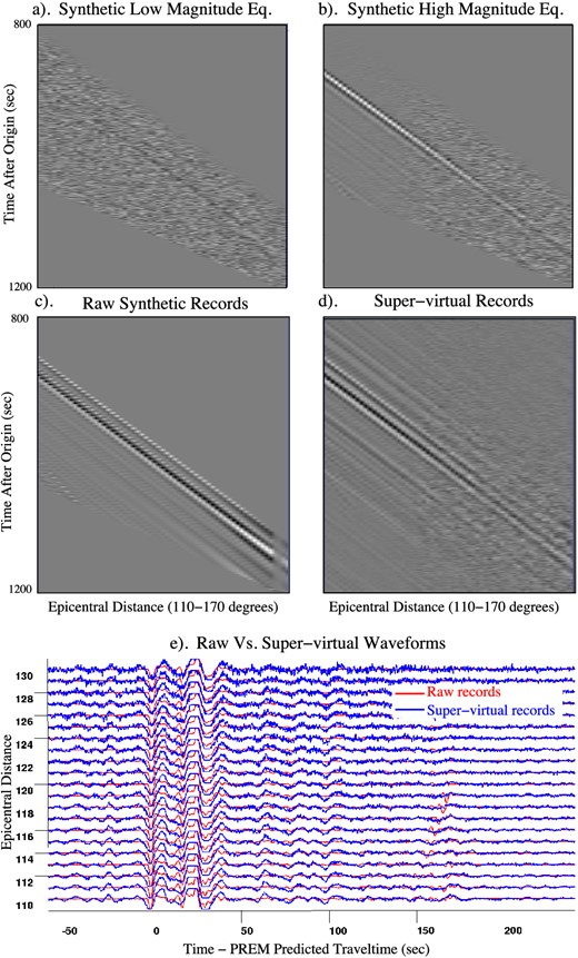
(a) Windowed R-component synthetic records of the event at 70 km depth after adding random noise where the SNR is as low as 0.03. The associated earthquake represents a low-magnitude event whose records are to be enhanced so that the diffractions can be picked. (b) Same as (a) except the event depth is at 15 km and it is a high magnitude event. (c) Raw synthetic records of the low magnitude event in (a) before adding random noise. (d) Supervirtual records of the low magnitude event in (a) showing enhanced P-diff arrivals. (e) Comparing supervirtual and actual records of the low magnitude event in both wave-shape and timing. The seismograms are sorted by epicentral distance and shifted in time by the PREM predicted arrival time.

In order to test the effect of only pulse distortions (Choy & Richards 1975) in the diffracted phases, we regenerated the supervirtual records without adding random noise to any of the raw records. The traveltimes of the P-diff phases in these supervirtual records are hand-picked and are compared with those in the raw records (Fig. 3c). The difference in the picked traveltimes as a function of epicentral distance is plotted in Fig. 4 where no significant error dependence on the epicentral distance can be seen. The time period of the maximum frequency in the spectrum is approximately 8 s, and the mean traveltime difference is about 1/16th of the period, that is, in the same regime as the picking error. Thus, the effect of pulse distortions on the traveltimes can be neglected for our results.

Figure 4.

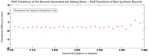
Picked P-diff traveltime differences between supervirtual records (generated without adding random noise) and raw synthetic records. The mean traveltime error of about 0.5 s is 1/16th the minimum period of 8 s for the source wavelet.

3.2 Generating new recordings

We assume a weak event at 70 km depth recorded at stations deployed between 130° and 170° from the epicentre, as shown on the right-hand side of Fig. 5; this earthquake will be denoted as event A. The goal is to create virtual records of event A at stations between 110° and 130° from other events recorded at stations with an epicentral range between 110° and 170°.⁴ This goal is similar to that proposed in Curtis et al. (2012), except that we use earthquake-generated diffracted body waves rather than ambient-noise generated surface waves. Consequently, the earthquake source spectrum is maintained while the ambient noise sources limit those application to the (often narrower) noise spectra.

Figure 5.

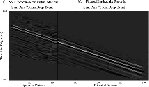
(a) Kinematically accurate supervirtual records at new virtual stations between 110° and 130° which were not deployed during the 70-km-deep event but are generated using the method illustrated in Fig. 2. (b) Synthetic filtered R-component records from the stations which record the 70-km-deep event.

We will use the procedure illustrated in Fig. 2 to create these virtual records, where the input data consists of two data sets:

• Records of weak event A only recorded between 130° and 170° distance for the 70-km-deep event.

• Records of a strong 15-km-deep earthquake, labelled as event B, recorded by stations between 110° and 170°.

As illustrated in Fig. 2(i), the stacked virtual trace is generated from the 70-km-deep and the 15-km-deep events to pick the peaked arrival corresponding to the time |$\tau _{y^{\prime }x^{\prime }}-\tau _{y^{\prime }x}$|⁠. By using this picked arrival time, a time shift is then applied to the filtered records of the 15-km-deep event to obtain the supervirtual records of the 70-km-deep event as if they were recorded at the new virtual stations between 110° and 130°. This time-shifting operation is equivalent to the convolution step in Fig. 2(ii), and the supervirtual records generated by this method are plotted on the left-hand side of Fig. 5. The traveltimes of the CMB diffractions in these supervirtual records are in excellent agreement with the theoretical traveltimes.

4 APPLICATION TO RECORDED EARTHQUAKE DATA

The SNR enhancement of CMB diffractions and the creation of virtual traces will be tested with Indonesian earthquakes recorded by USArray stations, with the epicentres listed in Table 2 and plotted in Fig. 6. For the field data, the recording stations chosen along with the epicentres of the earthquakes are along or within a wavelength of the same great circle, that is, a Fresnel ribbon. To account for stations within a Fresnel ribbon, we select an azimuth/backazimuth span of 10° in our numerical examples.

Figure 6.

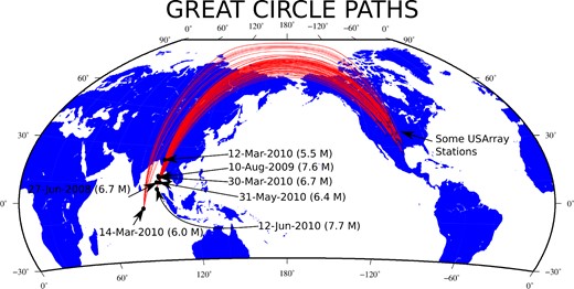
Epicentre locations of events listed in Table 2. Great circle paths are drawn to some of the USArray stations. Before SVI processing the stations and events should be selected such that they are located on the Fresnel ribbon of the same great circle.

Table 2.

Locations of earthquakes.

No.	Date	Latitude	Longitude	Depth (km)	Magnitude
1	2009 August 10	14.01°N	092.92°E	33.1	7.6
2	2010 March 12	23.06°N	094.62°E	102.0	5.5
3	2010 March 30	13.66°N	092.83°E	34.0	6.7
4	2010 June 12	07.70°N	091.97°E	35.0	7.7
5	2010 May 31	11.11°N	093.69°E	127.0	6.4
6	2010 March 14	02.76°S	083.67°E	10.0	6.0
7	2008 June 27	11.03°N	091.90°E	35.0	6.7

4.1 Enhancing the SNR of weak earthquakes

Broad-band records are readily available from seismic databases such as IRIS. We downloaded data for different U.S. transportable array (TA) stations from IRIS, and deconvolved them with the instrument response of the corresponding station. After rotation, the vertical (Z) and transverse (T) component data are used, respectively, to enhance the P- and S-wave diffractions from the CMB. A bandpass filter (0.008–0.12 Hz) is applied to all of the low-magnitude event records, and a filter of 0.008–2 Hz is applied to the other earthquake records which are of relatively higher magnitude. For each event the stations are selected so that their epicentral distances are greater than 110°. The station records of several high-magnitude earthquakes listed in the Table 2 are plotted in Fig. 7. The stations are sorted with increasing epicentral distance on the x-axis and their records show distinct P-diff arrivals.

Figure 7.

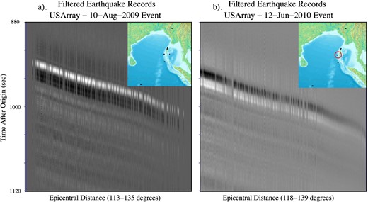
Plots showing filtered transportable array (TA) records of different high magnitude earthquakes where the station index on the x-axis is the same. The record of a particular station is left blank if it did not record the event. The stations are sorted with increasing epicentral distance on the x-axis. The x-axis is not scaled but its range is indicated. (a) Time windowed and filtered (0.008–2 Hz) Z-component records for the 2009 August 10 earthquake which is circled red on the map. (b) Same as (a) but for the 2010 June 12 event.

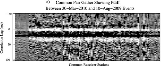
Fig. 8 displays the common pair gather⁵ (CPG) of traces, where any correlogram is formed by correlating a recorded trace at A_j from the 2010 March 30 event with a trace recorded at A_j for the 2009 August 10 event (see Fig. 2i). A 800–1200 s time window to the Z-component records is applied prior to correlation. Now we show the results of SVI processing on both intermediate and weak magnitude events as described below.

• Intermediate magnitude 2010 May 31 event: Actual T-component records of this event are plotted in Fig. 9(a). The SNR of the S-diff arrival is boosted as shown in the SVI records of Fig. 9(b). As a sanity check, note other coherent events (green arrow in actual data panel) are suppressed during SVI processing since they have different moveout.

• Weak magnitude 2010 Mar 12 event: An event with an epicentre closer to the USArray stations compared to high magnitude event epicentres is chosen to test the method. Figs 10(a) and 11(a) show, respectively, the noisy Z- and T-component records of this event. The corresponding SVI records in Figs 10(b) and 11(b) show enhanced P-diff and S-diff arrivals.

• Weak magnitude 2010 March 14 event: The epicentre of this event is far from the USArray stations compared to other high magnitude event epicentres used in the processing, where the Z-component records before and after SVI processing are plotted in Fig. 12.

Figure 8.

A common pair gather generated using cross-correlation as shown in Fig. 2. Each virtual trace, |$\tilde{G}({\bf {x}}|{\bf {x}}^{\prime })_{A_j}$| is generated for different positions of the station A_j (see eq. 1).

Figure 9.

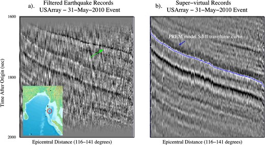
T-component records of a low magnitude (2010 May 31) event which is circled red in the map. The stations are sorted with increasing epicentral distance on the x-axis. The x-axis is not scaled but its range is indicated. (a) Filtered (0.01–0.12 Hz) records at different stations. (b) Supervirtual records corresponding to filtered records in (a) showing enhanced SNR.

Figure 10.

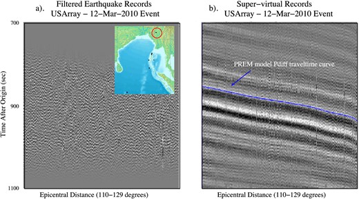
Z-component records of a low magnitude (2010 March 12) event which is circled red in the map. The stations are sorted with increasing epicentral distance on the x-axis. The x-axis is not scaled but its range is indicated. (a) Filtered (0.008–0.12 Hz) records at different stations. (b) Supervirtual records corresponding to filtered records in (a) showing enhanced SNR. The solid blue line indicates the calculated P-diff traveltime in the case of the PREM model, and the traveltime at the first receiver is 856.36 s.

Figure 11.

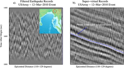
T-component records of a low-magnitude (2010 March 12) event which is circled red in the map. The stations are sorted with increasing epicentral distance on the x-axis. The x-axis is not scaled but its range is indicated. (a) Filtered (0.008–0.12 Hz) records at different stations. (b) Supervirtual records and corresponding to filtered records in (a) showing enhanced SNR. The solid blue line indicates the calculated S-diff traveltime associated with the PREM model, the traveltime at the first receiver is 1583 s.

Figure 12.

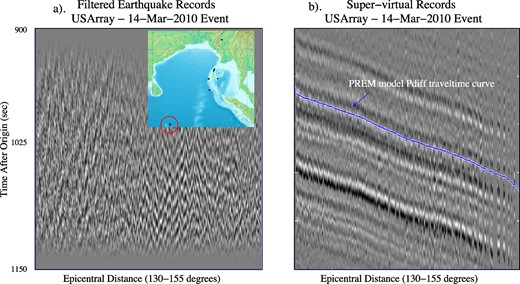
Z-component records of 2010 March 14 event which are of low magnitude and circled red on the map. The stations are sorted with increasing epicentral distance on the x-axis. The x-axis is not scaled but its range is indicated. (a) Filtered (0.008–0.12 Hz) records at different stations. (b) Supervirtual records corresponding to filtered records in (a) showing enhanced SNR.

In all the above cases approximately 200 supervirtual traces are stacked after convolution (see Fig. 1ii), such that the SNR should be increased by a factor of about 14 (assuming additive white noise).

4.2 Generating new recordings

The procedure illustrated in Fig. 2 is used to create virtual records at stations that were not deployed during the 2008 June 27 event. As shown in the Fig. 2(i), the stacked virtual trace is generated from the 2008 June 27 and the 2010 June 12 events to pick the peaked arrival corresponding to the time |$\tau _{y^{\prime }x^{\prime }}-\tau _{y^{\prime }x}$|⁠. A time shift is then applied to the filtered records of the 2010 June 12 event to obtain the supervirtual records of the 2008 June 27 event as if they were recorded at the new virtual stations. This time-shifting operation is equivalent to the convolution step in Fig. 2(ii). The supervirtual records generated by this method are plotted in Fig. 13, and the traveltimes of the CMB diffractions agree well with those predicted from the PREM model.

Figure 13.

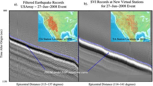
(a) Filtered Z-component records from the stations which were deployed at the time of the 2008 June 27 earthquake whose positions are plotted on the map. (b) Supervirtual records at new virtual stations which were not deployed during the 2008 June 27 event but are generated using the method illustrated in Fig. 2. The new virtual station positions are also plotted on the map. The stations are sorted with increasing epicentral distance on the x-axis. The x-axis is not scaled but its range is indicated.

5 RANDOM NOISE TEST

The input records to the supervirtual algorithm described in the previous sections are both from weak and strong magnitude events (the weak magnitude records have the appearance of noise). If the weak events have sufficiently low SNR then the resulting supervirtual traces might contain a partial imprint of the strong event. That is, the moveout (or relative time-shift between the diffractions recorded at two stations) information seen in the supervirtual records is from the strong event. The valuable information in the supervirtual records is the traveltime for the diffracted energy to reach at least one of the stations from the weak event focus. These diffractions from the weak event illuminate the extra ray path (as illustrated in Fig. 14 ) which was not previously illuminated by the strong event.

Figure 14.

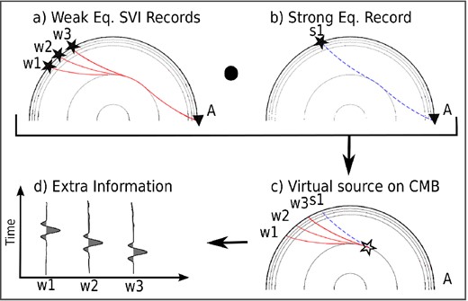
(a) Enhanced SVI records at station A for the weak events (W1, W2 and W3). (b) Record at A due to a strong event (S1). (c) Cross-correlation results in a virtual source on the CMB. (d) These virtual records contain new information as they illuminate new areas along the CMB not traversed by the strong event's ray path.

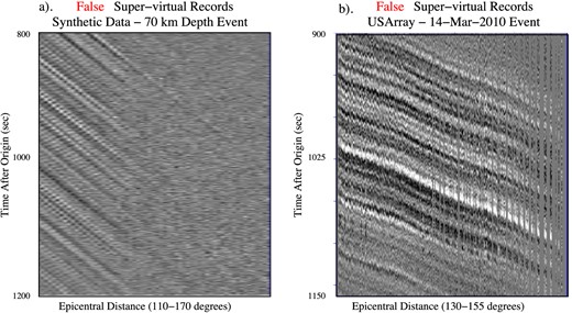
In this section, we test the imprint of the strong event on the supervirtual records by replacing the weak event records with white noise prior to SVI processing. These false supervirtual records are generated using both synthetic and USArray records and are plotted in Fig. 15. The imprint of the strong events is evident as coherent events with correct moveout. However these coherent events focus at the correct traveltime only if the actual weak event records are used. For example, see the true supervirtual records in Figs 3(d) and 12(b). Also, the synthetic record plots in Fig. 16 show the difference between these true and false supervirtual records. We recommend that the application of the method to real earthquake records should be tested for sensitivity to the imprint of the strong event record by the following tests.

• Replace the weak event records by random noise and generate the SVI traces.

• Shift the weak event records by random time-shifts and rerun the code to generate SVI traces.

Figure 15.

False supervirtual records are generated by replacing the weak event records with white noise prior to SVI processing. (a) Same as Fig. 3(d) but the input weak event records are replaced by random noise. (b) Same as Fig. 12(b) but the input weak event records are replaced by random noise.

Figure 16.

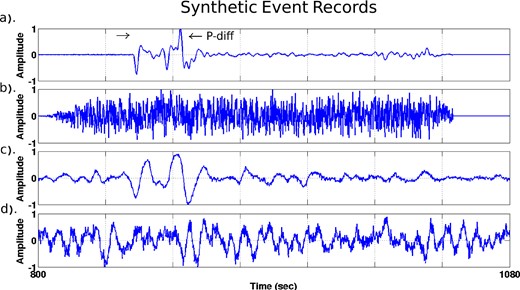
Synthetic wiggle plots of a R-component record at an epicentral distance of 110° corresponding to the 70-km-deep weak event. (a) Raw record corresponding to Fig. 3(c). (b) Same as (a) but after adding random noise. (c) Output record after SVI processing showing enhanced SNR. (d) False SVI record of random noise test (first record of Fig. 15a).

In both these cases the coherent signal in the resultant supervirtual records should fade out depending on the time window length of the input records. Larger time windows (compared to the wavelength) should result in better cancellation.

6 CONCLUSIONS

SVI is applied to synthetic earthquake data and to teleseismic earthquake records recorded by USArray. Results with both synthetic traces and field data show a noticeable SNR improvement for traces with CMB diffractions for both P and S waves. Indonesian earthquakes with a magnitude between 5.5 and 6.2 did not show clear CMB diffractions, but after SVI processing showed clearly identifiable diffraction arrivals. This suggests that many of the weaker and unusable earthquakes associated with the Indonesian subduction zone and recorded by USArray can be enhanced for analysis of CMB diffractions. More generally, the SNR of weak teleseismic recordings of CMB diffractions and mantle refractions throughout the world can now be enhanced by SVI to greatly expand the catalogue of useful earthquake records. This invigorated data can significantly enlarge the number of traveltimes and waveforms used for tomographic inversion and migration of CMB and D^′′ data, and therefore might provide novel information about the Earth's deep interior.

We also showed that SVI can generate virtual recordings of an earthquake at stations not deployed during the time of the earthquake. This means that transient arrays such as USArray can extend the aperture of one recorded earthquake from the West coast to the East coast, even though the teleseism might have only been recorded during the West coast deployment. This assumes that the arrivals of interest are those of CMB diffractions or refractions from the mantle and/or core. The only identifiable benefit here is that the extended array data set can reduce the acquisition footprint in the traveltime tomogram.

Two limitations of this method are that the sources and receivers must be mostly inline along the same great circle path, and the radiation pattern from different fault orientations must be corrected prior to combining data from different earthquakes. Another limitation is that the absolute waveform accuracy of the SVI events is not preserved. However, the relative change in amplitude in a common earthquake gather should be preserved, which can be a useful diagnostic of the CMB boundary. As a cautionary measure, tests similar to the random noise test should be carried out for assessing the sensitivity to imprinting the strong event record onto the SVI record. Future work should apply this methodology to refraction arrivals in the mantle and the core. This methodology can also be applied to surface wave arrivals, because all sources that generate surface waves are stationary sources as long as they are approximately inline with the receivers. This especially applies to multi-orbit and high-frequency surface waves which quickly loose detectable amplitudes with respect to the noise level.

Data from the TA network were made freely available as part of the EarthScope USArray facility, operated by Incorporated Research Institutions for Seismology (IRIS) and supported by the National Science Foundation, under Cooperative Agreements EAR-0323309, EAR-0323311, EAR-0733069. We thank the KAUST Supercomputing Lab for their support to this project and use of the Shaheen computer. We also acknowledge the support from the KAUST CRG grant and the CSIM sponsors (http://csim.kaust.edu.sa). TNM thanks the Petaquake project of the Swiss HP2C initiative for financial support. The authors are grateful to anonymous reviewers for their insightful criticism that helped to improve the manuscript.

*

Now at: Department of Earth Sciences, University of Oxford, South Parks Road, Oxford OX1 3AN, UK.

1

The angular frequency variable ω is silent in the band-limited Green's function notation.

2

This assumes that the spectral product of the geometric spreading terms is real.

3

This assumes that the radiation patterns and source signatures of each source have been normalized to be the same for any earthquake.

4

Recording up to 170° is only theoretically possibly for diffracted waves, in practice scattering and attenuation will make this completely infeasible to observe even with minimal noise. However, in synthetic scenarios for purely elastic spherically symmetric media they can be observed.

5

A CPG is a gather of virtual traces created by cross-correlating two traces recorded at A_j (see Fig. 2i) and generated by a common pair of earthquakes (Dong et al.2006). A CPG can also be generated by correlating traces recorded by a common pair of receivers generated by different sources.