Full sphere hydrodynamic and dynamo benchmarks

Abstract

Convection in planetary cores can generate fluid flow and magnetic fields, and a number of sophisticated codes exist to simulate the dynamic behaviour of such systems. We report on the first community activity to compare numerical results of computer codes designed to calculate fluid flow within a whole sphere. The flows are incompressible and rapidly rotating and the forcing of the flow is either due to thermal convection or due to moving boundaries. All problems defined have solutions that allow easy comparison, since they are either steady, slowly drifting or perfectly periodic. The first two benchmarks are defined based on uniform internal heating within the sphere under the Boussinesq approximation with boundary conditions that are uniform in temperature and stress-free for the flow. Benchmark 1 is purely hydrodynamic, and has a drifting solution. Benchmark 2 is a magnetohydrodynamic benchmark that can generate oscillatory, purely periodic, flows and magnetic fields. In contrast, Benchmark 3 is a hydrodynamic rotating bubble benchmark using no slip boundary conditions that has a stationary solution. Results from a variety of types of code are reported, including codes that are fully spectral (based on spherical harmonic expansions in angular coordinates and polynomial expansions in radius), mixed spectral and finite difference, finite volume, finite element and also a mixed Fourier–finite element code. There is good agreement between codes. It is found that in Benchmarks 1 and 2, the approximation of a whole sphere problem by a domain that is a spherical shell (a sphere possessing an inner core) does not represent an adequate approximation to the system, since the results differ from whole sphere results.

Numerical solutions, Non-linear differential equations, Dynamo: theories and simulations, Planetary interiors

1 INTRODUCTION

The predominant theory for the generation mechanism of the Earth's magnetic field is that of magnetic field generation by thermal and compositional convection, creating the so-called self-excited dynamo mechanism. Beginning with the first 3-D self-consistent Boussinesq models of thermal convection (Glatzmaier & Roberts 1995; Kageyama et al.1995), there has been burgeoning interest in numerical solutions to the underlying equations of momentum conservation, magnetic field generation and heat transfer. Given the complexity and non-linearity of the physics, it has been of importance to verify that the codes used correctly calculate solutions to the underlying equations, and also to provide simple solutions that allow newly developed codes to be checked for accuracy. It is now over 11 yr since the undoubtedly successful numerical dynamo benchmark exercise of Christensen et al. (2001); Christensen et al. (2009), hereinafter B1. This benchmark exercise was set in the geometry of a spherical shell, with convection driven by a temperature difference between an inner core and the outer boundary of the spherical shell. In this respect, the computational domain is similar to that of the Earth, possessing as it does a small inner core. Three different benchmarks were devised, the first being purely thermal convection, and the second and third being dynamos (supporting magnetic fields). The latter two benchmarks differed in the treatment of the inner core: in one case the inner core was taken to be electrically insulating and fixed in the rotating frame, and in the other case the core was taken to be electrically conducting and free to rotate in response to torques that are applied to it, arising from the convection in the outer core. Central to these benchmarks was the fact that all of them possessed simple solutions, in the form of steadily drifting convection. As a result, energies are constant and, together with other diagnostics, these provide very clear solutions that could be reproduced by different numerical techniques. A measure of the success of this exercise is given by the fact that it has been used by numerous groups to check their codes.

The present benchmarking exercise is one of two brethren designed to broaden the scope of the original B1 and to provide further accurate solutions for a new generation of computer codes. The associated exercise by Jackson et al. (2013) is also set in a spherical shell as in B1; it is similar to B1 but has been designed to be particularly amenable to computer codes based on local (rather than spectral or global) descriptions of the temperature, magnetic and velocity fields. Thus, that benchmark allows comprehensive checking of finite element, finite volume and similar computer codes, as a result of the implementation of a local rather than global magnetic boundary condition. This paper treats a similar situation to B1 but differs in the removal of the inner core, and thus treats only a whole sphere. Flows in the first two benchmarks thus defined are driven by thermal convection, again under the Boussinesq approximation, and in the third by a boundary forcing. There are two reasons for defining benchmarks set in the whole sphere rather than the spherical shell. First, the whole sphere represents a canonical problem, surely a simpler geometry than the shell. There is one less degree of freedom, since the aspect ratio of the shell is no longer a defined parameter. Secondly, in the context of rapidly rotating fluid dynamics, there is likely to be a simplification in the flow structures generated because of the absence of an inner core. It is well known that the dynamics of rapidly rotating systems is dominated by the Coriolis force, thus leading to the Proudman–Taylor constraint, the alignment of flow structures with the rotation (z) axis. In a spherical shell when viscosity is reduced, as one moves from outside the so-called tangent cylinder (the cylinder that just encloses the inner core) to inside the tangent cylinder, a jump is present in the length of a column in the z-direction. Hence, there is the possibility of the need to resolve very fine shear layers in this region; for a recent discussion, see Livermore & Hollerbach (2012). The presence of very fine structures that need to be resolved can have very deleterious effects on a numerical method, particularly a spectral method based on spherical harmonics (again, for a discussion, see Livermore 2012). Thus, the choice of a full sphere is likely to be advantageous in the limit in which the viscosity is dropped to insignificant levels.

We note in passing that the whole sphere geometry is particularly relevant to the generation of magnetic fields in the early Earth, prior to the formation of the inner core. In this time period, the convection in the core was driven by secular cooling (and possibly internal heating), and this is precisely the scenario studied here in Benchmarks 1 and 2. Associated with this geometry is a possible numerical obstacle that has perhaps been responsible for the dearth of full-sphere calculations in the literature. Working in a spherical coordinate system (r, θ, ϕ), that is presumably convenient from the point of view of boundary conditions, the presence of the origin of the spherical coordinate system (r = 0) in the integration domain leads to additional numerical challenges. The results presented here show that the employed methods are able to correctly handle this singularity in coordinates.

The Benchmarks 1 and 2 set up here differ from those of B1 in their use of stress-free boundary conditions, rather than non-slip conditions. This arose purely as a result of our survey of parameter space while searching for whole-sphere dynamos that possess simple solutions with clear diagnostics suitable for a benchmark. In performing this survey, we did not find a dynamo that had a steady character similar to that in B1; this is not to say that one does not exist. The dynamo solution in Benchmark 2 shows an exact periodic character with energy conversion between kinetic and magnetic forms. It thus allows very precise comparison. The use of stress-free boundaries can cause problems with angular momentum conservation (see the discussion in Jones et al.2011), but these were handled gracefully in the solutions we report.

We mention in passing the other benchmarks that have recently been provided to the community. A new benchmark for anelastic convection has recently been described by Jones et al. (2011) and already used as a comparison for the newly developed code of Zhan et al. (2012). This benchmark again is set in a spherical shell, but has a background state with a very large change in density across the shell. Three solutions are again compared, the first two (pure thermal convection and dynamo action, respectively) possessing simple drifting solutions with very precise diagnostics. A solar mean field benchmark has also recently been provided by Jouve et al. (2008).

The layout of the paper is as follows: in Section 2, we describe the physical problems to be addressed. Benchmarks 1 and 2 are driven by internal heating and Benchmark 3 by boundary forcing. In Section 3, we give a brief overview of the different numerical methods that have been employed by the different contributing teams. In Section 4, we present and discuss the results from the different codes.

2 TEST CASES

Three benchmarks for incompressible flows in a rapidly rotating whole sphere are considered. The first two test problems, Benchmarks 1 and 2, are subject to the thermal forcing of a homogeneous distribution of heat sources in the volume. Benchmark 1 is a purely hydrodynamic problem while Benchmark 2 consists of a self-sustained dynamo problem. Benchmark 3 extends the scope of these test cases by considering the mechanical forcing induced by moving boundaries. In all cases, the system consists of a whole sphere of radius r_o, filled with a fluid of density ρ and a kinematic viscosity ν. The system rotates at a rotation rate Ω. The fluid motion is described by the velocity field |${\bf u}$| and, for Benchmarks 1 and 2, the temperature field is denoted by T.

2.1 Benchmark 1: thermal convection

Benchmark 1 is a purely hydrodynamic problem with the motion of the fluid described in the reference frame of the mantle. The system is described within the frame of the Boussinesq approximation, neglecting the density fluctuations except for the ones responsible for the buoyancy. Under the action of a gravitational field

\begin{equation} {\bf g} = {g} \frac{{\bf r}}{r_o} \end{equation}

(1)

and in the presence of a homogeneous heat source distribution S, the basic state is given by

\begin{equation} T_b = \frac{\beta }{2}\left(r_o^2 - r^2\right) \end{equation}

(2)

with β = S/3κ, where κ is the thermal diffusivity. The equations are non-dimensionalized using the radius r_o as length scale, the diffusion time |$r_o^2/\nu$| as timescale and |$\beta r_o^2$| as temperature scale. The three non-dimensional parameters are chosen to be the Ekman number E

\begin{equation} E = \frac{\nu }{2\Omega r_o^2}, \end{equation}

(3)

the Prandtl number Pr

\begin{equation} Pr = \frac{\nu }{\kappa } \end{equation}

(4)

and the modified Rayleigh number Ra

\begin{equation} Ra = \frac{g\alpha \beta r_o^3}{2\Omega \kappa }, \end{equation}

(5)

with α the thermal expansion coefficient. The motion of the fluid is then described by the non-dimensional Navier–Stokes equation and the incompressibility condition for the velocity field |${\bf u}$|

\begin{eqnarray} E\left( \partial _t - \nabla ^2 \right) {\bf u} = & E {\bf u}\wedge \left( \nabla \wedge {\bf u} \right) + Ra T\! {\bf r} - {\skew 3\hat{ {\bf z}}}\wedge {\bf u} - \nabla \pi , \end{eqnarray}

(6)

\begin{eqnarray} \nabla \cdot {\bf u} = & 0 \end{eqnarray}

(7)

with |${\skew 3\hat{ {\bf z}}}$| being the rotation axis. The evolution of the temperature T is described by the non-dimensional transport equation

\begin{equation} \left(P_r\partial _t - \nabla ^2\right)T = S - P_r {\bf u}\cdot \nabla T, \end{equation}

(8)

and the non-dimensional basic state is given by

\begin{equation} T_b = \frac{1}{2}\left(1-r^2\right). \end{equation}

(9)

The system is subject to stress-free and impenetrability mechanical boundary conditions and a fixed temperature at the outer boundary. Thus, while the radial velocity component has to vanish, a non-zero horizontal velocity component is possible at the boundary.

The benchmark solution is obtained for an Ekman number E = 3 × 10⁻⁴, a Prandtl number Pr = 1, a Rayleigh number Ra = 95 and a source term S = 3. This choice of parameters is close to the critical values for the onset of convection. More than one solution exists for this choice of parameters. To select the right solution branch, the following initial condition should be used for the temperature field:

\begin{eqnarray} T =\frac{1}{2}\left(1 - r^2\right) + \frac{10^{-5}}{8}\sqrt{\frac{35}{\pi }}r^3\left(1-r^2\right)\left(\cos 3\phi +\sin 3\phi \right)\sin ^3\theta .\nonumber\\ \end{eqnarray}

(10)

For the sake of completeness, the second solution branch might be selected by replacing the spherical harmonic perturbation of degree and order 3 by a spherical harmonic perturbation of degree and order 4. The velocity field can safely be initialized to zero

\begin{eqnarray} {\bf u} = & {\bf 0}. \end{eqnarray}

(11)

After the initial transient, the solution to Benchmark 1 settles in a quasi-stationary solution with a threefold symmetry. The alternative branch would lead to a similar solution with fourfold symmetry. To illustrate the solution, a few equatorial and meridional slices of the velocity field are provided in Figs 1 and 2.

Figure 1.

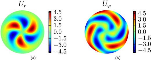
Equatorial slices of (a) the radial component u_r and (b) the azimuthal component u_φ of the velocity field for Benchmark 1. The velocity field is equatorially antisymmetric and thus the latitudinal component u_θ is zero in the equatorial plane.

Figure 2.

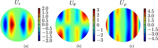
Meridional slices of the velocity field |$ {\bf u}$| for Benchmark 1: (a) radial component u_r, (b) latitudinal component u_θ and (c) azimuthal component u_φ. The slices are chosen such that they contain the maximal amplitude of the velocity field |$| {\bf u}|$|⁠.

Once the stable regime is reached, the solution exhibits a constant kinetic energy

\begin{eqnarray} E_{\rm k} = \frac{1}{2}\int _{V} { {\bf u}}^2 \mathrm{d}V \end{eqnarray}

(12)

providing an ideal diagnostic for the comparison among the different submissions (Fig. 3).

Figure 3.

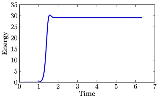
Typical time evolution of the kinetic energy E_k for Benchmark 1. After the initial transient, the kinetic energy reaches a constant value.

Furthermore, the whole solution is slowly drifting at a constant drift frequency. Similarly to what was done in B1, the velocity field of the solution can be described as

\begin{eqnarray} {\bf u} = {\bf u}(r,\theta ,\varphi -2\pi f_{\rm d} t), \end{eqnarray}

(13)

where f_d is the drift frequency in units of s⁻¹. The drift frequency f_d is related to the angular velocity or drift rate ω_d in units of rad s⁻¹ by

\begin{eqnarray} \omega _{\rm d} = {2 \pi }{f_{\rm d}}. \end{eqnarray}

(14)

With this choice of definition, due to the threefold spatial symmetry (see Fig. 1a), the drift frequency f_d represents the frequency at which a given flow pattern will pass through a fixed point in space. The whole solution pattern completes a full rotation at a frequency |$\tilde{f}_{\rm d} = f_{\rm d}/3$|⁠.

To compare the results of the six participants in Benchmark 1, the constant kinetic energy E_k and the drift frequency f_d of their solution were requested.

2.2 Benchmark 2: thermally driven dynamo

Benchmark 2 extends the first benchmark by incorporating the generation and evolution of magnetic fields. While still working within the frame of the Boussinesq approximation, the sphere is now filled with a conducting fluid with magnetic diffusivity η and magnetic permeability μ. It is still thermally forced through the presence of a homogeneous distribution of heat sources resulting in the basic state given by eq. (2). The system of equations is extended by the induction equation to describe the evolution of the magnetic field |$\bf B$|⁠. The equations are non-dimensionalized using the radius r_o as length scale, the magnetic diffusion time |$r_o^2/\eta$| as timescale, |$\beta r_o^2$| as the temperature scale and the magnetic field is rescaled by |$\sqrt{2\Omega \rho \mu \eta }$|⁠. The four required parameters are the Ekman number E

\begin{equation} E = \frac{\nu }{2\Omega r_o^2}, \end{equation}

(15)

the magnetic Rossby number (also referred to as the magnetic Ekman number) Ro

\begin{equation} Ro = \frac{E}{Pm} = \frac{\eta }{2\Omega r_o^2}, \end{equation}

(16)

the Roberts number q

\begin{equation} q = \frac{Pm}{Pr} = \frac{\kappa }{\eta }, \end{equation}

(17)

with κ the thermal diffusivity and the Rayleigh number Ra

\begin{equation} Ra = \frac{g\alpha \beta r_o^3}{2\Omega \kappa }, \end{equation}

(18)

with α the thermal expansion coefficient. To ease the conversion to different choices of non-dimensionalizations, the Prandtl number Pr

\begin{equation} Pr = \frac{\nu }{\kappa } = \frac{Pm}{q} = \frac{E}{q Ro}, \end{equation}

(19)

and the magnetic Prandtl number Pm

\begin{equation} Pm = \frac{\nu }{\eta } = \frac{E}{Ro}, \end{equation}

(20)

are also introduced. The motion of the conducting fluid is described by the non-dimensional Navier–Stokes equation and the incompressibility condition for the velocity field |$ {\bf u}$|

\begin{eqnarray} \left( Ro\partial _t - E\nabla ^2 \right) {\bf u} &= & Ro {\bf u}\wedge \left( \nabla \wedge {\bf u} \right) + \left( \nabla \wedge {\bf B} \right)\wedge {\bf B}\nonumber\\ && +\; q Ra T\! {\bf r} - {\skew 3\hat{ {\bf z}}}\wedge {\bf u} - \nabla \pi , \end{eqnarray}

(21)

\begin{eqnarray} \nabla \cdot {\bf u} = & 0. \end{eqnarray}

(22)

The magnetic induction equation and the solenoidal condition for the magnetic field |${\bf B}$| read as

\begin{eqnarray} \left( \partial _t - \nabla ^2 \right){\bf B} = & \nabla \wedge \left( {\bf u}\wedge {\bf B} \right), \end{eqnarray}

(23)

\begin{eqnarray} \nabla \cdot {\bf B} = 0, \end{eqnarray}

(24)

and finally the transport equation for the temperature T is given by

\begin{equation} \left(\partial _t - q\nabla ^2\right)T = S - {\bf u}\cdot \nabla T. \end{equation}

(25)

As for Benchmark 1, the outer boundary is maintained at fixed temperature and a stress-free mechanical boundary condition is imposed. Furthermore, the outer region is considered to be a perfect insulator.

The thermal dynamo solution for Benchmark 2 is obtained for an Ekman number E = 5 × 10⁻⁴, a magnetic Rossby number |$Ro = \frac{5}{7}\times 10^{-4}$|⁠, a Roberts number q = 7, a Rayleigh number Ra = 200 and a source term S = 3q = 21. In terms of the Prandtl numbers, the Benchmark 2 is obtained for a Prandtl number Pr = 1 and a magnetic Prandtl Pm = 7. This parameter regime is approximately two times supercritical and a magnetic field is generated and sustained by the system. Although the solution for Benchmark 2 can be obtained by starting from a small initial perturbation, the convergence to the final state is extremely slow and requires prohibitively high computational resources. Furthermore, the presence of several solution branches can not be excluded even if it was not seen during the computations. To reduce the computational load to a reasonable level, a special initial condition exhibiting a much faster convergence has been worked out.

The temperature field T should be initialized with the background conducting state with a small perturbation as a spherical harmonic of degree and order 3

\begin{eqnarray} T = \frac{1}{2}\left(1 - r^2\right) + \frac{\epsilon }{8}\sqrt{\frac{35}{\pi }}r^3\left(1-r^2\right)\left(\cos 3\varphi +\sin 3\varphi \right)\sin ^3\theta \nonumber\\ \end{eqnarray}

(26)

with ϵ = 10⁻⁵. The magnetic field should be initialized with a purely toroidal magnetic field given by

\begin{eqnarray} B_r = 0, \end{eqnarray}

(27)

\begin{eqnarray} B_{\theta } = -\frac{3}{2}r\left(-1+4r^2-6r^4+3r^6\right)\left(\cos {\varphi }+\sin {\varphi }\right), \end{eqnarray}

(28)

\begin{eqnarray} B_{\varphi } &= & -\frac{3}{4}r\left(-1 + r^2\right)\cos {\theta }\left[3r\left(2-5r^2+4r^4\right)\sin {\theta } \right.\nonumber \\ &&\left. +\; 2\left(1-3r^2+3r^4\right)\left(\cos {\varphi }-\sin {\varphi }\right)\right]. \end{eqnarray}

(29)

Finally, the velocity field should be initialized with a purely toroidal velocity given by

\begin{eqnarray} u_r = 0, \end{eqnarray}

(30)

\begin{eqnarray} u_{\theta } &= & -\frac{10 r^2}{7\sqrt{3}}\cos {\theta }\big [3\big (\!-\!147+343r^2-217r^4+29r^6\big )\cos {\varphi }\nonumber\\ && +\; 14\big (\!-\!9-125r^2+39r^4+27r^6\big )\sin {\varphi }\big ], \end{eqnarray}

(31)

\begin{eqnarray} u_{\varphi } &= & -\frac{5 r}{5544} \big \lbrace 7\big [(43\,700 - 58\,113r^2-15\,345r^4\nonumber\\ &&+\;1881r^6+20\,790r^8)\sin {\theta } \nonumber \\ &&+\; 1485r^2\left( -9 + 115r^2 - 167r^4+70r^6 \right)\sin {3\theta } \big ]\nonumber \\ &&+\; 528\sqrt{3} r\cos {2\theta }\big [14\left( -9-125r^2+39r^4+27r^6 \right)\cos {\varphi } \nonumber \\ && +\; 3\left( 147 - 343r^2 + 217r^4 - 29r^6 \right)\sin {\varphi } \big ] \big \rbrace . \end{eqnarray}

(32)

For simulations using spherical harmonics and a toroidal/poloidal decomposition, the expression of the initial conditions can be written in a simpler form. Assuming that the magnetic field is decomposed as |${\bf B} = {\bf \nabla }\wedge {\mathcal {T} {\bf r}} + {\bf \nabla }\wedge {\bf \nabla }\wedge {\mathcal {P} {\bf r}}$|⁠, the initial field is given by the two scalars

\begin{eqnarray} \mathcal {T} &\!=\! & r\left[\left(\frac{3}{4} \!-\! 3r^2 \!+\! \frac{9}{2}r^4 \!-\! \frac{9}{4}r^6\right) \!+\! \left(\frac{3}{4} \!-\! 3r^2 \!+\! \frac{9}{2}r^4 \!-\! \frac{9}{4}r^6\right)\imath \right]\mathcal {Y}_{1}^{1}\nonumber \\ &&+\; r^2\left(\frac{3}{2} - \frac{21}{4}r^2 + \frac{27}{4}r^4 - 3r^6\right)\mathcal {Y}_{2}^{0} + c.c., \end{eqnarray}

(33)

\begin{eqnarray} \mathcal {P} = 0, \end{eqnarray}

(34)

where c.c. stands for the complex conjugate without the m = 0 modes and |$\mathcal {Y}_{l}^{m}$| are Schmidt normalized complex spherical harmonics. Similarly assuming that the velocity field is decomposed as |$ {\bf u} = {\bf \nabla }\wedge {T {\bf r}} + {\bf \nabla }\wedge {\bf \nabla }\wedge {P {\bf r}}$|⁠, the initial condition is given by

\begin{eqnarray} T &= & r^2\bigg[\left(30 + \frac{1250}{3}r^2 - 130r^4 - 90r^6\right)\nonumber\\ &&+ \left(105 - 245r^2 + 155r^4 - \frac{145}{7}r^6\right)\imath \bigg]\mathcal {Y}_{2}^{1}\nonumber \\ && +\;r\left(-\frac{54\,625}{198} + 350r^2 + \frac{625}{2}r^4 - 325r^6\right)\mathcal {Y}_{1}^{0}\nonumber\\ &&+\; r^3\left(45 - 575r^2 + 835r^4 - 350r^6\right)\mathcal {Y}_{3}^{0} +\; c.c., \end{eqnarray}

(35)

\begin{eqnarray} P = & 0. \end{eqnarray}

(36)

Details of the definition and the normalization of the spherical harmonics |$\mathcal {Y}_{l}^{m}$| are given in Appendix A.

The structure of the solution to Benchmark 2 is much more complicated than for Benchmark 1 and no longer exhibits a simple symmetry. Nevertheless, after the initial transient the system settles into a regime with periodic kinetic and magnetic energies. The amplitude and frequency of these oscillations provide a good diagnostic for Benchmark 2 (Fig. 4).

Figure 4.

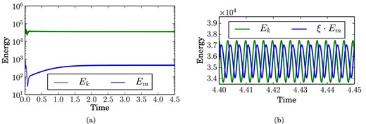
Kinetic energy E_k and magnetic energy E_m for Benchmark 2. (a) Typical time evolution of E_k and E_m. After the initial transient, both energies settle into a periodic oscillation. (b) Detailed view of the oscillations in E_k and E_m. The magnetic energy has been rescaled by |$\xi = \frac{C_{\rm k}}{C_{\rm m}} \approx 39$| (see eqs 37 and 40) to show the phase shift between E_k and E_m.

To illustrate the structure of the velocity field, a few equatorial slices are shown in Fig. 5. The time-dependent features of the solutions can be seen in the Hammer projection snapshots of the flow close to the outer boundary (Fig. 6) and the Hammer projections of the radial component of the magnetic field at the outer boundary (Fig. 7). The two comma shaped flux patches of opposite sign emerge periodically. The lower part moves eastwards while rising to higher latitudes until they vanish. Fig 7 shows snapshots over approximately two periods.

Figure 5.

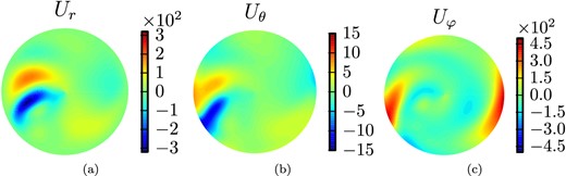
Equatorial slices of the velocity field |$ {\bf u}$| at t = 4.43241 for Benchmark 2: (a) radial component u_r, (b) latitudinal component u_θ and (c) azimuthal component u_φ.

Figure 6.

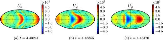
Hammer projections of three snapshots of the azimuthal velocity component u_φ at the outer boundary (r = r_o) for Benchmark 2.

Figure 7.

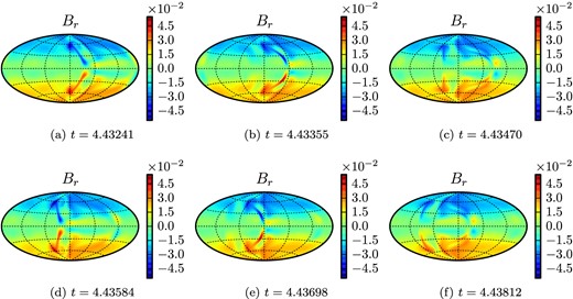
Hammer projections of six snapshots, spanning approximatively two periods, of the radial magnetic field B_r at the outer boundary r = r_o for Benchmark 2.

The solution to Benchmark 2 will solely be characterized by the computed kinetic and magnetic energies. Their periodic behaviour allows us to define several diagnostic quantities used to compare the solutions from different simulations. The kinetic energy is decomposed into a constant component C_k, the amplitude of the leading oscillating term A_k, the frequency of this oscillation f_k and a phase shift ζ_k. Using these definitions,the kinetic energy E_k is written as

\begin{eqnarray} E_{\rm k} = \frac{1}{2}\int _{V} {\bf u}^2 \mathrm{d}V = C_{\rm k} + A_{\rm k} \cos (2\pi f_{\rm k} t + \zeta _{\rm k}) + \cdots \end{eqnarray}

(37)

Furthermore, decomposing the velocity into its equatorially symmetric [labelled as (s)] and equatorially antisymmetric part [labelled as (a)], the velocity field was found to be purely equatorially symmetric

\begin{eqnarray} E_{\rm k}^{(s)} = E_{\rm k}, \end{eqnarray}

(38)

\begin{eqnarray} E_{\rm k}^{(a)} = 0. \end{eqnarray}

(39)

Using the same decomposition, the magnetic energy E_m can be written as

\begin{eqnarray} E_{\rm m} =\frac{1}{2 Ro}\int _{V} {{\bf B}}^2 \mathrm{d}V = C_{\rm m} + A_{\rm m} \cos (2\pi f_{\rm m} t + \zeta _{\rm m}) + \cdots \end{eqnarray}

(40)

Decomposing the magnetic field into its equatorially symmetric and antisymmetric parts, the magnetic field is found to be purely equatorially antisymmetric

\begin{eqnarray} E_{\rm m}^{(s)} = 0, \end{eqnarray}

(41)

\begin{eqnarray} E_{\rm m}^{(a)} = E_{\rm m}. \end{eqnarray}

(42)

It was found and confirmed by all participants that the oscillations in the magnetic energy and kinetic energy have the same frequency. In addition, as can be seen in Fig. 4(b), there is a phase shift between the magnetic and kinetic energy. This relative phase shift (ζ_k − ζ_m) is found to have value 1.91rad but is not included in the benchmark. The six constants C_k, A_k, f_k, C_m, A_m and f_m defined above are the diagnostic values that were requested from all submissions to Benchmark 2.

The computation of decompositions 37 and 40 requires some further explanations as several different approaches are possible. The first one involves computing the Fourier series. To reduce the spectral leakage, a flat top window (Oliphant 2007) is applied on the time-series. The amplitude of the different modes can then easily be extracted as shown in Fig. 8(a). Conversely, to compute an accurate frequency, a Kaiser window (Kaiser & Kuo 1966) with parameter β = 14 is applied to the time-series. The peaks in the spectrum are then well approximated with a parabolic fit allowing for interpolation between the available frequencies. The peak for the main oscillation is shown in Fig. 8(b). The frequencies can also be computed by counting the zero crossings. Both approaches provide the frequency within a relative error of 10⁻⁴ per cent. There is a simpler approach to obtain the requested data without using a Fourier transform. Assuming |$E_i^{\rm min}$|⁠, |$E_i^{\rm max}$| are the minimum and maximum of the time-series for the energy, the constant component is approximatively given by

\begin{eqnarray} C_i \approx \frac{E_i^{\rm min} + E_i^{\rm max}}{2}, \end{eqnarray}

(43)

and the amplitude of the main oscillation is approximatively given by

\begin{eqnarray} A_i \approx \frac{E_i^{\rm max} - E_i^{\rm min}}{2}. \end{eqnarray}

(44)

These relations are not exact because the time-series do also include higher frequencies as shown in Fig. 8(a). Using the Fourier series, it is possible to bound the relative errors generated by the simplified approach. By including the second peak with a frequency of 2f_i and accounting for the phase shift, a comparison with the approximations 43 and 44 provides the relative errors |$\epsilon _{C_{\rm k}}$| and |$\epsilon _{A_{\rm k}}$| on C_k and A_k for the kinetic energy

\begin{eqnarray} \epsilon _{C_{\rm k}} & = & 3\times 10^{-2} \ \mathrm{per\ cent}, \end{eqnarray}

(45)

\begin{eqnarray} \epsilon _{A_{\rm k}} & = & 5\times 10^{-2} \ \mathrm{per\ cent}. \end{eqnarray}

(46)

The same analysis on the magnetic energy provides the relative errors |$\epsilon _{C_{\rm m}}$| and |$\epsilon _{A_{\rm m}}$| on C_m and A_m

\begin{eqnarray} \epsilon _{C_{\rm m}} & = & 0.4 \ \mathrm{per\ cent}, \end{eqnarray}

(47)

\begin{eqnarray} \epsilon _{A_{\rm m}} & = & 0.6 \ \mathrm{per\ cent}. \end{eqnarray}

(48)

These relative errors have been obtained by assuming that |$E_i^{\rm min}$| and |$E_i^{\rm max}$| are exact. An accurate value for the minimum and maximum requires a time-series sampled at a high frequency but it does in principle only require one cycle. On the other hand, an accurate Fourier series will require a long time-series. The errors made by using this simplified approach depend strongly on the relative magnitude of the higher frequencies. For the kinetic energy, the second oscillation with a frequency of 2f_k has an approximatively 63 times smaller amplitude which leads to the rather small errors given in eqs (45) and (46). On the other hand, the second oscillation in the magnetic energy is only approximatively 10 times smaller leading to the larger errors given in eqs (47) and (48). In both cases, the third oscillation with a frequency 3f can be neglected as it is more than 20 times smaller than the second oscillation.

Figure 8.

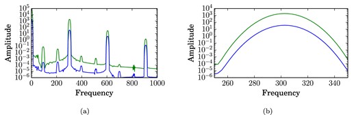
(a) Frequency spectrum of the kinetic energy E_k and magnetic energy E_m for Benchmark 2 after a flat top window has been applied on the time-series. (b) Details of the peak of the main amplitude of the kinetic and magnetic energies after a Kaiser window with parameter β = 14 has been applied to the time-series. Note the use of a logarithmic scale for the ordinate, meaning that the frequency localization is extremely good. Both spectra have been obtained on a time-series over approximatively 0.35 diffusion times at a sampling rate of 1.75 × 10⁵ obtained by (MJ) at N = 31 and L = M = 63 (see Section 3 for details).

2.3 Benchmark 3: boundary forced rotating bubble

Benchmark 3 is again a purely hydrodynamic problem. It provides a simple test problem for boundary driven flows in a whole sphere as they might, for example, arise in precession or libration problems. The proposed system describes the motion of an incompressible fluid inside a spherical bubble rising in a rotating fluid. It is an important addition to the first two cases as it replaces the internal thermal forcing by a mechanical forcing due to an imposed tangential flow over the boundary. The bubble is assumed to be of unit radius r_o = 1 and is described by the Navier–Stokes equation and incompressibility condition

\begin{eqnarray} \partial _t {\bf u} + {\bf u}\cdot \nabla {\bf u} + 2\Omega {\skew 3\hat {\bf z}}\wedge {\bf u} = & - \nabla p + \nu \nabla ^2 {\bf u}, \end{eqnarray}

(49)

\begin{eqnarray} \nabla \cdot {\bf u} = & 0 \end{eqnarray}

(50)

with ν the viscosity of the fluid and Ω the rotation rate of the bubble. The rotation axis is parallel to |${\skew 3\hat{ {\bf z}}}$|⁠. The tangential flow over the boundary imposes a non-homogeneous boundary condition on the fluid at the surface of the bubble

\begin{eqnarray} u_\theta = -u_0 \cos \theta \cos \phi , \end{eqnarray}

(51)

\begin{eqnarray} u_\phi = u_0 \sin \phi , \end{eqnarray}

(52)

which is the gradient of a pure l = 1, m = 1 spherical harmonic |$\mathcal {Y}_{1}^{1}(\theta ,\phi )$|⁠.

The solution to Benchmark 3 is obtained for a boundary velocity |$u_0 = \scriptstyle\sqrt{\frac{3}{2\pi }}$|⁠, a viscosity ν = 10⁻² and a rotation rate Ω = 10. It does not require any particular initial condition and can be started with a zero initial velocity field.

The flow converges quickly to a stationary solution with a dominant m = 1 component. Interestingly, the solution contains an important and non-trivial flow through the centre of the bubble. As such, it provides a good diagnostic for this numerically challenging region. To illustrate the flow of the solution, the velocity field components in the x − z and y − z planes are shown in Fig. 9. The velocity field in the x − y plane, which is orthogonal to the rotation axis (i.e. the equatorial plane) is shown in Fig. 10.

Figure 9.

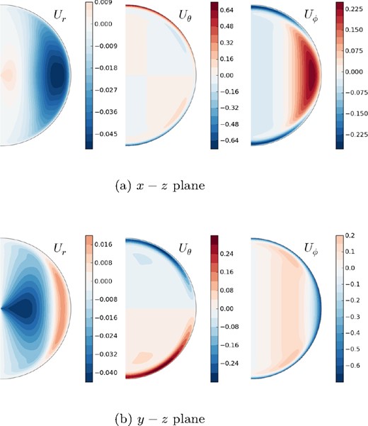
In the top row, velocity field in the x–z plane (ϕ = 0) and in the bottom row, velocity field in the y–z plane (ϕ = π/2) for Benchmark 3.

Figure 10.

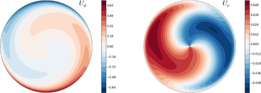
Velocity field in the x–y (equatorial) plane for Benchmark 3.

The solution to Benchmark 3 was characterized by five diagnostic values. The first diagnostic is the constant kinetic energy

\begin{eqnarray} E_{\rm k} = \frac{1}{2}\int _{V} { {\bf u}}^2 \mathrm{d}V \end{eqnarray}

(53)

reached after the initial transient. When available, the energy in the spherical harmonic orders m = 0, m = 1 and m = 2 have also been collected. Secondly, the |${\skew 3\hat{ {\bf z}}}$| component of the angular momentum L_z is reported. The three components of the velocity field |$ {\bf u}$| at the centre of the bubble provide that last diagnostic data.

3 CONTRIBUTING NUMERICAL CODES

There was a total of nine contributors to the benchmark but each did not necessarily provide results for all three cases. A short description of the algorithm used by each simulation is provided below. Further references are given for a more detailed description.

Marti and Jackson (MJ): Spectral simulation using spherical harmonics for the angular component and polynomials developed by Worland (2004) and Livermore et al. (2007) in radius (see Marti 2012). The Worland polynomials satisfy exactly the parity and regularity conditions required at the origin of the spherical coordinate system. Specifically, the radial basis used is of the form |$r^l P_n^{(-1/2,l-1/2)}(2r^2-1)$| for a given harmonic degree l, with |$P^{(\alpha ,\beta )}_n(x)$| the Jacobi polynomials. The incompressibility condition is guaranteed by the use of a toroidal/poloidal decomposition of the vector fields. A second-order predictor–corrector scheme is used for the time integration. No specific treatment is required to conserve angular momentum.

Hollerbach (H): An adaptation of the previous spherical shell code described by Hollerbach (2000), based on spherical harmonics and a toroidal/poloidal decomposition of the vector fields. Instead of expanding in the full set of Chebyshev polynomials in radius, regularity and parity conditions at the origin are now accommodated by expanding as r · T_{2k − 1}(r) for odd harmonic degrees and r² · T_{2k − 1}(r) for even harmonic degrees for the toroidal/poloidal scalars. The temperature is similarly expanded as T_{2k − 2}(r) for degree l = 0, r · T_{2k − 2}(r) for odd degrees, and r² · T_{2k − 2}(r) for even degrees. Angular momentum conservation is explicitly imposed by a modified stress-free boundary condition.

Aubert (A): Spectral simulation using the code PARODY-JA, which uses spherical harmonics for the angular component and a second-order finite differences in radius (see Dormy et al.1998; Aubert et al.2008). The time marching is done with a semi-implicit Crank–Nicolson/Adams–Bashforth scheme. The radial mesh includes a gridpoint exactly at the centre of the sphere. Spectral toroidal and poloidal components of order l behave like r ^l at the centre. Angular momentum conservation is achieved by correcting for solid-body rotation at each time step.

Schaeffer (S): Spectral simulation using spherical harmonics for the angular component and second-order finite differences in radius (Monteux et al.2012). The numerical instability near the origin is overcome by truncating the spherical harmonic expansion at ℓ_tr(r) before computing the spatial fields that enter the non-linear terms. Specifically, the truncation is |$\ell _{\rm tr}(r) = 1 + (\ell _{\rm max}-1) \left( \frac{r}{r_o} \right)^\alpha$|⁠, where α = 0.5 gives good results, and also saves some computation time. The time stepping uses a semi-implicit Crank–Nicolson scheme for the diffusive terms, while the non-linear terms can be handled either by an Adams–Bashforth or a predictor–corrector scheme (both second-order in time). The SHTns library (Schaeffer 2013) is used for efficient spherical harmonic transforms. Angular momentum conservation is achieved by adjusting the solid-body rotation component at each time step.

Takehiro, Sasaki and Hayashi (TSH): Spectral simulation using spherical harmonics for the angular components and the polynomials developed by Matsushima & Marcus (1995) and Boyd (2001) in radius (see Sasaki et al.2012). The radial basis functions satisfy exactly the parity and regularity conditions at the origin of the spherical coordinate system. Specifically, the used radial basis is of the form |$r^l P_n^{(\alpha ,\beta )}(2r^2-1)$| for a given harmonic degree l, with P_n(x) the Jacobi polynomials. The incompressibility condition is guaranteed by the use of a toroidal/poloidal decomposition of the vector fields. The time integration is performed with the Crank–Nicolson scheme for the diffusive terms and a second-order Adams–Bashforth scheme for the other terms. No specific treatment is required to conserve angular momentum.

Simitev and Busse (SB): Pseudospectral numerical code using spherical harmonics expansion in the angular variables and Chebyshev polynomials in radius. Time stepping is implemented by a combination of the implicit Crank–Nicolson scheme for the diffusion terms and the explicit Adams–Bashforth scheme for the Coriolis and the non-linear terms; both schemes are second-order accurate. Early versions of the code are described in Tilgner & Busse (1997) and Tilgner (1999). The code has been extensively modified and used for a number of years (Simitev & Busse 2005, 2009, 2012; Busse & Simitev 2006, 2008). This is a spherical shell code and no special effort was made to convert it to the full sphere geometry. Instead, the full sphere is approximated by placing a tiny inner core with radius ratio r_i/r_o = 0.01 at the centre of the shell. Angular momentum conservation is achieved by correcting for rigid-body rotation if required.

Cébron (C): Finite elements method simulation using the standard Lagrange element P2–P3, which is quadratic for the pressure field and cubic for the velocity field, and a Galerkin Least-Squares (GLS) stabilization method (Hauke & Hughes 1994). The (unstructured) mesh is made of prisms in the boundary layer and tetrahedrons in the bulk. The incompressibility is imposed using a penalty method. The time stepping uses the Implicit Differential-Algebraic solver (IDA solver), based on variable-coefficient Backward Differencing Formulae (e.g. Hindmarsh et al.2005). The integration method in IDA is variable-order, the order ranging between 1 and 5. At each time step, the system is solved with the sparse direct linear solver PARDISO (www.pardiso-project.org) or a multigrid GMRES iterative solver. This is all implemented via the commercial code COMSOL Multiphysics^®.

Nore, Luddens and Guermond (NLG): Hybrid Fourier and finite element method using a Fourier decomposition in the azimuthal direction and the standard Lagrange elements P1–P2 in the meridian section (with P1 for the pressure and P2 for the velocity field). The meridian mesh is made of quadratic triangles. The velocity and pressure are decoupled by using the rotational pressure-correction method. The time stepping uses the second-order Backward Difference Formula (BDF2). The non-linear terms are made explicit and approximated using second-order extrapolation in time. The code is parallelized in Fourier space and in meridian sections [domain decomposition with METIS (Karypis & Kumar 2009)] using MPI and PETSC (Portable, Extensible Toolkit for Scientific Computation; Balay et al.1997, 2012a,b). This is implemented in the code SFEMaNS (for Spectral/Finite Element method for Maxwell and Navier–Stokes equations; Guermond et al.2007, 2009, 2011).

Vantieghem (V): Unstructured finite-volume simulation (see Vantieghem 2011) using a grid of tetrahedral elements with smaller elements close to the wall. The spatial discretization is based on a centred-difference-like stencil that is second-order accurate for regular tetrahedra. Time stepping is based on a canonical fractional-step method (Kim & Moin 1985), and the equations are integrated in time with a fourth order Runge–Kutta method. A BiCGstab(2) algorithm is used to solve the pressure Poisson equation. The reported Fourier components are obtained by an a posteriori interpolation of the results on a regular grid in terms of spherical coordinates (N_r = 36, N_θ = N_φ = 18), which is subject to considerable additional numerical (interpolation) errors.

4 RESULTS

There is quite an important diversity in the type of simulations that took part in these benchmarks. All the diagnostics that have been considered for these benchmarks should be straightforward to obtain whenever the simulation code is based on some spectral expansion or on a local method. On the other hand, a direct comparison of the resolution used is a more subtle problem. The comparison will be done by comparing solutions based on the number of degrees of freedom present at the time stepping level. For local methods, the resolution R is computed as |$R = N_{\rm grid}^{1/3}$| where N_grid is the number of gridpoints and for spherical harmonic–based codes |$R = \left\lbrace N_r\cdot \left[L_{\rm max}(2M_{\rm max}+1)- M_{\rm max}^2 + M_{\rm max} + 1\right]\right\rbrace ^{1/3}$|⁠. The same approach was used in B1.

4.1 Benchmark 1

There were six participants in Benchmark 1 and all of them used a spherical harmonics–based simulation. They agree qualitatively quite well and no important discrepancies were found. The details of all the solutions obtained by the participants is given in Table 1. At the quantitative level, a few interesting observations can be made. The results for the total kinetic energy are summarized in Fig. 11(a). The five codes (MJ), (H), (TSH), (S), (A) do all eventually converge to the same solution within 5 × 10⁻² per cent. While using a completely different radial expansion, (MJ) and (H) even converge very rapidly within 5 × 10⁻⁴ per cent. The last code (SB) working in a spherical shell rather than a sphere comes within 0.4 per cent. Note that the results obtained with a very high radial resolution (1600 gridpoints) by (A) matches very closely to the solutions from the fully spectral codes. The other finite differences–based code (S) shows a clear convergence towards the same solution and would most likely have reached it at a higher resolution.

Figure 11.

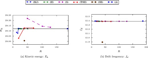
Summary of the solutions of the participants of Benchmark 1. (a) Constant kinetic energy E_k, as defined in eq. (12), reached after the initial transient. (b) Drift frequency f_d, defined in Section 2, of the threefold symmetric structure of the solution (see Fig. 1). The black horizontal line is the standard value given in Table 2. The error corridor for the standard values is represented by a greyed out area, but as the errors are very small it is only barely visible. The labels used for the different codes are defined in Section 3.

Table 1.

Contributions to Benchmark 1. The labels used for the different codes are defined in Section 3. The values are shown with the number of significant digits provided by the authors. As all these codes are based on a spherical harmonics expansion for the angular component, the resolution is given as the radial resolution N, the highest harmonic degree L and the highest harmonic order M.

Code	Ek	fd	N	L	M
(MJ)	29.08502	12.38841	8	15	15
(MJ)	29.07661	12.38860	8	23	23
(MJ)	29.12178	12.38604	12	23	23
(MJ)	29.12064	12.38619	16	23	23
(MJ)	29.12064	12.38619	16	31	31
(MJ)	29.12068	12.38619	23	47	47
(MJ)	29.12068	12.38619	31	63	63
(H)	29.11784	12.3862	12	23	23
(H)	29.12054	12.3862	16	31	31
(H)	29.12053	12.3862	23	31	31
(H)	29.12053	12.3862	23	47	47
(H)	29.12053	12.3862	31	63	63
(S)	29.219	12.388	120	31	31
(S)	29.1446	12.387	250	63	63
(S)	29.13501	12.38648	320	85	85
(TSH)	29.03074	12.3878	16	21	21
(TSH)	29.12878	12.3863	32	42	42
(TSH)	29.12878	12.3863	48	85	85
(SB)	29.00617	11.89445	33	42	42
(A)	29.12062	12.3931	1600	63	63

The picture is very similar for the drift frequency (Fig. 11b). The codes (MJ), (H) and (TSH) agree within 6 × 10⁻⁴ per cent , the solution by (S) is within 2 × 10⁻³ per cent and the solution by (A) is within 6 × 10⁻² per cent. Finally, the solution by (SB) is within 4 per cent.

A standard value for the kinetic energy and drift frequency for Benchmark 1 is derived from the three simulations showing the best convergence to a common result. The values as well as a short summary of the problem definition are given in Table 2. The very high convergence to a common solution allow to provide these with roughly six significant digits.

Table 2.

Summary table and standard values obtained for Benchmark 1. The Ekman number E, the Prandtl number Pr and the modified Rayleigh number Ra as well as the governing equation for the velocity |$ {\bf u}$| and the temperature T are given in Section 2. The kinetic energy E_k is defined in eq. (12) and the drift frequency by eq. (13).

Benchmark 1: Thermal convection
Parameters
E	Pr	Ra
3 × 10−4	1	95
Boundary conditions
|$ {\bf u}$|⁠:	stress-free
T:	fixed temperature
	homogeneous heat sources
Requested values
Ek	29.1206	±1 × 10−4
fd	12.3862	±1 × 10−4

4.2 Benchmark 2

All the groups participating in Benchmark 1 also participated in Benchmark 2, except for (A). There are thus again only solutions from spherical harmonics–based simulations. The overall picture is very similar to Benchmark 1. The fully spectral simulations converge very rapidly to their final solution and which are in most cases very close to each other. The finite differences simulation, while requiring higher radial resolution, eventually reaches a similar solution. As was already observed in Benchmark 1, the simulation by (SB) which approximates the whole sphere as a shell with a tiny inner core, shows the largest discrepancy. The details of all the solutions to Benchmark 2 are given in Table 3.

Table 3.

Spectral method contributions to Benchmark 2. The labels used for the different codes are defined in Section 3. The values are shown with the number of significant digits provided by the authors. The decomposition of the kinetic energy E_k into C_k, A_k and f_k is defined in eq. (37) and the equivalent decomposition of the magnetic energy E_m into C_m, A_m and f_m is defined in eq. (40). As all these codes are based on a spherical harmonic expansion for the angular component, the resolution is given as the radial resolution N, the highest harmonic degree L and the highest harmonic order M.

Code	Ck	Ak	fk	Cm	Am	fm	N	L	M
(MJ)	35 141.84	1836.287	302.2623	1153.695	51.77003	302.2623	12	23	23
(MJ)	35 548.95	1881.661	302.6947	922.3073	38.54002	302.6947	16	31	31
(MJ)	35 542.15	1880.460	302.6858	924.5757	38.48190	302.6858	23	31	31
(MJ)	35 551.33	1880.055	302.7018	908.9870	37.47705	302.7018	23	47	47
(MJ)	35 550.93	1879.837	302.7015	908.8059	37.45069	302.7015	31	63	63
(H)	35 378	1855	302.48	1043.77	46.16	302.48	12	23	23
(H)	35 588	1885	302.71	904.30	37.61	302.71	16	31	31
(H)	35 540	1881	302.66	925.64	38.50	302.66	23	31	31
(H)	35 551	1880	302.67	909.67	37.48	302.67	23	47	47
(H)	35 550	1880	302.67	909.46	37.47	302.67	31	63	63
(S)	35 544	1878.1	302.2	951.59	41.33	302.2	120	31	31
(S)	35 568	1881.0	302.65	908.69	37.951	302.65	250	63	63
(S)	35 552	1880.1	302.11	910.75	38.064	302.11	320	85	85
(TSH)	35 619.63	1887.200	303.0303	881.6272	36.97913	303.0303	32	42	42
(TSH)	35 564.30	1872.702	303.0303	905.8444	37.60794	303.0303	48	85	85
(SB)	35 951.5	1843.38	304.308	1046.12	38.08	304.308	41	96	96

The solutions obtained by the different simulations are summarized in Figs 12(a)–(e). For the constant part of the kinetic (C_k) and magnetic (C_m) energies, excluding the solution by (SB), all results lie within 2 × 10⁻² and 0.3 per cent, respectively. A good convergence to a common solution was also observed for the amplitude of the oscillations in the kinetic energy. The solutions provided by (MJ), (H) and (S) lie within 7 × 10⁻³ per cent. The solution of (TSH) does not seem to converge to exactly the same value but remains within 0.4 per cent of the three other values. The convergence is not as good for the amplitude in the oscillation of the magnetic energy. All the results lie within 1 per cent. The solution by (MJ), (H) and (TSH) seem to show the clearest convergence trend and their solutions lie within 0.2 per cent. Finally, the frequency of the oscillations of the kinetic and magnetic energies have been compared. All groups reported the same frequency f for both energies. The summary of the solutions for the frequency is shown in Fig. 12(e). The results for (MJ), (H), (TSH) and (S) lie within 0.3 per cent while (SB) is a little bit further away with 0.6 per cent.

Figure 12.

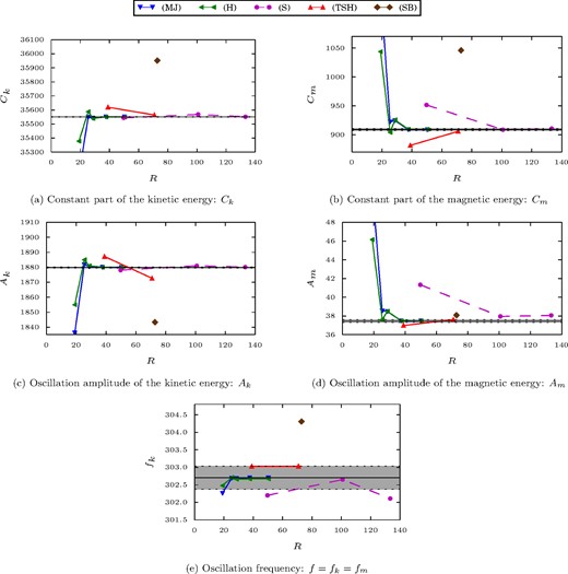
Summary of the solutions of the participants to Benchmark 2. The decomposition of the kinetic energy E_k into a constant part C_k, the amplitude of the main oscillation A_k and its frequency f_k is defined in eq. (37). The equivalent decomposition for the magnetic energy E_m, defining the three constants C_m, A_m and f_m is given in eq. (40). The black horizontal line is the standard value given in Table 4. The error corridor for the standard values, defined such that the three most converged solutions are included, is represented by a greyed out area. The labels used for the different codes are defined in Section 3.

While the spread in the solutions is clearly more important for Benchmark 2, the general situation is very similar to Benchmark 1. The solutions by (MJ) and (H) do nearly overlap for all five diagnostic values and do exhibit a very fast convergence. As was explained in Section 3, the extraction of the different components of the energies requires some post-processing. The choice of methodology by each author, for example, to extract the oscillation amplitude, might explain a part of the somewhat larger discrepancies compared to Benchmark 1. The standard values given in Table 4 are obtained by taking the average of the highest resolution by (MJ) and (H). The error bars are chosen such that at least one additional solution is included in the error corridor. This choice is based on the fast convergence of both codes to essentially the same value for all the requested data.

Table 4.

Summary table and standard values obtained for Benchmark 2. The Ekman number E, the magnetic Rossby number Ro, the Roberts number q and the modified Rayleigh number Ra, as well as the governing equations for the velocity |$ {\bf u}$|⁠, the magnetic field |${\bf B}$| and the temperature T are given in Section 2. The decomposition of the kinetic energy E_k into constant and oscillating components is defined in eq. (37) and the decomposition of the magnetic energy is defined in eq. (40).

Benchmark 2: Thermally driven dynamo
Parameters
E	Ro	q	Ra
5 × 10−4	5/7 × 10−4	7	200
Boundary conditions
|$ {\bf u}$|⁠:	stress-free
|${\bf B}$|⁠:	insulating
T:	fixed temperature
	homogeneous heat sources
Requested values
Kinetic energy Ek
	Ck	35 550.5	±1.5
	Ak	1879.84	±0.26
Magnetic energy Em
	Cm	909.133	±1.62
	Am	37.4603	±0.1476
Frequency f = fk = fm		302.701	±0.33
Additional characteristic
Phase shift	|ζk − ζm|	1.91rad

While it was not part of the actual benchmark, the phase shift between the kinetic and magnetic energy (see Fig. 4b) is also reported in Table 4 to provide a more complete characterization of the solution. The reported value has been computed by (MJ) from time-series of the kinetic and magnetic energy at the highest reported resolution (N = 31, L = M = 63). The phase shift has been extracted from the Fourier series shown in Fig. 8.

4.3 Benchmark 3

Benchmark 3 had the highest number of participants with eight codes taking part. It is also the only case where results from local methods are available. The computation for Benchmark 3 does not require a very high horizontal resolution. For example, spherical harmonics–based codes exhibit a very good convergence at resolutions as low as L_max = 30 and M_max = 10. However, it is more demanding in the radial direction. The centre requires a sufficiently high resolution to describe flow crossing it properly as well as the moving outer boundary which is forcing the system.

The solutions obtained by the different groups are summarized in Figs 13(a)–(e). Note that some of the solutions obtained by spherical harmonics–based codes have been obtained with a reduced longitudinal resolution while a triangular truncation was used for Benchmarks 1 and 2. The details for each solution are given in Table 5 for the spectral methods and in Table 6 for the local methods. A good convergence of the kinetic energy E_k is observed. Surprisingly, it is the solution by (TSH) which shows the largest discrepancy (0.4 per cent) while all the other solutions agree within 0.1 per cent at least. (MJ), (H), (S), (C) and (NLG) show the clearest convergence with solutions within 8 × 10⁻³ per cent. The values obtained for the vertical component of the angular momentum show the largest discrepancies among the diagnostics for Benchmark 3. The solutions by (H), (S), (C), (NLG), (V) seem to converge to the same value within 7 × 10⁻² per cent. While a very high agreement was achieved for the kinetic energy solutions, simulations by (MJ), (TSH) and (A) seem to converge to a lower value of L_z but still within 0.4 per cent. The last two diagnostic values involve the evaluation of the velocity field at the centre of the spherical domain. While all simulations lie within 0.15 per cent for the velocity along the y-axis, the velocity along the x-axis shows a larger discrepancy with values within 0.3 per cent.

Figure 13.

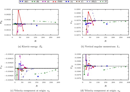
Summary of the solutions of the participants to Benchmark 3. The vertical velocity component u_z is not shown as it was consistently shown to be zero. The black horizontal line is the standard value given in Table 7. The error corridor for the standard values is represented by a greyed out area. Except for (c) which has larger errors, the error corridor is mostly hidden by the black line. The labels used for the different codes are defined in Section 3.

Table 5.

Spectral method contributions to Benchmark 3. The labels used for the different codes are defined in Section 3. The values are shown with the number of significant digits provided by the authors. As all these codes are based on a spherical harmonics expansion for the angular component, the resolution is given as the radial resolution N, the highest harmonic degree L and the highest harmonic order M.

Code	Ek	Ek, m = 0	Ek, m = 1	Ek, m = 2	Lz	Ux	Uy	N	L	M
(MJ)	6.18485e−2	4.35430e−4	6.12948e−2	1.17244e−4	2.78499e−2	−1.06714e−2	4.00811e−2	12	23	23
(MJ)	6.18338e−2	4.31265e−4	6.12841e−2	1.17319e−4	2.76877e−2	−8.91803e−3	3.86386e−2	16	23	23
(MJ)	6.18338e−2	4.31265e−4	6.12841e−2	1.17319e−4	2.76877e−2	−8.91803e−3	3.86386e−2	16	31	31
(MJ)	6.18291e−2	4.32506e−4	6.12783e−2	1.17195e−4	2.77151e−2	−8.21402e−3	3.83418e−2	23	31	31
(MJ)	6.18291e−2	4.32506e−4	6.12783e−2	1.17195e−4	2.77151e−2	−8.21402e−3	3.83418e−2	23	47	47
(MJ)	6.18286e−2	4.32813e−4	6.12776e−2	1.17118e−4	2.77204e−2	−8.27886e−3	3.83230e−2	31	47	47
(MJ)	6.18286e−2	4.32813e−4	6.12776e−2	1.17118e−4	2.77204e−2	−8.27885e−3	3.83230e−2	31	63	63
(H)	6.1832e−2	4.3521e−4	6.1278e−2	1.1762e−4	2.7783e−2	−1.0066e−2	3.7817e−2	12	12	4
(H)	6.1831e−2	4.3515e−4	6.1277e−2	1.1754e−4	2.7796e−2	−8.3410e−3	3.8318e−2	15	15	5
(H)	6.1831e−2	4.3514e−4	6.1277e−2	1.1754e−4	2.7796e−2	−8.2654e−3	3.8307e−2	18	18	6
(H)	6.1831e−2	4.3514e−4	6.1277e−2	1.1754e−4	2.7796e−2	−8.2644e−3	3.8307e−2	21	21	7
(H)	6.1831e−2	4.3514e−4	6.1277e−2	1.1754e−4	2.7796e−2	−8.2644e−3	3.8307e−2	24	24	8
(S)	6.15237e−2	4.25401e−4	6.09814e−2	1.15913e−4	2.748153e−2	−8.121293e−3	3.778225e−2	150	20	7
(S)	6.17682e−2	4.33033e−4	6.12169e−2	1.17198e−4	2.772647e−2	−8.230440e−3	3.820168e−2	300	20	7
(S)	6.17537e−2	4.32675e−4	6.12028e−2	1.17133e−4	2.771565e−2	−8.226658e−3	3.817840e−2	300	31	10
(S)	6.18047e−2	4.34295e−4	6.1252e−2	1.17400e−4	2.776804e−2	−8.251015e−3	3.826415e−2	500	31	10
(S)	6.18239e−2	4.34907e−4	6.12705e−2	1.17501e−4	2.778725e−2	−8.262105e−3	3.829847e−2	1000	31	10
(TSH)	5.98943e−2	3.63627e−4	5.94187e−2	1.10888e−4	2.53084e−2	−3.29031e−2	1.22471e−1	12	10	10
(TSH)	6.07755e−2	4.20777e−4	6.02401e−2	1.13600e−4	2.73295e−2	−8.27489e−3	3.81288e−2	24	21	21
(TSH)	6.23624e−2	4.42463e−4	6.17993e−2	1.19543e−4	2.80304e−2	−8.28375e−3	3.84550e−2	32	42	42
(TSH)	6.15750e−2	4.31638e−4	6.10257e−2	1.16576e−4	2.76827e−2	−8.25493e−3	3.82359e−2	48	85	85
(A)	6.1771e−2	4.3704e−4	6.1220e−2	1.1753e−4	2.7702e−2	−8.359e−3	3.8316e−2	200	63	63

Table 6.

Local method contributions to Benchmark 3. The labels used for the different codes are defined in Section 3. The values are shown with the number of significant digits provided by the authors. The kinetic energy E_k in the m = 0, m = 1 and m = 2 modes has to be computed in a post-processing step which is likely to introduce additional errors in the codes (C) and (V). For this reason, these values were not mandatory for Benchmark 3. The resolution R is given as the third root of the total number of gridpoints N_grid.

Code	Ek	Ek, m = 0	Ek, m = 1	Ek, m = 2	Lz	Ux	Uy	|$N_{\rm grid}^{1/3}$|
(C)	6.1814e−2	N/A	N/A	N/A	2.7553e−2	−8.8469e−3	4.0492e−2	26.4
(C)	6.1839e−2	N/A	N/A	N/A	2.7787e−2	−8.8469e−3	4.0492e−2	32.8
(C)	6.1831e−2	N/A	N/A	N/A	2.7808e−2	−8.2943e−3	3.8329e−2	45.0
(C)	6.1829e−2	N/A	N/A	N/A	2.7797e−2	−8.2943e−3	3.8329e−2	54.2
(C)	6.1830e−2	N/A	N/A	N/A	2.7797e−2	−8.2637e−3	3.8305e−2	74.5
(NLG)	6.1847e−2	4.4376e−4	6.1285e−2	1.1733e−4	2.8158e−2	−8.3649e−3	3.8332e−2	56.4
(NLG)	6.1831e−2	4.3534e−4	6.1277e−2	1.1754e−4	2.7803e−2	−8.2946e−3	3.8308e−2	82.0
(NLG)	6.1831e−2	4.3515e−4	6.1277e−2	1.1754e−4	2.7796e−2	−8.2686e−3	3.8307e−2	124.
(V)	6.19485e−2	4.2922e−4	5.6011e−2	1.1883e−4	2.77393e−2	−8.33047e−3	3.80877e−2	139.4
(V)	6.19288e−2	4.3333e−4	5.7559e−2	1.1808e−4	2.77620e−2	−8.31833e−3	3.82237e−2	206.3
(V)	6.18951e−2	4.3379e−4	5.7707e−2	1.1707e−4	2.77724e−2	−8.28240e−3	3.82734e−2	280.8

Considering the very fast convergence it showed for all diagnostics, the standard value will be taken as the final solution by (H). As for the other two benchmarks, the error bars are chosen such that at least two additional solutions lie within the given bounds. These standard values and error bars for Benchmark 3 are given in Table 7.

Table 7.

Table of the standard values obtained for Benchmark 3. The viscosity ν, the rotation rate Ω and boundary velocity u₀ are used to parametrize Benchmark 3. The governing equation for the velocity |$ {\bf u}$| is given in Section 2. The kinetic energy E_k is defined in eq. (53). L_z is the |${\skew 3\hat{ {\bf z}}}$| component of the angular momentum. u_x and u_y are the |${\skew 3\hat{ {\bf x}}}$| and |${\skew 3\hat{ {\bf y}}}$| components of the velocity through the centre of the bubble.

Benchmark 3: Boundary forced rotating bubble
Parameters
ν	Ω	u0
10−2	10	|$\sqrt{\frac{3}{2\pi }}$|
Boundary conditions
Tangential flow:	|$ {\bf u}_{bc}= u_0 \nabla \mathcal {Y}_{1}^{1}(\theta ,\phi )$|
Requested values
Ek	6.1831 × 10−2	±1 × 10−6
Lz	2.7796 × 10−2	±1 × 10−6
Velocity through centre
ux	−8.2644 × 10−3	±2.3 × 10−6
uy	3.8307 × 10−2	±2 × 10−6

5 DISCUSSION

The combination of the results for all three test cases paints a uniform and unambiguous picture of a successful benchmarking exercise. With the wide range of classes of problems covered by these three test cases, ranging from purely hydrodynamic problems with thermal or boundary forcing to non-linear dynamo simulations, these results do support the confidence that is put into numerical simulations in a full sphere geometry. The different codes used to compute numerical solutions, while based on wide range of numerical methods, all agreed very well with each other. As was observed in similar benchmarking exercises (e.g. Christensen et al.2001; Jackson et al.2013) in a spherical shell geometry, the fully spectral simulations showed the fastest convergence to the final solutions followed by the mixed spherical harmonics and finite difference codes. The simulations using local methods exhibited a very good agreement but required a much higher resolution to converge. However, one should keep in mind that the simple spherical geometry and solutions with a simple structure do favour spectral methods.

With at least five different implementations taking part in each benchmark case, the provided standard values and error bounds can be trusted to be accurate. Benchmark 1 showed the strongest convergence among all the solutions proposed. Maybe somewhat suprisingly, Benchmark 2 showed a somewhat larger discrepancy. Benchmark 3 showed also quite good convergence from all codes, except for the value of the angular momentum where a larger scatter in the solutions was observed also among the spectral codes that agreed well for Benchmarks 1 and 2. Interestingly, the two codes by (MJ) and (H) did exhibit a remarkably similar behaviour and produced nearly the same results for all values in Benchmarks 1 and 2. While both use a spherical harmonic expansion, the radial discretization is quite different. (H) uses a parity constrained Chebyshev expansion while (MJ) uses a basis set that satisfies the regularity conditions at the origin exactly.

Two physical issues have emerged as part of these calculations. The use of stress-free boundary conditions in Benchmarks 1 and 2 imply that angular momentum must be conserved. As was also discovered in Jones et al. (2011), it was not the case in all the codes. Several groups simply monitored the evolution of the angular momentum and reported no problem with the provided resolutions. On the other hand, some of the codes needed to correct every few time steps to avoid building up unphysical angular momentum. The relatively long integration time required to reach Benchmark 2 did exacerbate the problem as even small errors do accumulate to a sizeable value over a large number of time steps. (H) did follow a different approach and imposed a modified boundary condition to explicitly impose conservation.

The full sphere dynamo problem is of great geophysical importance, as it accurately represents the Early Earth prior to the formation of the inner core (see Jacobs 1953). The results from Benchmarks 1 and 2 show that even a small inner core may result in solutions that strongly differ from the full sphere solutions. Indeed the use of a small inner core systematically produced less accurate solutions. Problems in a full sphere geometry, like the simulation of Early Earth's dynamo, should be addressed with specialized codes. It is expected that this issue will become even more important in more complex flows.

This work was partly funded by ERC grant 247303 ‘MFECE’ to AJ. AJ and PM acknowledge SNF grant 200021-113466, and are grateful for the provision of computational resources by the Swiss National Supercomputing Centre (CSCS) under project ID s225. PM acknowledges the support of the NSF CSEDI Programme through award EAR-1067944. For this work, DC was supported by the ETH Zurich Post-doctoral fellowship programme as well as by the Marie Curie Actions for People COFUND Programme. JLG acknowledges support from the University Paris-Sud, the National Science Foundation (grants NSF DMS-1015984 and DMS-1217262), the Air Force Office of Scientific Research, (grant FA99550-12-0358) and the King Abdullah University of Science and Technology (Award No. KUS-C1-016-04). The computations using SFEMaNS were carried out on IBM SP6 of GENCI-IDRIS (project 0254).

APPENDIX A: SPHERICAL HARMONICS

The Schmidt quasi-normalized spherical harmonic basis was used to provide a simpler expression for the initial conditions. The spherical harmonic |$\mathcal {Y}_{l}^{m}$| of degree l and order m is given by

\begin{equation} \mathcal {Y}_{l}^{m}(\theta ,\varphi ) = P_{l}^{m}(\cos {\theta }){\rm e}^{{\rm i} m \varphi }, \end{equation}

(A1)

where the |$P_{l}^{m}(\cos {\theta })$| are the Schmidt quasi-normalized associated Legendre functions. The above definition of the spherical harmonic can also be written as function of the normalized associated Legendre functions |$\widehat{P}_{l}^{m}(\cos {\theta })$| leading to the expression

\begin{equation} \mathcal {Y}_{l}^{m}(\theta ,\varphi ) = \sqrt{\frac{(l-m)!}{(l+m)!}} \widehat{P}_{l}^{m}(\cos {\theta }){\rm e}^{{\rm i} m\varphi }. \end{equation}

(A2)

The orthogonality relation for the |$\mathcal {Y}_{l}^{m}$| defined above is given by

\begin{equation} \int _{0}^{\pi }\int _{0}^{2 \pi } \mathcal {Y}_{l}^{m}{\mathcal {Y}_{l^{\prime }}^{m^{\prime }}}^{*} \mathrm{d}\Omega = \frac{4\pi (2-\delta _{m0})}{2l +1} \delta _{ll^{\prime }}\delta _{mm^{\prime }}, \end{equation}

(A3)

where the * denotes the complex conjugate.