Iterative joint inversion for stress and fault orientations from focal mechanisms

Abstract

Stress inversions from focal mechanisms require knowledge of which nodal plane is the fault. If such information is missing, and faults and auxiliary nodal planes are interchanged, the stress inversions can produce inaccurate results. It is shown that the linear inversion method developed by Michael is reasonably accurate when retrieving the principal stress directions even when the selection of fault planes in focal mechanisms is incorrect. However, the shape ratio is more sensitive to the proper choice of the fault and substituting the faults by auxiliary nodal planes introduces significant errors. This difficulty is removed by modifying Michael's method and inverting jointly for stress and for fault orientations. The fault orientations are determined by applying the fault instability constraint and the stress is calculated in iterations. As a by-product, overall friction on faults is determined. Numerical tests show that the new iterative stress inversion is fast and accurate and performs much better than the standard linear inversion. The method is exemplified on real data from central Crete and from the West-Bohemia swarm area of the Czech Republic. The joint iterative inversion identified correctly 36 of 38 faults in the central Crete data. In the West Bohemia data, the faults identified by the inversion were close to the principal fault planes delineated by foci clustering. The overall friction on faults was estimated to be 0.75 and 0.85 for the central Crete and West Bohemia data, respectively.

Earthquake source observations, Seismicity and tectonics, Theoretical seismology

1 INTRODUCTION

Several methods have been proposed for determining tectonic stress from focal mechanisms of earthquakes (see Maury et al.2013). The most commonly used methods have been developed by Michael (1984), Gephart & Forsyth (1984) and Angelier (2002) with modifications and extensions proposed by Lund & Slunga (1999), Hardebeck & Michael (2006), Arnold & Townend (2007), Maury et al. (2013) and others. These methods usually assume that (1) tectonic stress is uniform (homogeneous) in the region, (2) earthquakes occur on pre-existing faults with varying orientations and (3) the slip vector points in the direction of shear stress on the fault (the so-called Wallace–Bott hypothesis; see Wallace 1951; Bott 1959). If the above mentioned assumptions are satisfied, the stress inversion methods are capable of determining four parameters of the stress tensor: three angles defining the directions of principal stresses, σ₁, σ₂ and σ₃, and shape ratio R (Gephart & Forsyth 1984):

\begin{equation} R = \frac{{\sigma _1 - \sigma _2 }}{{\sigma _1 - \sigma _3 }}. \end{equation}

(1)

The methods are unable to recover the remaining two parameters of the stress tensor. Therefore, the trace of the stress tensor is usually assumed to be zero (Michael 1984):

\begin{equation} {\rm Tr} ({\boldsymbol {\tau}}) = {\sigma}_1 + {\sigma}_2 + {\sigma}_3 = 0 \end{equation}

(2)

and the stress tensor is normalized.

However, stress inversions from focal mechanisms are faced with one basic and common trouble. In order to apply the Wallace–Bott assumption, the stress inversions require deciding which of the nodal planes is the fault. This is difficult and usually needs some additional information (e.g. geological evidence or indications from foci clustering), because the inherent ambiguity of focal mechanisms does not allow distinguishing the fault and the auxiliary nodal plane. Unfortunately, if the fault and the auxiliary plane are interchanged in the stress inversions, the results can be biased and inaccurate. For this reason, Lund & Slunga (1999) proposed applying the so-called fault instability constraint and identified the fault with that nodal plane which is more unstable in the given stress field. Using this criterion, they modified the Gephart & Forsyth (1984) method and improved its efficiency. In this paper, we follow this procedure and modify Michael's method (1984) in a similar way. As a consequence, the stress is no longer calculated in one step as in Michael's original method but in iterations. The iterations are needed to identify the fault planes and thus to determine a more accurate stress field. Using numerical tests we show that the iterative joint inversion for stress and fault orientations is quite robust yielding significantly more accurate values of the shape ratio than Michael's method. Finally, the efficiency of the proposed inversion is tested on the data from central Crete and from the West-Bohemia swarm area of the Czech Republic.

2 MICHAEL'S METHOD

The stress inversion method developed by Michael (1984) employs expressions for normal and shear tractions on a fault σ_n and τ:

\begin{equation} \sigma _n = T_i n_i = \tau _{ij} n_i n_j , \end{equation}

(3)

\begin{equation} \tau N_i = T_i - \sigma _n\, n_i = \tau _{ij} n_j - \tau _{jk} n_j n_k n_i = \tau _{kj} n_j \left( {\delta _{ik} - n_i n_k } \right), \end{equation}

(4)

where δ_ik is the Kronecker delta, T is the traction along the fault, n is the fault normal and N is the unit direction vector of shear stress along the fault. Subsequently, eq. (4) is modified to read:

\begin{equation} \tau _{kj} n_j \left( {\delta _{ik} - n_i n_k } \right) = \tau N_i . \end{equation}

(5)

In order to be able to evaluate the right-hand side of eq. (4), Michael (1984) applied the Wallace–Bott assumption and identified the direction of shear stress N with the slip direction s of shear motion along the fault. He further assumed that shear stress τ on activated faults has the same value for all studied earthquakes. Since the method cannot determine absolute stress values, τ is normalized to be 1 in eq. (5). Subsequently, eq. (5) is expressed in matrix form:

\begin{equation} {\bf At} = {\bf s,} \end{equation}

(6)

where t is the vector of stress components,

\begin{equation} {\bf t} = \big[ \begin{array}{*{20}c} \tau _{11} & \tau _{12} & \tau _{13} & \tau _{22} & \tau _{23} \end{array} \big]^{T}, \end{equation}

(7)

A is the 3 × 5 matrix calculated from fault normal n,

\begin{equation} \left[ {\begin{array}{*{20}c} {n_1 \left( {n_2^2 + 2n_3^2 } \right)}&\quad {n_2 \left( { - n_1^2 + n_3^2 } \right)}&\quad {n_3 \left( { - 2n_1^2 - n_2^2 } \right)}\\ {n_2 \left( {1 - 2n_1^2 } \right)}&\quad {n_1 \left( {1 - 2n_2^2 } \right)}&\quad { - 2n_1 n_2 n_3 } \\ {n_3 \left( {1 - 2n_1^2 } \right)} &\quad { - 2n_1 n_2 n_3 } &\quad {n_1 \left( {1 - 2n_3^2 } \right)} \\ {n_1 \left( { - n_2^2 + n_3^2 } \right)}&\quad {n_2 \left( {n_1^2 + 2n_3^2 } \right)}&\quad {n_3 \left( { - n_1^2 - 2n_2^2 } \right)} \\ { - 2n_1 n_2 n_3 } &\quad {n_3 \left( {1 - 2n_2^2 } \right)}&\quad {n_2 \left( {1 - 2n_3^2 } \right)} \\ \end{array}} \right]^{T}, \end{equation}

(8)

and s is the unit direction of the slip vector. Extending eq. (8) for focal mechanisms of K earthquakes with known fault normals n and slip directions s, we obtain a system of 3K linear equations for five unknown components of the stress tensor. Finally, we include eq. (2) and solve the system using the generalized linear inversion in the L2-norm (Lay & Wallace 1995, their section 6.4)

\begin{equation} {\bf t} = {\bf A}^{ - g} {\bf s}. \end{equation}

(9)

As follows from the above formulae, the basic drawback of Michael's method is the necessity to know the orientations of the faults (Michael 1987). If Michael's method is used with incorrect orientations of the fault planes, the accuracy of the retrieved stress tensor is decreased. Michael (1987) performed a series of numerical tests and found that, in particular, the shape ratio can be distorted. On the other hand, the method is quite fast and it can be run repeatedly. Therefore, the confidence regions of the solution can be determined using a standard bootstrap method (Michael 1987). If the orientation of fault planes in focal mechanisms is unknown, each nodal plane has a 50 per cent probability of being chosen as the fault during the bootstrap re-sampling.

3 FAULT INSTABILITY CONSTRAINT

The ambiguity of identifying the fault plane in focal mechanisms introduces difficulties also in other stress inversion methods. For example, Gephart & Forsyth (1984) proposed calculating a deviation between the shear traction and the slip for both options of the fault orientation and identifying the fault with the nodal plane which produces the lower deviation. This procedure works well for noise-free data, but it is rather formal and not very efficient for real data with noise (see Lund & Slunga 1999). Michael (1987) reviewed some other ‘fault choice algorithms’ and tested their efficiency on several fault-slip data sets. He also mentions the possibility of utilizing the fracture criterion for faulting. This approach was further elaborated by Lund & Slunga (1999) who analysed orientations of the two nodal planes in the stress field and found which of the nodal planes were more unstable and thus more susceptible to shear faulting. The susceptibility to failure is quantified using the Mohr–Coulomb failure criterion (see Fig. 1). According to this criterion (Beeler et al.2000; Scholz 2002; Zoback 2010), shear traction τ on an activated fault must exceed a critical value τ_c, calculated from cohesion C, fault friction μ, compressive normal traction σ_n and pore pressure p:

\begin{equation} \Delta \tau = \tau - \tau _c \ge 0, \end{equation}

(10)

where

\begin{equation} \tau _c = C + \mu \left( {\sigma _n - p} \right). \end{equation}

(11)

Figure 1.

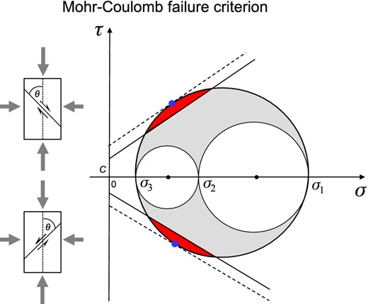
Mohr–Coulomb failure criterion. Quantities τ and σ are the shear and the effective normal stresses, respectively; σ₁, σ₂ and σ₃ are the effective principal stresses. The red area shows all possible orientations of fault planes which satisfy the Mohr–Coulomb failure criterion. The blue dots denote the principal fault planes which are optimally oriented with respect to stress, and C denotes the cohesion. Upper and lower half planes of the diagram correspond to the conjugate faults.

The fault plane is the nodal plane which has the higher value of Coulomb failure stress Δτ. In evaluating Δτ in eq. (10) we need the value of friction μ. Cohesion C and pore pressure p in eq. (11) are not needed, because we are comparing the relative difference of stresses. Friction μ for fractures was measured on rock samples in the laboratory and ranged mostly between 0.6 and 0.8 (Byerlee 1978). The values of friction of faults in the Earth's crust are similar (Vavryčuk 2011) but for some large-scale faults such as the San Andreas fault lower values like 0.2–0.4 have also been reported (Scholz 2002).

Tractions τ and τ_c are always assumed to be positive in eqs (10) and (11) and thus, in principle, it would be sufficient to plot just the upper half plane of the Mohr circle diagram in Fig. 1 (see Jaeger et al.2007, their fig. 4.9; Zoback 2010, his fig. 5.9). The full Mohr circle diagram is obtained by considering a sign for shear traction τ defined in the following way:

\begin{equation} {\rm sign}\left( \tau \right) = {\rm sign}\left( {{\bf N} \cdot {\bf e}^{(3)} } \right), \end{equation}

(12)

where N is the direction of shear traction τ along the fault, and e⁽³⁾ is the direction of the minimum principal stress. Plotting of the full Mohr circle diagram is convenient for distinguishing conjugate faults (see Fig. 1, left-hand plots).

Another way of identifying the fault plane is evaluating the fault instability I proposed by Vavryčuk et al. (2013, their eq. 3):

\begin{equation} I = \frac{{\tau - \mu \left( {\sigma - \sigma _1 } \right)}}{{\tau _c - \mu \left( {\sigma _c - \sigma _1 } \right)}}, \end{equation}

(13)

where τ_c and σ_c are the shear traction and effective normal traction along the optimally oriented fault (Fig. 2, red dot), and τ and σ are the shear traction and effective normal traction along the analysed fault plane (Fig. 2, black dot). Since eq. (13) is independent of absolute stress values, the fault instability I can be evaluated just from friction μ, shape ratio R and from directional cosines n defining the inclination of the fault plane from the principal stress axes. If we scale the reduced stress tensor as follows:

\begin{equation} \sigma _1 = 1,\;\sigma _2 = 1 - 2R,\;\sigma _3 = - 1, \end{equation}

(14)

where positive values mean compression, we get

\begin{equation} \tau _c = \frac{1}{{\sqrt {1 + \mu ^2 } }},\;\sigma _c = - \frac{\mu }{{\sqrt {1 + \mu ^2 } }} \end{equation}

(15)

and consequently

\begin{equation} I = \frac{{\tau - \mu \left( {\sigma - 1} \right)}}{{\mu + \sqrt {1 + \mu ^2 } }}, \end{equation}

(16)

where

\begin{equation} \sigma = n_1^2 + (1 - 2R)\,n_2^2 - n_3^2 , \end{equation}

(17)

\begin{equation} \tau = \sqrt {n_1^2 + (1 - 2R)^2 n_2^2 + n_3^2 - \left[ {n_1^2 + (1 - 2R)n_2^2 - n_3^2 } \right]^2 } . \end{equation}

(18)

Figure 2.

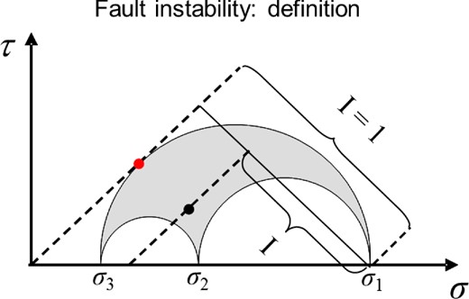
Definition of the fault instability in Mohr's diagram. The red dot marks the tractions on the principal fault characterized by instability I = 1. The black dot marks the tractions of an arbitrarily oriented fault with instability I.

Quantity R is the shape ratio defined in eq. (1) and n is the fault normal expressed in the coordinate system of the principal stress directions. Fault instability I ranges from 0 (the most stable faults) to 1 (the most unstable faults). The most unstable fault is the optimally oriented fault for shear faulting (see Fig. 2, red dot) called the principal fault (Vavryčuk 2011). Note that eq. (16) for the fault instability looks different from that in Vavryčuk et al. (2013, their eq. 6), where positive σ means extension but not compression as in this paper.

4 ITERATIVE STRESS INVERSION

Lund & Slunga (1999) applied the fault instability constraint to the stress inversion of Gephart & Forsyth (1984) and improved its efficiency. Here, we apply this constraint to Michael's method (1984). Since the Gephart & Forsyth algorithm is non-linear and the misfit is sought in a grid, the fault instability constraint can easily be implemented when evaluating the fit for each stress. In contrast to the method of Gephart & Forsyth, Michael's method is linear and implementing the fault instability constraint leads to solving the stress inversion in iterations. First, Michael's method is applied in a standard way without considering any constraint and with no knowledge of the orientation of the fault planes. After finding the principal stress directions and the shape ratio, these values are used for evaluating the instability (16) of the nodal planes for all inverted focal mechanisms. The fault planes are the nodal planes which are more unstable. The orientations of the fault planes found in the first iteration are used in the second iteration performed again using Michael's method. The procedure is repeated until the stress converges to some optimum values.

When evaluating the fault instability using eq. (16), a value of friction μ is needed. As mentioned above, friction on faults most often ranges between 0.2 and 0.8, but its value is usually unknown. Numerical tests revealed, however, that the inversion is rather insensitive to μ, so it is often sufficient to assign some mean value to friction during the inversion, for example, μ = 0.6. Another approach is to run the inversion for several values of friction and adopt the value which produces the highest overall instability of faults for the data inverted. This approach is used in the subsequent synthetic tests as well as in the applications to real data.

5 ACCURACY TESTS

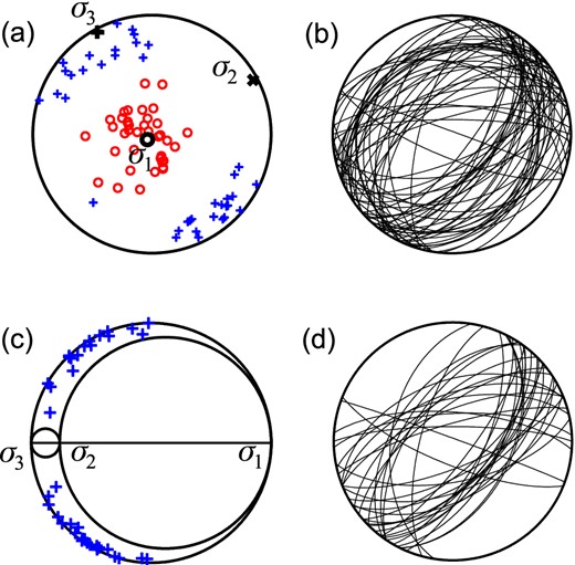
The robustness and accuracy of the iterative stress inversion can be tested using numerical modelling. We present numerical tests performed on sets with a varying number of focal mechanisms ranging from 20 to 200. The focal mechanisms were selected to satisfy the Mohr–Coulomb failure criterion (see Fig. 3). Subsequently, corresponding moment tensors were calculated and contaminated by uniform noise of several levels ranging from 0 to 100 per cent of the moment tensor norm. The norm was calculated as the absolute value of the maximum eigenvalue of the moment tensor (the so-called ‘spectral norm’). The noisy moment tensors were decomposed back into strikes, dips and rakes of noisy focal mechanisms and these mechanisms were inverted for stress. The mean deviations between the true and noisy fault normals and slips attained values from 0° to 35°. Since the inverted focal mechanisms were calculated from moment tensors, the identification of a fault from two nodal planes was ambiguous. The inversion was run repeatedly using 50 realizations of random noise and for two types of sets of focal mechanisms. The first set consisted of focal mechanisms which were projected into both half planes of the Mohr's circle diagram (Fig. 3a). According to Vavryčuk (2011), the P/T axes form a pattern called the ‘two butterfly wings’ (Fig. 3c). The second set consisted of the same number of focal mechanisms but with their variability reduced. The selected focal mechanisms were projected just into the upper half plane of the Mohr's circle diagram (Fig. 3b) and covered just one butterfly wing in the P/T plot (Fig. 3d). The inverted principal stress directions and shape ratios for both data sets and for all realizations of random noise were compared with the true values and the errors were evaluated (see Figs 4 and 5). Similarly, the faults identified from the nodal planes by the inversion were compared with the true ones and the success of the identification was evaluated (see Fig. 6).

Figure 3.

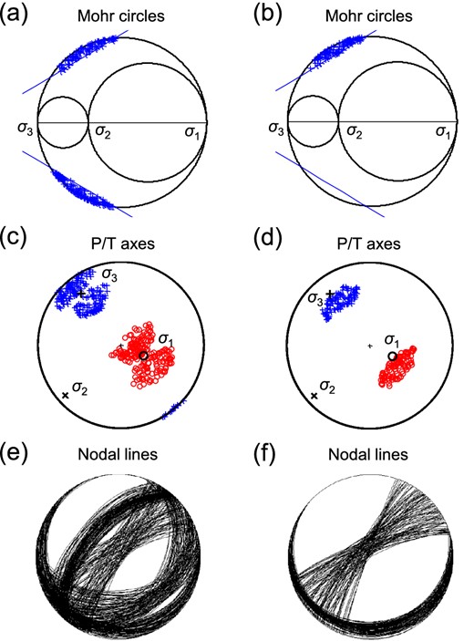
Example of data used in numerical tests of stress inversions. The plots show 200 noise-free focal mechanisms selected to satisfy the Mohr–Coulomb failure criterion. Left/right-hand plots—data set with a full/reduced variety of focal mechanisms. (a, b) Mohr's circle diagrams, (c, d) the P/T axes and (e, f) the corresponding nodal lines. The P axes are marked by the red circles and T axes by the blue crosses in (c) and (d). The P/T axes form the so-called two butterfly wings in plot (c) and one butterfly wing in plot (d), see Vavryčuk (2011). The σ₁, σ₂ and σ₃ stress axes are (azimuth/plunge): 115°/65°, 228°/10° and 322°/23°, respectively. Shape ratio R is 0.7, cohesion C is 0.85, pore pressure p is zero and friction μ is 0.6.

Figure 4.

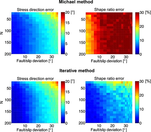
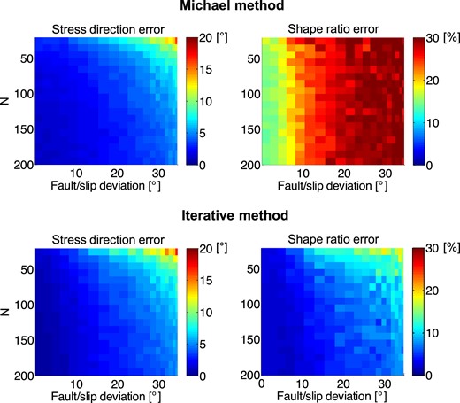
Mean errors of the principal stress directions (left-hand plot) and of the shape ratio (right-hand plot) as a function of the number of focal mechanisms and noise. The data set with a reduced variety of focal mechanisms (one-wing data) is inverted. Upper plots—Michael's method; lower plots—the iterative inversion method. The stress direction error is the average of deviations between the true and retrieved principal stress axes. The errors are further averaged over 50 random realizations of noise. The errors in stress directions are in degrees, the errors in the shape ratio are in per cent.

Figure 5.

The same as for Fig. 4, but for the data set with a full variety of focal mechanisms (two-wing data).

Figure 6.

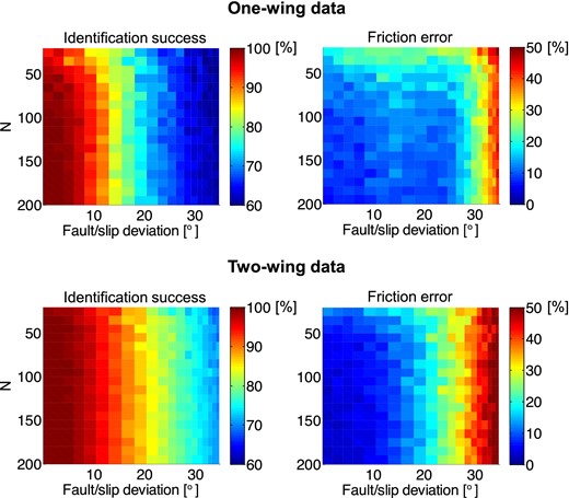
The identification success (left-hand panel) and the errors of friction (right-hand panel) as a function of the number of focal mechanisms and noise. The iterative stress inversion is applied. Upper plots: the data set with the reduced variety of focal mechanisms; lower plots : the data set with the full variety of focal mechanisms. The values are calculated from 50 random realizations of noise. Identification success means the relative number of correctly identified faults.

In order to avoid the sensitivity of the inversion to friction, needed in the instability constraint, the inversion was run repeatedly with friction ranging from 0.2 to 1.2 in steps of 0.05. For each friction, an overall instability of faults identified by the inversion was evaluated, and the friction, which produced the highest overall fault instability, was considered as optimum.

The numerical tests indicate that the accuracy of the stress inversions varies being dependent on the number of focal mechanisms inverted and on the noise level in the data. Both Michael's and iterative inversions yield satisfactory results for principal stress directions with an average error of less than 12° for a set of 20 noisy focal mechanisms with an error of 20° in the orientation of the fault normal and the slip (see Figs 4 and 5, left-hand plots). For more accurate focal mechanisms or for more extensive data sets, the accuracy is even higher. The difference between both methods is almost invisible, the iterative method being slightly more accurate for data with a low noise level. The reason is simple. If the identification of the fault is unknown, Michael's inversion can never retrieve the true stress directions including the case when a large set of noise-free focal mechanisms is inverted. In contrast, the iterative method removes this deficiency, because the orientations of faults are determined during the iterations. A significant difference between Michael's inversion and the iterative joint inversion appears, however, when determining the shape ratio (see Figs 4 and 5, right-hand plots). The average error of the shape ratio is almost 20 per cent for Michael's inversion even when a large number of noise-free focal mechanisms is inverted. When inverting noisy focal mechanisms, this error is even higher. The iterative method yields an average error of less than 10 per cent except for the inversion of a low number of very noisy focal mechanisms.

In addition, the iterative method is capable of recognizing the faults in the focal mechanisms and of estimating the overall friction on the faults. Fig. 6 (left-hand plots) indicates that the success rate in fault identification is higher than 85 per cent if one-wing noisy focal mechanisms with an average error of 15° are inverted. In case of two-wing focal mechanisms, the success rate is as much as 90 per cent. The value of friction is determined with an accuracy of 10–15 per cent for the same type of data (Fig. 6, right-hand plots).

6 APPLICATION TO DATA

6.1 Central Crete

The efficiency of the iterative joint inversion was verified on the data from central Crete analysed previously by Angelier (1979) and Michael (1984, 1987). The data represent field measurements of 38 fault orientations and slip directions (slickenslides), so the identification of faults and auxiliary nodal planes in the focal mechanisms is known. In the stress inversion, we modified the input data by randomly selecting the faults from the two nodal planes and checked whether the iterative procedure identified the correct fault planes.

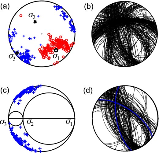
Fig. 7 shows the P/T axes and nodal lines of the input focal mechanisms together with the results of the stress inversion. The retrieved maximum compression is almost vertical (Fig. 7a) and Mohr's circle diagram indicates (Fig. 7c) that the input data cover both butterfly wings. The fault planes (Fig. 7d) were successfully identified in 36 of 38 cases. The shape ratio R was 0.88 and the optimum friction was 0.75. The alternative definition of the shape ratio used by Michael (1984), ϕ = (σ₂ − σ₃)/(σ₁ − σ₃), yields a value of 0.12 identical with the result reported by Michael (1984).

Figure 7.

Iterative inversion for stress using the central Crete data (Angelier 1979; Michael 1984, 1987). (a) P/T axes with retrieved principal stress directions, (b) nodal lines, (c) Mohr's circle diagram with positions of faults (blue plus signs) and (d) faults identified by stress inversion. The P and T axes in (a) are marked by red circles and blue plus signs, respectively.

For analysing the uncertainties in the principal stress directions and in the shape ratio, the stress inversion is run repeatedly with noisy focal mechanisms. We calculated 1000 realizations of noise. The average error in the orientation of faults and slips is assumed to be equally 6°. This value is somewhat arbitrary because we do not know the actual accuracy of the input data. Since we are comparing the efficiency of two inversion methods, a more accurate estimate of the error in focal mechanisms is not vital for our purposes.

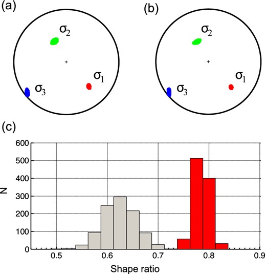
Table 1 and Fig. 8 indicate that the principal stress directions are determined with a similar accuracy regardless of whether the faults are randomly selected from nodal planes (Fig. 8a) or correctly identified by the inversion (Fig. 8b). The behaviour of the shape ratio is, however, remarkably different. Data with randomly selected faults yield a broad distribution of the shape ratio with its maximum significantly biased as compared to the inversion with correctly selected faults. The maximum error is 44 and 12 per cent for randomly and correctly selected faults, respectively.

Figure 8.

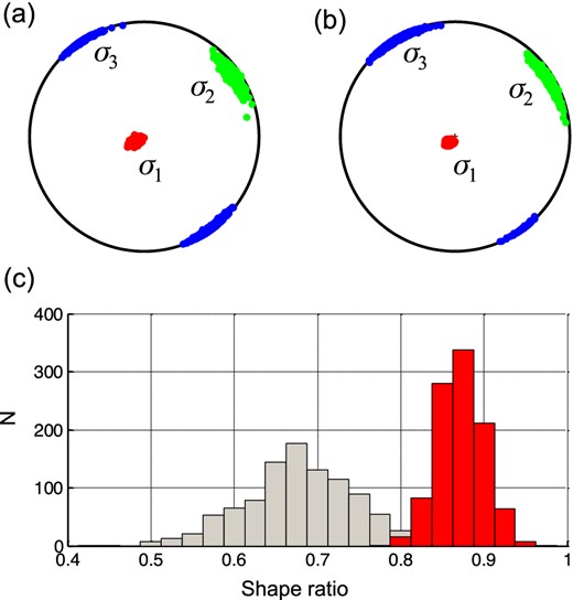
Confidence limits of the principal stress directions retrieved by the Michael method (a) and by the iterative method (b) and histograms of the shape ratio (c). Red, green and blue colours in (a) and (b) correspond to the σ₁, σ₂ and σ₃ stress directions, respectively. The grey and red histograms in (c) define the distributions of the shape ratio calculated using Michael's method and the iterative method, respectively.

Table 1.

Results of stress inversions.

Method	σ1 Azimuth/plunge	σ2 Azimuth/plunge	σ3 Azimuth/plunge	R
Central Crete
Michael's inversion	241.8°/82.7° ± 7.0°	51.3°/7.2° ± 27.8°	141.5°/1.3° ± 27.7°	0.77 ± 44 per cent
Iterative inversion	220.3°/84.7° ± 4.7°	62.5°/4.9° ± 21.5°	332.4°/2.0° ± 21.5°	0.88 ± 12 per cent
West Bohemia
Michael's inversion	137.7°/34.8° ± 3.5°	332.8°/52.9° ± 6.5°	233.1°/7.3° ± 6.4°	0.66 ± 23 per cent
Iterative inversion	138.6°/35.1° ± 2.4°	332.1°/54.1° ± 6.4°	233.1°/6.5° ± 6.0°	0.78 ± 6 per cent

Note: The errors are the maximum differences between the results calculated for the noise-free and noisy focal mechanisms with 1000 random realizations.

6.2 West Bohemia swarm area

The iterative joint stress inversion is further exemplified on the data from the 2008 earthquake swarm in West Bohemia, Czech Republic (Fischer et al.2010; Vavryčuk 2011; Davi & Vavryčuk 2012; Vavryčuk et al.2013; Fischer et al.2014). Since the micro-earthquakes were recorded by many local seismic stations with good focal sphere coverage, they represent a high-quality data set suitable for retrieving the focal mechanisms and tectonic stress very accurately.

We selected 167 micro-earthquakes recorded at all WEBNET stations with a good signal-to-noise ratio and applied the moment tensor inversion of vertical components of the direct P waveforms. The Green functions were calculated using the ray method (Červený 2001) and the full moment tensors were determined using the generalized linear inversion in the time domain (Vavryčuk & Kühn 2012). The accuracy of the focal mechanisms was assessed by repeated inversions using noisy input data and biased locations (epicentres with an error of 250 m and depth with an error of 500 m). The mean errors in the orientations of the fault normal and slip direction were estimated to be equally about 6°.

The tectonic stress in the focal zone was calculated from the 167 focal mechanisms (Fig. 9) using the Michael (1984) and iterative joint stress inversions (see Table 1). The errors were calculated similarly as for the central Crete data by inverting noisy focal mechanisms. We calculated 1000 realizations of noise which produced an accuracy similar to that of the retrieved focal mechanisms (mean error of 6° in the fault normal and slip direction). In the iterative stress inversion, the final stress was obtained after three to four iterations. The fault planes cover both butterfly wings (Fig. 9c). The stress is characterized by the horizontal σ₃ axis, the σ₁ and σ₂ axes significantly deviating from both the horizontal and vertical directions (Fig. 9a). The directions of the principal stress axes and their uncertainties are almost identical for Michael's and the iterative stress inversions (Figs 10a and b). The main difference between both methods is in the shape ratio. Michael's method yields a biased value of the shape ratio with a high error (Fig. 10c), similarly as in synthetic tests. The iterative inversion yields accurate directions of the principal stresses as well as an accurate value of the shape ratio (Table 1). Moreover, the iterative inversion is able to identify the fault planes. As expected, the fault planes cluster in the area of the validity of the Mohr–Coulomb failure criterion (Fig. 9c). The retrieved orientations of the faults were confirmed by analysing foci clustering (Vavryčuk et al.2013). The foci clustered along two fault systems (Fig. 9d) referred to as the principal faults in the region (Vavryčuk 2011, his fig. 10). The optimum overall friction found in the inversion was 0.85.

Figure 9.

The same as Fig. 8 but for the West Bohemia data. The blue lines in (d) define the principal faults in the West Bohemia region identified from foci clustering (see Vavryčuk et al.2013).

Figure 10.

The same as Fig. 8 but for the West Bohemia data.

7 DISCUSSION

Michael's method is quite fast and accurate when retrieving directions of the principal stresses. It yields a reasonable accuracy even for randomly selected fault planes in focal mechanisms. However, the accuracy of the shape ratio is significantly lowered when the fault planes are not correctly chosen. The value of the shape ratio is very approximate even if a large number of accurate focal mechanisms is inverted. Hence the shape ratio is more sensitive to the correct choice of the fault than the principal stress directions and substituting the faults by the auxiliary nodal planes introduces high errors.

An accurate value of the shape ratio can be calculated by the iterative joint inversion for stress and fault orientations. In this inversion, the fault instability constraint is applied and the fault is identified with that nodal plane which is more unstable and thus more susceptible to faulting. Incorporating the fault instability constraint into the inversion leads to an iterative procedure. Instead of calculating the stress in one step, the stress must be calculated in iterations. In the first iteration, Michael's method is run with randomly selected fault planes. In the second and higher iterations, Michael's method is run with the fault planes identified by the instability constraint. The numerical tests show that the procedure converges after three to four iterations. Since principal stress directions are well retrieved even in the first iteration, the subsequent iterations identify the fault planes and improve mainly the shape ratio. This is the reason why the convergence is so fast.

When analysing real data sets, the uncertainties of the retrieved stress directions, the shape ratio, the fault selection and overall friction on faults are not calculated by the bootstrap method as proposed by Michael (1987). Here the uncertainties are calculated as the maximum differences between the results of the inversion for noise-free and noisy data with 1000 noise realizations. This method is convenient for several reasons. First, it can take into account the case when some nodal planes are more uncertain than the others by specifying differently noise levels for the fault orientations and slip directions. And secondly, the obtained uncertainties are more realistic. For example, the histogram of the shape ratio can be quite broad (Figs 8c and 10c) and the true values need not lie necessarily close to its maximum.

The efficiency of the iterative inversion was tested on the data from central Crete and from West Bohemia, Czech Republic. For both data sets, the method worked well and produced a significantly more accurate shape ratio than the inversion of the focal mechanisms with randomly selected faults. When plotting Mohr's circle diagram, the faults identified by the inversion displayed high fault instability and concentrated in the area of validity of the Mohr–Coulomb failure criterion. This is a clear indication that the data are consistent with the fault instability model and that the application of the iterative stress inversion is appropriate. If the faults identified by the inversion do not display high instability, the fault instability model is probably not fully suitable, and the results of the iterative inversion could be less reliable. This can be caused either by high errors in the focal mechanisms or by a more complicated stress field or tectonic conditions in the studied area.

Michael's method is quite popular and has been used in several stress inversion codes such as SATSI (Hardebeck 2006; Hardebeck & Michael 2006) or its Matlab modification MSATSI (Martínez-Garzón et al.2013, 2014; Ickrath et al.2014). Since the iterative stress inversion is based on Michael's method, it can easily be implemented in these codes enhancing their accuracy. The Matlab code of this inversion called STRESSINVERSE is provided on the web page (http://www.ig.cas.cz/stress-inverse, last accessed 27 June 2014).

I wish to thank Björn Lund for a constructive and detailed review, Andrew Michael for providing me with data from central Crete, and Julie Vavryčuková for help with coding in Matlab. The study was supported by the Grant Agency of the Czech Republic, Grant No. 210/12/1491.