Vertical land motion and sea level change in Macaronesia

Abstract

This study addresses long-term sea level variability in Macaronesia from a holistic perspective using all available instrumental records in the region, including a dense network of GPS continuous stations, tide gauges and satellite observations. A detailed assessment of vertical movement from GPS time series underlines the influence of the complex volcano-tectonic setting of the Macaronesian islands in local uplift/subsidence. Relative sea level for the region is spatially highly variable, ranging from −1.1 to 5.1 mm yr⁻¹. Absolute sea level from satellite altimetry exhibits consistent trends in the Macaronesia, with a mean value of 3.0 ± 0.5 mm yr⁻¹. Typically, sea level trends from tide gauge records corrected for vertical movement using the estimates from GPS time series are lower than uncorrected estimates. The agreement between satellite altimetry and tide gauge trends corrected for vertical land varies substantially from island to island. Trends derived from the combination of GPS and tide gauge observations differ by less than 1 mm yr⁻¹ with respect to absolute sea level trends from satellite altimetry for 56 per cent of the stations, despite the heterogeneity in length of both GPS and tide gauge series, and the influence of volcanic-tectonic processes affecting the position of some GPS stations.

Global change from geodesy, Satellite geodesy, Sea level change; Atlantic Ocean

1 INTRODUCTION

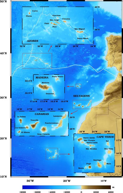
Sea level change associated with climate change represents a major concern worldwide, particularly for coastal areas and islands. The group of archipelagos forming Macaronesia is among the regions threatened by the impact of sea level change. Macaronesia includes the Azores, Madeira, Canaries and Cape Verde archipelagos, encompassing a total of 32 islands, many islets, and reefs (Mitchell-Thomé 1976). Geographically, Macaronesia extends approximately from latitudes 14.8°N to 39.7°N and from longitudes 13.4°W to 30.9°W (Fig. 1). All the islands are of volcanic origin, corresponding to intraplate hotspots attributed to the action of mantle plumes (Madeira, Canaries and Cape Verde) or related to interplate magmatism at a triple junction (Azores) (Madeira & Ribeiro 1990; Marques et al.2013; Carracedo et al.2015).

Figure 1.

Location of the Macaronesian archipelagos. Global topography from SRTM_15_PLUS (Becker et al.2009) and plate boundaries from Argus et al. (2011).

As a result of their geodynamic setting, origin and morphology, the Macaronesian islands are prone to geological hazards, such as volcanic eruptions, earthquakes and landslides. The consideration of these natural processes is important, as they may influence the instrumental records used to estimate vertical land motion and therefore sea level variability. There has been volcanic activity in recent centuries in all the Macaronesian archipelagos, with the exception of Madeira, which is presently in a dormant volcanic stage (Brum da Silveira et al.2010). In the Azores the latest eruption was first detected in December 1998 off the Terceira Island and persisted until August 2001 (Gaspar et al.2003). In the Canary archipelago the latest eruption occurred in October 2011 off the southernmost tip of El Hierro. In Cape Verde the latest eruption took place in the island of Fogo from the end of November 2014 to early February 2015 (Worsley 2015). In what regards seismicity and neotectonic surface deformation, Azores is the archipelago more prone to this kind of events due to its location on a triple junction, with several destructive earthquakes in post-settlement times (Madeira 2005; Trota 2009).

Despite the scientific and societal relevance of sea level change in Macaronesia, a holistic assessment of sea level variability in the region using all the available instrumental records (tide gauges, GPS, and satellite altimetry) is still nonexistent. Detailed studies have been performed for specific islands in the Canary archipelago (e.g. Marcos et al.2013; Pérez-Gómez et al.2015), or in São Miguel Island, in the Azores archipelago (Ng et al.2014), but the poor sampling of the area and the lack of long continuous tide gauge records hinders a regional assessment of sea level change. Furthermore, reliable estimates of vertical land motion, which are crucial to derive long-term sea level trends, require also long time series of GPS measurements, since glacial isostatic adjustment (GIA) model predictions of vertical motion are unsuitable in tectono-volcanically active regions as is the case of Macaronesia. The present study addresses vertical land motion based on GPS data from a comprehensive set of continuous stations operating in Macaronesia. The resulting estimates are used to correct sea level trends from tide gauge records in the region, and further compare them with absolute sea level trends from satellite altimetry time series for a synergistic assessment of sea level change in the Macaronesian region. The simultaneous analysis of tide gauge, GPS and satellite altimetry observations is crucial for a more throughout understanding of sea level variability not only in Macaronesia but also in other regions with a complex geodynamic setting.

2 DATA SETS

2.1 GPS

GPS raw data sets comprise data from permanent stations maintained by different public and private sources, conveniently available through the Canary GNSS Centre (Romero et al.2007; Romero et al.2009), and data from more than 300 global tracking stations, largely from the International GNSS Service (IGS) (Dow et al.2009) and EUREF (Bruyninx et al.2012) permanent networks.

GPS data were processed using the GAMIT/GLOBK software package (Herring et al.2015a,b), for a 20 yr period (1996.0–2016.0). First the full set of GPS data was organized and processed into different subnetworks, sharing a few common sites to ensure the necessary ties, providing, among other parameters, a series of daily estimates of loosely constrained station coordinates, along with the associated variance–covariance matrices (the main settings used in data processing are listed in Table 1). Second, the daily solutions of the different networks were used as quasi-observations and combined to estimate a consistent set of coordinates for all stations (see Mendes et al.2013 for more details), from which we generated the GPS time series for the region of interest.

Table 1.

Main data processing settings used in GAMIT.

Observations	Double-differenced, ionosphere-free linear combination of L1 and L2 carrier phases
Elevation cut-off angle	10°
Observations weight	Elevation-angle dependent
Antenna phase centre variations	IGS absolute models for satellite and receiver antennas
Neutral atmosphere refraction	A priori zenith delays from GPT2 model (Lagler et al.2013), mapped with the VMF mapping functions (Boehm et al. 2006); station zenith delays corrections estimated at each station at 1 hr interval; station gradients parameters in north–south and east–west directions at 24 hr interval
Solid earth tides	IERS Conventions 2010 (Petit & Luzum 2010)
Ocean tide loading	Computed using the FES2004 ocean tide model (Lyard et al.2006)
Orbits	ESA/ESOC orbits (Springer et al. 2014) (including IGS 2nd data reprocessing for older data), expressed in ITRF2008 (Altamimi et al.2011)
Earth orientation	International Earth Rotation and Reference Systems Service (IERS) Bulletin B (US Naval Observatory (USNO) for the most recent data processing)
Interannual variation in polar motion	The effects of deformation due to interannual variation in polar motion (King & Watson, 2014) were not taken into account.
Reference Frame	ITRF2008 (Altamimi et al., 2011)

There are three distinct groups of GPS time series: (1) time series of stations with a long historic record, but with very low data completeness; (2) time series of stations with almost continuous data but with a short period of operation; (3) time series of stations with very long records and good data completeness. For the second group, only time series for stations operating for at least ∼5 yr were selected. This data span is essentially twice the value that Blewitt & Lavallée (2002) recommend to be adopted as the standard minimum for high accuracy applications (2.5 yr), but as it will be discussed, even trends derived from these longer time series are every so often far from being robust.

2.2 Tide Gauges

We used monthly time series of relative sea level from tide gauges in the Macaronesia region from the Permanent Service for Mean Sea Level (PSMSL; Holgate et al.2013; PSMSL, 2016), complemented with Research Quality Data daily time series from the University of Hawaii Sea Level Center/National Oceanographic Joint Archive for Sea Level (UHSLC/JASL; Caldwell & Merrifield 2015) in the case of Madeira.

For the sake of consistency with the files disseminated by the PSMSL, we converted the daily series from UHSLC into monthly series, by simply averaging the daily values for each month. For discussion purposes, we will prepend, respectively, UH_ and PS_ to the UHSLC/JASL and PSMSL station identification.

2.3 Satellite altimetry

Satellite altimetry data from January 1993 to December 2015 were extracted from the Radar Altimeter Database System—RADS4 (Scharroo et al.2013). Time series of sea level anomalies for latitude ranging from 14°N to 41°N and longitude ranging 10°W to 35°W were obtained on a regular along-track grid with a 0.25° resolution from the common ground-track missions T/P (cycles 11–364), Jason-1 (cycles 22–258) and Jason-2 (cycles 20–276), resulting in a total of 1952 grid points. Sea level anomalies were computed with respect to the mean sea surface DTU13MSS (Andersen et al.2015). All standard geophysical corrections were applied (Scharroo 2016) except for the inverse barometer correction, which was not applied for consistency between the satellite altimetry data and the tide gauge data. The time resolution for these time series is ∼10 d.

In order to create a grid point to be used to the TG/GPS pair, we considered all the grid points within a degree of latitude and longitude of each tide gauge and computed the mean for such region. The uncertainty for this mean point was computed by error propagation of the uncertainties associated to each grid point estimate. This strategy yields similar results to that of the most correlated grid point or the closest grid point, but is more robust (the correlations between each candidate grid point and the tide gauge were similar and not very strong). These reference grid points are identified in the text by the prefix SA_ prepended to the name of a GPS station in their vicinity.

While satellite altimetry in the open ocean is a mature technique, its application in the coastal zone, despite significant progress in recent years (e.g. Vignudelli et al. 2011) is limited by difficulties associated with the radar altimeter footprint and resulting land contamination in the returned waveforms as well as in the corrections (tides, atmosphere) required to convert the altimeter range into a sea level height measurement.

3 DATA PROCESSING

The reliable estimation of trends and associated uncertainties requires an accurate representation of seasonal and stochastic variability, which are addressed in this section.

3.1 Seasonal model

The seasonal signal in geophysical time series is generally represented by a sum of sinusoids with annual frequency and possibly higher-order harmonics (e.g. semi-annual, quarterly). In the case of GPS series, besides the seasonal signals (solar signals), orbital (draconitic) and tidal signals have also been observed (Ray et al.2008; Davis et al.2012; Tornatore et al.2016). For time series with significant large gaps, the estimation of this seasonal cycle may be unreliable and therefore not advisable, as is the case of the GPS time series for GRAC, FLOR, PLUZ and TGCV. Three different functional models were considered for the time series with good data completeness: a model with only bias and trend (along with offsets, if needed), a model with an additional annual harmonic and a third one with both annual and semi-annual harmonics. The selection of the best model was based on the analysis of the Bayesian Information Criterion (BIC; Schwarz 1978), using in all cases the Generalized Gauss–Markov model for the noise. We concluded from this analysis that, in general, the seasonal cycle is better characterized as a sum of annual and semi-annual harmonics.

For the GPS time series, the amplitudes of the seasonal cycle are very small, ranging from a minimum of 0.5 mm, for station ALDE, to a maximum of 4.7 mm, for station VFDC (Fig. 2). The contribution of surface mass distributions to the seasonal GPS signal is smaller for oceanic islands (Dong et al.2002). Furthermore the contribution from the thermal expansion of the monuments is negligible. Yan et al. (2009) estimated this contribution to be 0.19 mm for PDEL and 0.14 mm for MAS1. The mass loading contribution for the same sites is roughly twice this value, still a small contribution to the observed amplitudes. Mismodelling of certain type of errors may therefore represent the main contribution to the seasonal variation in the Macaronesian sites.

Figure 2.

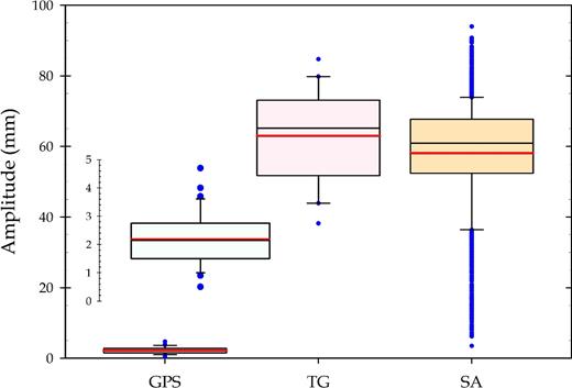
Box-and-whisker representation of the amplitude of the seasonal cycle for the different types of series. A close-up for the GPS series is also shown as inset. The boundaries of the box represent the 25th and 75th percentiles, the thinner and thicker lines within the box marks the median and mean, respectively, and the whiskers below and above the boxes represent the 10th and 90th percentiles. The blue dots mark the outlying points. The large number of outlying points below the 10th percentile is related with the smaller amplitude of the grid points at lower latitudes.

The seasonal amplitude for the satellite altimetry is quite variable for Macaronesia, as shown in Fig. 2, with a significant reduction for low latitudes, except for near-shore and coastal locations (see Fig. 3). The mean value for the 1952 grid points is 58 ± 15 mm, with a marked dominance of the annual component, with amplitude of 52 ± 14 mm.

Figure 3.

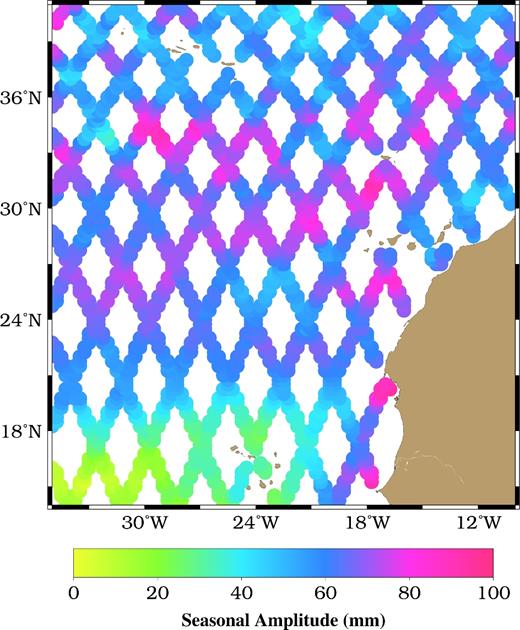
Seasonal amplitude (annual and semi-annual contribution) for SA grid points.

For the tide gauges time series, the amplitude of the seasonal cycle is higher and equally variable (63 ± 13 mm), with a minimum for UH_210 (Santa Cruz das Flores) and a maximum for PS_2051 (Hierro). The semi-annual component of the seasonal cycle is more relevant for the tide gauge than for the satellite altimetry series. The annual component for the TG series represents ∼72 per cent of the seasonal cycle, with a minimum for PS_258 (Ponta Delgada) and a maximum for PS_2024 (Funchal) and PS_1803 (Tenerife). The seasonal cycle for tide gauges is also affected by the seasonal variations of the vertical land motion, but these seasonal cycles are very low in Macaronesia, as mentioned before.

3.2 Stochastic model

It is a well-established fact that the time series of daily GPS position estimates for continuously operating stations are affected by noise uncorrelated in time (white noise) and noise correlated in time (coloured noise; e.g. Zhang et al. 1997; Mao et al. 1999; Langbein 2008; Santamaría-Gómez et al. 2011; Langbein, 2012; Serpelloni et al. 2013). This temporal correlation needs to be properly modelled, in order to derive unbiased trends and realistic uncertainties. Most studies on this subject focused on the choice of the model (normally a combination of white noise and power-law processes) that best describes the noise characteristics of GPS time series. In general, these studies show that the use of a pure white noise model yields velocity uncertainties that are underestimated up to one order of magnitude.

We analysed GPS time series from 39 continuous stations with different noise options using the Hector software package (Bos et al.2013). The tested models were: autoregressive moving average (ARMA), autoregressive fractionally integrated moving average (ARFIMA), Generalized Gauss–Markov (GGM), Power Law (PL) and Flicker Noise (FN), combined with White Noise (WN). For the ARMA and ARFIMA models, we use p = 1 and q = 0 for autoregressive and moving average coefficients, respectively (also represented as AR(1) and ARFIMA(1, d)). Based on the Akaike information criterion (AIC; Akaike 1974) to assess the best noise combination, GGM achieved the best ranking, in agreement with the conclusions of Xu (2016). This combination was the best performing model for ∼49 per cent of our series, followed by PL (∼33 per cent); nonetheless, for some series, the differences in AIC for the two models are very small, showing therefore no clear preference for any of the models. The FN model was not preferred for any of our time series. Uncertainties are similar for the ARFIMA and PL models (mean ratio of 4.6 and 4.8 with respect to the WN model), lowest for ARMA (mean ratio of 1.6), and highest for FN (∼12.4).

For the analysis of the SA and TG time series, we considered only the ARFIMA, ARMA, GGM, and PL noise models. The results for the 1952 SA time series ranked the ARFIMA (38.6 per cent), GGM (36.5 per cent), and ARMA (24.9 per cent) as the best models and almost equally preferred, with very small differences in the AIC values (a mean percentage difference of just 0.01 per cent between ARFIMA and GGM). These models have a mean increase factor of 2.1 (GGM and ARMA) and 3.0 (ARFIMA) in the uncertainties with respect to WN.

Similar conclusions were drawn by Bos et al. (2014), who have also tested a fifth order autoregressive model, in their analysis of SA global sea level data sets. Using the BIC criterion, they found out that the ARFIMA and the GGM models were equally preferred, followed by the AR(5), with AR(1) ranking last. The use of the AR(5) model was proposed by Hughes & Williams (2010) in the analysis of weekly sea surface height (SSH) observations as the model that best described SSH at most locations in the ocean.

As regards the increase in the rate uncertainty, Wöppelmann & Marcos (2016) also noted a factor between 2 and 3 when taking into account the temporal correlation in the analysis of SA data. Bos et al. (2014) refer that the use of AR(1) underestimates the rate uncertainties by a factor no less than 1.3.

Similar results were obtained in the analysis of the TG time series. The best ranked model was the GGM (40 per cent of the series), but with no clear superiority over the ARMA (30 per cent) and ARFIMA (25 per cent) noise models. These results are in agreement with the conclusions of a larger study by Bos et al. (2014). As regards the uncertainties, GGM and ARFIMA yield identical values (corresponding to ratios of 2.2 and 2.3 with respect to the white noise model, respectively), being ∼1.2 times higher than the more optimistic uncertainties associated with the ARMA noise model.

Hay et al. (2013) investigated the use of AR processes of different order to characterize the interannual noise for TG to conclude that the AR(5) model is well adapted for stations with more than 50 years’ worth of data whereas the AR(3) is more adapted to the other cases.

4 VERTICAL MOVEMENTS

4.1 GPS

The GPS-derived vertical trends obtained using the GGM stochastic model are presented in Table 2. Whenever available, these are compared with GPS trends presented in previous studies, and with the online solutions provided by the Scripps Orbit and Permanent Array Center (SOPAC, http://sopac.ucsd.edu) and by the Jet Propulsion Laboratory (JPL, http://sideshow.jpl.nasa.gov/post/series.html). The solutions provided by JPL are particularly interesting, as they are derived using a different suite of programs (GIPSY-OASIS) and a different estimation strategy (precise point positioning) (Zumberge et al.1997). Trends obtained from SOPAC correspond to the unfiltered solutions. For the online solutions, the quoted trends refer to the solutions available on March 2017.

Table 2.

GPS trends (⁠|${\dot{\rm U}_{\rm GPS}}$|⁠, in mm yr⁻¹) and respective uncertainties (σ, in mm yr⁻¹).

SITE	Location	λ	φ	Δt	CI	|${{{\bf \dot{U}}}_{{{\bf GPS}}}}$|	σ
1-FLOR	Flores	− 31.1308	39.4575	6.8	23	− 1.55	0.47
2-FLRS	Flores	− 31.1264	39.4538	7.5	96	− 1.52	0.18
3-GRAC	Graciosa	− 28.0291	39.0909	5.3	16	− 1.17	0.39
4-AZGR	Graciosa	− 28.0229	39.0879	7.5	91	− 0.43	0.48
5-TERC	Terceira	− 27.1530	38.7190	7.3	91	− 4.00	0.15
6-PTRP	Pico	− 28.3860	38.4196	5.6	83	− 3.04	0.17
7-PIED	Pico	− 28.0325	38.4138	7.2	89	− 2.38	0.13
8-FRNS	São Miguel	− 25.3082	37.7693	8.0	92	− 1.36	0.29
9-PDEL	São Miguel	− 25.6628	37.7478	15.7	94	− 1.97	0.12
10-VFDC	São Miguel	− 25.4357	37.7151	6.4	85	− 0.96	0.34
11-PSTO	Porto Santo	− 16.3352	33.0598	5.9	85	− 1.12	0.28
12-PAUL	Madeira	− 17.1973	32.8232	4.0	76	− 0.74	0.26
13-STNA	Madeira	− 16.8869	32.8102	5.7	85	− 1.17	0.17
14-FUNC	Madeira	− 16.9076	32.6479	5.5	95	− 1.09	0.12
15-IMMA	Madeira	− 16.8922	32.6477	9.9	76	0.49	0.27
16-HRIA	Lanzarote	− 13.4851	29.1452	5.7	90	− 2.08	0.17
17-TIAS	Lanzarote	− 13.6543	28.9521	6.9	97	− 2.31	0.44
18-YAIZ	Lanzarote	− 13.7655	28.9518	5.7	96	− 2.08	0.26
19-LPAL	La Palma	− 17.8938	28.7639	14.5	97	− 1.16	0.20
20-MAZO	La Palma	− 17.7794	28.6057	5.1	86	− 1.59	0.30
21-OLIV	Fuerteventura	− 13.9287	28.6104	4.7	91	− 1.54	0.24
22-ANTI	Fuerteventura	− 14.0139	28.4233	5.6	91	− 1.22	0.56
23-TARA	Fuerteventura	− 14.1152	28.1941	5.1	83	− 2.54	0.27
24-MORJ	Fuerteventura	− 14.3596	28.0518	4.7	76	− 0.30	0.39
25-TENE	Tenerife	− 16.3138	28.4798	4.8	85	0.05	0.23
26-TN01	Tenerife	− 16.2412	28.4772	8.5	82	− 0.80	0.17
27-GRAF	Tenerife	− 16.2679	28.4538	5.5	95	− 0.22	0.52
28-TN02	Tenerife	− 16.5508	28.4183	8.6	95	− 1.24	0.35
29-IZAN	Tenerife	− 16.4997	28.3081	7.3	96	− 2.26	0.13
30-STEI	Tenerife	− 16.8155	28.2977	5.7	90	− 1.61	0.46
31-SNMG	Tenerife	− 16.6154	28.0965	5.5	97	− 1.49	0.20
32-TN03	Tenerife	− 16.7185	28.0473	8.1	95	− 1.98	0.25
33-PLUZ	Gran Canaria	− 15.4076	28.1467	6.6	43	− 1.50	0.24
34-ULP1	Gran Canaria	− 15.4560	28.0700	6.8	85	− 1.52	0.24
35-TERR	Gran Canaria	− 15.5484	28.0595	6.0	95	− 1.98	0.25
36-ALDE	Gran Canaria	− 15.7803	27.9847	5.7	93	− 1.79	0.25
37-AGUI	Gran Canaria	− 15.4458	27.9039	5.7	86	− 1.06	0.35
38-GMAS	Gran Canaria	− 15.6343	27.7648	10.5	96	0.07	0.24
39-MAS1	Gran Canaria	− 15.6333	27.7637	20.0	95	− 0.79	0.13
40-ARGU	Gran Canaria	− 15.6814	27.7610	5.1	91	− 3.05	0.27
41-ALAJ	La Gomera	− 17.2411	28.0638	5.0	85	− 0.67	0.36
42-TGCV	Sal	− 22.9828	16.7548	14.6	24	− 1.06	0.19

Note: λ, longitude (°); φ, latitude (°); Δt, length of the series (years); CI, completeness index (per cent).

In order to evaluate how reliable the trends obtained using the complete time series are, an analysis of the variation of the trends in the last 2 yr is performed. Using the same processing strategy, we looked at the variation in trend since 2014, as new monthly data are included in the estimation process and new cumulative solutions are generated, in a total of 24 solutions. For stations with the shortest time series, it is assured that they have at least ∼3 yr of data. Fig. 4 shows the range of trends during the latest 2 yr (2014–2015) and 1 yr (2015) periods, and the trend uncertainty corresponding to the full time series solution. A large number of stations show a 1 yr range in trend that is below that uncertainty, a good indication of reliability. The stations for which the 1 yr variation exceeds that uncertainty have generally shorter time series, with some exceptions, such as AZGR (to be discussed later), FUNC and TERC. In the following section we discuss in more detail the derived GPS vertical trends for the different archipelagos.

Figure 4.

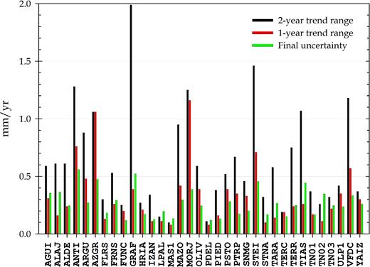
Trend range during the latest 2 yr and 1 yr periods and uncertainty for the full time series solution. Range is the difference between the maximum and minimum trends obtained at each monthly cumulative solution. Final uncertainty is plotted at the one-sigma level.

4.1.1 Madeira archipelago

The station with the longest record in Madeira, IMMA, shows uplift (0.49 ± 0.27 mm yr⁻¹), in opposition to the remaining stations in the archipelago. The station FUNC, located less than 2 km away (Fig. 5), presents a rate of −1.09 ± 0.12 mm yr⁻¹.

Figure 5.

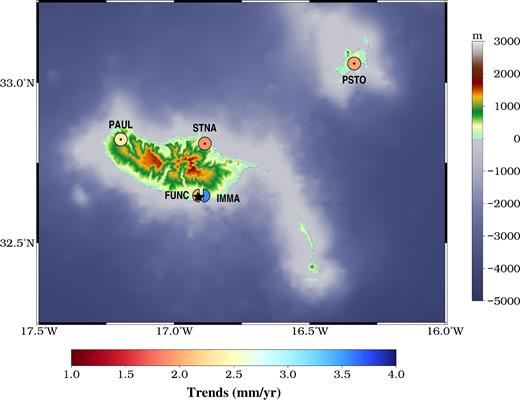
GPS trends (circles/semi-circles) and site locations for GPS and tide gauges (stars) in the Madeira archipelago.

There is an excellent agreement between the GPS trends for FUNC, STNA and PSTO. Subsidence rate for PAUL is slightly lower, but this difference is not significant, due to the larger uncertainty, and may be due to the fact that PAUL has several data gaps, and a shorter time series. The trend for FUNC is very robust with no significant change in the last 2 yr. Trends for FUNC provided by SOPAC and JPL are respectively −1.4 ± 1.2 mm yr⁻¹ and −0.41 ± 0.46 mm yr⁻¹, in agreement within the stated uncertainties. The ULR6a solution (http://www.sonel.org) is −1.10 ± 0.29 mm yr⁻¹, identical to our estimate (the 2016 ULR6a solution covers the period 1995.0–2013.9 and will be used to update the values presented in Santamaría-Gómez et al. 2012). Due to the high level of agreement of trends for FUNC and the remaining stations in the island, we speculate that the uplift at IMMA is likely a local effect, possibly related to wet soil expansion, as the station stands on weathered trachytic air-fall pumice lapilli layers and hydrovolcanic fine ash beds (Brum da Silveira et al.2010).

4.1.2 Azores archipelago

The estimate for FLRS (Flores) of −1.52 ± 0.18 mm yr⁻¹ is in fair agreement with SOPAC's (−1.8 ± 1.0 mm yr⁻¹) and JPL's estimate (−1.06 ± 0.41 mm yr⁻¹), but SOPAC's trend has a very large uncertainty. The variation in trend in the last 2 yr is not significant. Our trend for FLRS is also in excellent agreement with that obtained for the now discontinued station FLOR (−1.55 ± 0.47 mm yr⁻¹), a relevant fact, as the series span different periods of operation.

TERC (Terceira) presents the highest subsidence rate of the Azores archipelago (4.00 ± 0.15 mm yr⁻¹). This high value is consistent with previous published values for nearby stations observed in campaign mode (Trota 2009; Miranda et al.2012; Marques et al.2015; Rodrigues 2015), despite the different time spans of such studies. These present-day GPS trends differ markedly from estimated long-term vertical movements (Quartau et al.2014). The differences between the geological and GPS derived rates can be explained by the fact that they correspond to different timescales and that the short-term contemporary rates could be influenced by episodic tectonic and volcanic processes (Miranda et al.2012; Quartau et al.2014).

The trends for the two stations located in Pico (PIED and PTRP) are still not stable. By the end of 2015, the trends are distinct (difference of ∼0.7 mm yr⁻¹), but the subsidence rate in the last 2 yr is increasing ∼0.2 mm yr⁻¹ for PIED, whereas the subsidence rate for PRTP is decreasing by ∼0.3 mm yr⁻¹. Extending the time series is crucial to determine if local deformation is taking place in Pico and to determine robust estimates of subsidence rate.

For the other stations in the Azores archipelago (AZGR, PDEL, FRNS and VFDC) time series of the daily height component of position are presented in Fig. 6.

Figure 6.

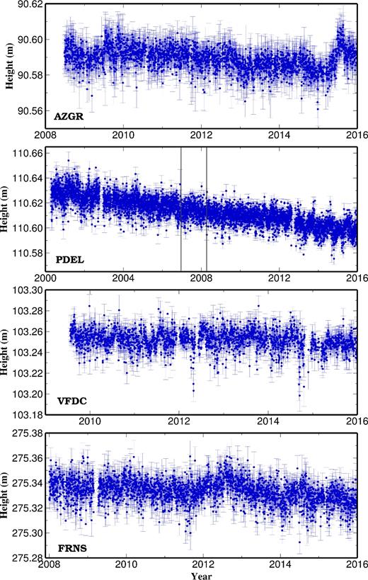
Daily GPS height time series for stations AZGR, PDEL, VFDC and FRNS. Vertical lines for PDEL mark the epochs of estimation of offsets in the series.

We determined the trends for AZGR (Graciosa) using cumulative solutions in a monthly basis covering a 5 yr (2011–2016) period (Fig. 7). There is a clear change in the subsidence rate from June 2015 forward. By the end of June, the subsidence rate for AZGR was 1.21 ± 0.27 mm yr⁻¹; ever since, this rate lowered ∼0.8 mm yr⁻¹. The cause of this change in the height time series is still unclear, as the station did not suffer any change of hardware. This could represent an episode of volcanic unrest (inflation), since an increase in seismic activity was also observed in the region during the same period.

Figure 7.

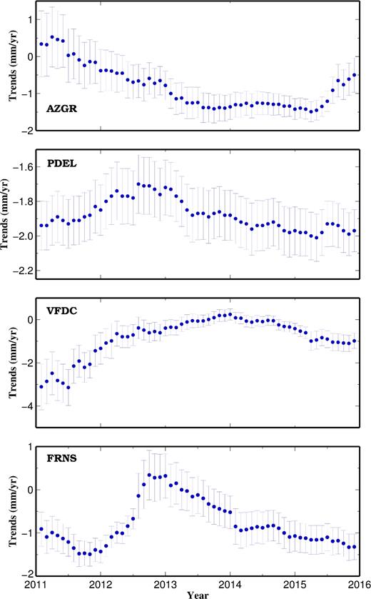
Variations in trend for GPS station AZGR, PDEL, VFDC and FRNS (range is the difference between the maximum and the minimum trends obtained at each month for the last 5 yr).

We analysed data for three permanent stations in São Miguel (Fig. 8): PDEL, FRNS and VFDC. PDEL is the station with the longest record and the most robust solution. There is a large range of estimates for PDEL station, as shown in Table 3. In addition to GPS, PDEL has a DORIS (Willis et al.2010) station (PDMB) located in the same building. We used the DORIS time series of weekly coordinates produced by the International DORIS Service (IDS) Combination Center, available at the CDDIS (https://cddis.nasa.gov), corresponding to solution ‘ids16wd04’, and computed the trend using the same seasonal and stochastic model used in the analysis of GPS data. We obtained a trend of −1.87 ± 0.66 mm yr⁻¹, in agreement with that derived for GPS, but with larger uncertainty. The different time span for the different studies and the strategy to handle breaks in the series (need of estimating offsets) may explain the variety of results in GPS solutions. Our GPS estimate is in excellent agreement with the solutions presented by Wöppelmann et al. (2009) and Rudenko et al. (2013).

Figure 8.

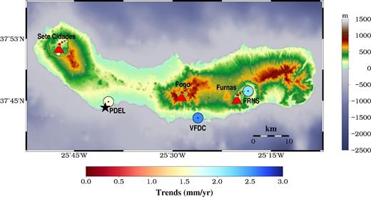
GPS trends (circles) and site locations for GPS and tide gauge (star) in São Miguel Island. Also shown the locations of active central volcanoes (triangles).

Table 3.

Trend estimates (in mm yr⁻¹) for PDEL (São Miguel).

	W2009a	R2013b	SG2012c	SOPAC	JPL	This study
PDEL	−1.90 ± 0.22	−2.08 ± 0.03	−1.51 ± 0.16	−1.1 ± 0.2	−1.69 ± 0.35	−1.97 ± 0.12

a

^aWöppelmann et al. (2009).

^bRudenko et al. (2013).

^cSantamaría-Gómez et al. (2012) (ULR6a solution).

The trends for FRNS and VFDC need some additional discussion. These two stations are characterized by a change in trends in the most recent years. We determined the trends for three stations in São Miguel in a monthly basis, for the period 2011–2016 (Fig. 7). The island experienced events of volcanic unrest in the Fogo-Congro area (Trota 2009; Okada et al. 2015) and these changes in trends are a reflex of the adjustment of the stations to inflation-deflation processes (PDEL is not affected, as it is located farther away from these active volcanic systems). In the last 2 yr the trends for FRNS and VFDC are varying at a rate of ∼0.3 mm yr⁻¹ and ∼0.7 mm yr⁻¹, respectively. If we look at trends since 2011 for these two stations, we can observe a change after September 2011 (see also Fig. 6), corresponding to the initiation of an intense (volcano-tectonic) earthquake swarm that ended in February 2012 (Okada et al.2015; the observed lag is expected, as trends react slower than changes in positions); in the case of FRNS, this change in trend is also accompanied by a significant change in the uncertainty. Okada et al. (2015) did not investigate the vertical component of these stations, but the observed changes in the horizontal components of position are well correlated with the changes in the vertical component. As both stations seem to continue their process of relaxation after the event of volcano-tectonic unrest, the values for their trends need to be taken into account with caution.

4.1.3 Cape Verde archipelago

TGCV is a station covering a long period (almost 15 yr), but with a degree of completeness of only 25 per cent. The trend for TGCV is −1.06 ± 0.19 mm yr⁻¹. JPL estimate is −1.38 ± 0.65 mm yr⁻¹, in agreement with our estimate within uncertainties. Saria et al. (2013) estimate is −0.33 ± 0.50 mm yr⁻¹, while SOPAC's solution (−0.7 ± 3.8 mm yr⁻¹) presents an uncertainty too large to extract any conclusion. A DORIS station is also operating in Sal (SALB), about ∼5 km from TGCV. As in the case of PDMB, we estimated the DORIS trend for SALB for IDS solution ‘ids16wd04’ and we obtained a trend of 0.78 ± 0.19 mm yr⁻¹. The reason for the difference in trends between GPS and DORIS techniques lacks explanation. DORIS estimate seems to be in agreement with what is expected from the geological records that indicates a long-term uplift of the island as expressed by the presence of a staircase of raised quaternary marine terraces and outcrops of submarine lavas above sea level (Torres et al.2002a,b; Zazo et al.2007). The differences in GPS estimates can be explained by the different size of the time series used, as TGCV has no continuous data. Furthermore, even though the station log indicates no changes in hardware since beginning of operation, a possible discontinuity in the time series between 2008 and 2009 cannot be ruled out. A justification for this assumption arises from the joint analysis of DORIS and GPS time series (reference height removed in both cases), presented in Fig. 9. If we introduce such discontinuity, the trend is −0.15 ± 0.28 mm yr⁻¹, a noteworthy change, in agreement with Saria et al. (2013) and less discrepant relative to DORIS trend. The availability of new data for TGCV (latest data available are from December 2014) and the analysis of a recently GPS station (CPVG) installed in collocation with DORIS will likely contribute to a better understanding of this issue.

Figure 9.

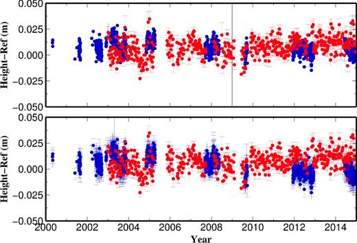
Time series of variation in height with respect to the mean value (Ref) for TGCV (blue) and SALB (red). TGCV series is represented with no estimation (bottom) and with estimation of an offset (top).

4.1.4 Canaries archipelago

GPS trends for the Canaries archipelago are represented in Fig. 10. Trends for stations in Lanzarote agree within their uncertainties. Trends for stations in Fuerteventura, excluding TARA, have not reached a good degree of robustness yet. There are no other terms of comparison for stations in the islands of Lanzarote, Fuerteventura and La Gomera. LPAL is the station with the longest record in La Palma, with all solutions presenting a subsidence trend, except JPL. JPL's trend for this station is 0.16 ± 0.58 mm yr⁻¹, while SOPAC's trend is −0.6 ± 0.3 mm yr⁻¹, in good agreement with the estimate by Saria et al. (2013) of −0.60 ± 0.23 mm yr⁻¹. All of these rates are lower than our solution (−1.16 ± 0.20 mm yr⁻¹). Our estimate for MAZO is not statistically different from that obtained for LPAL.

Figure 10.

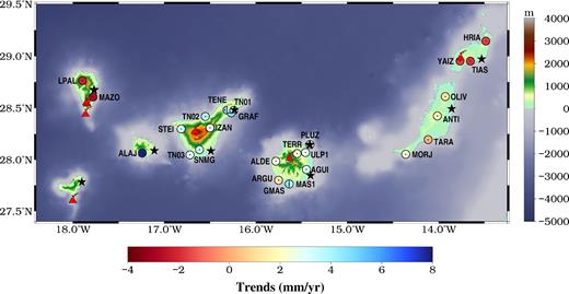
GPS trends (circles) and site locations for GPS and tide gauges (stars) in the Canaries archipelago. Also shown the locations of active central volcanoes (triangles).

Tenerife has several stations with long time series (IZAN, TN01, TN02 and TN03) yielding robust trends. The largest variations in trends are for the shorter series of SNMG, GRAF and STEI, but they seem to start converging with the trends presented by nearby stations with longer time series.

Most stations in Gran Canaria, with the exception of those with the longest records, have trends that suffered significant changes in the last years. The stations with the longest time series are MAS1, PLUZ and ULP1. Estimates for their trends are available in recent literature (see Table 4). Our estimates are in good agreement with those by Santamaría-Gómez et al. (2012). For GMAS we get essentially the same trend as Saria et al. (2013).

Table 4.

Trend estimates (in mm yr⁻¹) for GMAS, MAS1 and PLUZ (Gran Canaria).

	W2009a	R2013b	S2013c	SG2012d	SOPAC	JPL	This study
GMAS	–	–	0.03 ± 0.21	−0.35 ± 0.21	0.1 ± 0.3	−0.53 ± 0.63	0.07 ± 0.24
MAS1	−0.05 ± 0.27	−0.62 ± 0.04	−0.86 ± 0.19	−0.76 ± 0.24	−0.6 ± 0.1	−0.53 ± 0.33	−0.79 ± 0.13
PLUZ	−	−1.05 ± 0.06	−	−1.77 ± 0.17	–	–	−1.50 ± 0.24

a

^aWöppelmann et al. (2009).

^bRudenko et al. (2013).

^cSaria et al. (2013).

^dSantamaría-Gómez et al. (2012) (ULR6a solution).

The level of agreement between our solutions and those from the analysis centres used for comparison are summarized for the common GPS stations in Fig. 11.

Figure 11.

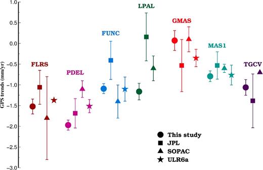
Comparison of GPS trends provided by different analysis centres for a set of common stations in the Macaronesian archipelago. Due to their high values, uncertainties for some solutions are not represented.

Despite the small number of common stations processed by the different analysis centres, the statistical analysis reveals no significant differences between them. For the seven common stations to JPL, SOPAC and our solutions, the 95 per cent confidence intervals for a null hypothesis of 0 mm yr⁻¹ mean using our solution as reference are 1.2 and 0.84 mm yr⁻¹, for JPL and SOPAC, respectively. The same confidence interval is slightly larger for the differences between JPL and SOPAC solutions (1.3 mm yr⁻¹). When considering the five stations also common to the ULR6a solution (and using this solution as reference), the confidence interval is again smaller in comparison with our solution (0.79 mm yr⁻¹) and similar in the comparison against JPL and SOPAC (0.91 and 0.90 mm yr⁻¹, respectively).

4.2 Glacial isostatic adjustment

GIA is partially responsible for changes in present-day GPS vertical trends. We compared GPS trends against the ICE-6G(VM5a) model (Argus et al.2014; Peltier et al.2015; Fig. 12). The present-day contribution of the GIA process is characterized by a subsidence rate ranging from ∼0.5 mm yr⁻¹ (for the Canary Islands) to more than 0.7 mm yr⁻¹ (Azores archipelago). Differences between GPS trends and ICE-6G(VM5a) predictions are less than 1 mm yr⁻¹ for ∼60 per cent of the stations. Differences for stations ARGU, TARA, TERC and PTRP are greater than 2 mm yr⁻¹. The correction of GPS trends with the ICE-6G(VM5a) yields a reduction of ∼40 per cent in the mean value, from about −1.4 to −0.85 mm yr⁻¹. Regionally, the best agreement between GPS trends and ICE-6G(VM5a) predictions is for the Madeira archipelago, with differences lower than ∼1 mm yr⁻¹ for all stations, and for Cape Verde station TGCV. For the majority of the stations in Macaronesia, the ICE-6G(VM5a) predictions underestimate the subsidence rate.

Figure 12.

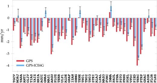
Differences (blue bars) between GPS trends (red bars) and GIA ICE-6G(VM5a) model predictions (black error bars represent GPS trend uncertainties).

These results indicate that the GIA process as dominant contribution to vertical land motion is far from being homogeneous for the Macaronesia and that other physical processes play a significant role, the most important likely being the tectono-volcanic deformation. In fact, islands in a dormant volcanic stage, such Madeira and Sal (Cape Verde), show a good agreement between GIA and GPS, whereas for those in tectono-volcanic active contexts the contribution of GIA is less relevant. One should note that GIA and other isostatic processes (such as the load of volcanic edifices) are continuous, slow acting processes while the tectono-volcanic deformation is related to more discreet events, occurring in time with shorter recurrence intervals. Thus, during periods of volcanic or tectonic unrest there should be disagreement between GPS trends and GIA predictions, while during inactivity periods GPS and GIA should concur.

Volcanic activity, tectonics and mass-wasting events play an important role in present-day vertical land motion in Macaronesia. The deformation connected to those events has, therefore, implications in establishing regional projections for mean sea level changes and consequently in deciding on mitigation actions. Assuming GIA as the dominant contribution to vertical land motion to correct tide gauge records in order to derive mean sea level may lead to significant deviations in those projections.

5 SEA LEVEL CHANGE

5.1 Tide gauges

The tide gauge data set for the Macaronesian islands is very heterogeneous both in terms of temporal range and completeness, resulting in a large diversity of trend estimates (Table 5). Many tide gauges in the Canary Islands, for example, are part of the recently established REDMAR Spanish network (Pérez et al. 2014) resulting in time series that are too short to derive reliable trend estimates (results for these series are presented just for the sake of completeness). Long time series but with large data gaps also need to be viewed with caution. In cases where more than one record is available for the same location (Flores, Funchal, Arrecife, Tenerife), we considered only the longer record.

Table 5.

Trends derived from tide gauge monthly series (⁠|${\dot{\rm U}_{\rm TG}}$|⁠, in mm yr⁻¹) and respective uncertainties (σ, in mm yr⁻¹). Also listed in this table, the nearest GPS site (NGL) and the approximate distance between the two locations (D, in km); otherwise, as Table 2. The TGs in the shaded rows are listed for the sake of completeness of this study.

SITE	Source	Location	λ	φ	Δt	CI	|${{{\bf \dot{U}}}_{{{\bf TG}}}}$|	σ	NGL	D
843	PSMSL	Santa Cruz das Flores (Flores)	− 31.117	39.450	33.3	58	2.28	0.86	FLRS	<1
2171	PSMSL	Lajes das Flores (Flores)	− 31.169	39.378	8.9	100	11.57	3.35	FLRS	9
258	PSMSL	Ponta Delgada (São Miguel)	− 25.671	37.736	36.5	72	3.52	0.42	PDEL	2
2024	PSMSL	Funchal II (Madeira)	− 16.913	32.644	11.1	92	3.95	1.82	FUNC	<1
218B	JASL	Funchal (Madeira)	− 16.907	32.642	27.6	96	3.07	0.57	FUNC	<1
2066	PSMSL	Arrecife 2 (Lanzarote)	− 13.530	28.972	6.7	97	− 0.12	3.59	TIAS	12
593	PSMSL	Arrecife (Lanzarote)	− 13.530	28.972	66.7	81	0.43	0.26	TIAS	12
2064	PSMSL	La Palma	− 17.768	28.678	7.8	86	3.37	3.69	MAZO	8
568	PSMSL	Santa Cruz B (La Palma)	− 17.769	28.672	18.9	86	− 1.10	1.13	MAZO	8
2048	PSMSL	Fuerteventura	− 13.858	28.493	10.9	95	2.65	1.77	OLIV	15
1803	PSMSL	Tenerife	− 16.233	28.483	22.3	95	5.14	0.85	TN01	1
565	PSMSL	Las Palmas C (Gran Canaria)	− 15.408	28.147	24.6	96	4.36	0.57	PLUZ	1
1802	PSMSL	Las Palmas D (Gran Canaria)	− 15.412	28.141	22.4	95	5.02	0.93	PLUZ	1
2065	PSMSL	La Gomera	− 17.108	28.088	7.8	96	8.52	3.85	ALAJ	13
2050	PSMSL	Granadilla (Tenerife)	− 16.490	28.085	8.4	96	6.54	2.35	SNMG	12
2049	PSMSL	Arinaga (Gran Canaria)	− 15.401	27.847	8.8	97	5.89	3.54	AGUI	8
2051	PSMSL	Hierro (El Hierro)	− 17.902	27.784	10.4	96	3.98	3.92	FRON	11
1914	PSMSL	Palmeira (Sal)	− 22.983	16.750	14.8	92	3.52	1.43	TGCV	<1

For the case of Flores, we have also tested a solution resulting from merging the records of Santa Cruz das Flores (PSMSL 843) and Lajes das Flores (PSMSL 2171), and introducing an offset to account for lack of levelling between both tide gauges. Despite the new series being a few years longer, we observed no significant change in trend and a small reduction in the uncertainty (estimated trend of 2.18 ± 0.70 mm yr⁻¹).

The analysis of the tide gauge data for Ponta Delgada has been studied by Ng et al. (2014), who obtained a trend of 2.5 ± 0.4 mm yr⁻¹ for the period 1978–2007, and a trend of 3.3 ± 1.5 mm yr⁻¹ for the period 1996–2007, in line with our estimate for the full time series. Ng et al. (2014) attributed the difference in trend for the two periods to a possible acceleration in the mean sea level.

For the Canaries archipelago and for the common tide gauges and similar time spans, our results are in very good agreement with those presented by Pérez-Gómez et al. (2015).

If we exclude the time series covering a time span of less than ∼15 yr (we consider these meaningless and are listed in Table 5 in shaded rows), relative sea level trends range from −1.1 mm yr⁻¹ at La Palma B to 5.1 mm yr⁻¹ at Tenerife. The threshold of ∼15 yr for deriving reliable long-term trends from tide gauge time series is still extremely optimistic, but the number of tide gauges in Macaronesia with time series long enough to fulfil the recommended requirements of 50–60 yr (e.g. Douglas 1991, 2001; Houston & Dean 2013) to remove decadal-scale fluctuations is very low.

5.2 Satellite altimetry

The trends for the SA grid points covering the Macaronesian region are presented in Fig. 13. They show a very consistent pattern for latitudes below ∼33°N, followed by a more disperse distribution for higher latitudes, associated with regional sea level variability and ocean dynamics.

Figure 13.

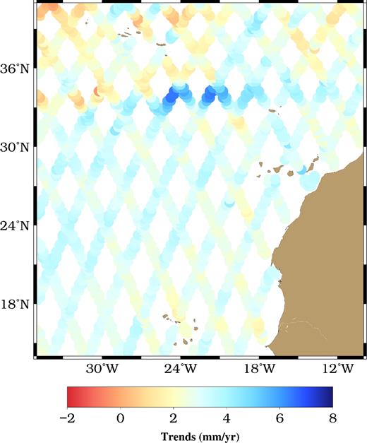
Satellite altimetry trends for the Macaronesian region.

In order to select the best representative SA grid point for comparison against TG corrected for GPS-derived vertical land movement, we tested three different approaches: (1) the closest grid point; (2) the best correlated grid point; (3) the average of all grid points within a degree of latitude and longitude of each tide gauge. The different approaches yield similar (and statistically not significant) results, but we elected the third option, in order to have a more robust estimate. The uncertainty for this average grid point was computed by error propagation of the uncertainties associated to each grid point estimate. The elected grid points are listed in Table 6, along with the closest TG and GPS locations. For the whole set of this averaged grids points, we obtain a mean value of absolute sea level of 3.0 ± 0.5 mm yr⁻¹ for Macaronesia.

Table 6.

Satellite altimetry trends (⁠|${\dot{\rm U}_{\rm SA}}$|⁠, in mm yr⁻¹) derived for a set of grid points (GP) and respective one-sigma uncertainties (σ, in mm yr⁻¹). All series span the same time interval (1993.0–2016.0). The table also lists the nearest tide gauge(s) (NTL, corresponding to the site ID listed in Table 5) and GPS (NGL) locations; otherwise, as Table 2.

GP	|${\dot{\rm U}_{\rm SA}}$|	σ	NTL	NGL
1	1.98	0.98	2171/843	FLRS
2	3.07	0.64	258	PDEL
3	3.15	0.58	218/2024	FUNC
4	2.79	0.58	2066/593	TIAS
5	2.80	0.49	2064/568	MAZO
6	3.62	0.55	2048	OLIV
7	3.14	0.50	1803	TN01
8	3.30	0.53	565/1802	PLUZ
9	3.29	0.52	2065	ALAJ
10	3.33	0.53	2050	SNMG
11	3.35	0.50	2049	AGUI
12	2.22	0.40	1914	TGCV

5.3 Combined observations

Sea level change in Macaronesia from tide gauges corrected for GPS-derived vertical land movement and satellite altimetry is displayed in Figs 14–17. These figures show also the SA grid points closest to each archipelago. Table 7 shows the trends resulting from the combination of tide gauges and GPS stations and the difference between the corrected tide gauge trends and satellite altimetry values, as well as the total uncertainty resulting from propagation of uncertainties for TG, GPS and SA. A limitation in this type of analysis results not only from the already mentioned shortness of TG time series, but also from the fact that the distance between the TG and some GPS stations exceeds largely an acceptable threshold to keep valid the assumption of absence of differential vertical land motion between them (Bevis et al.2002; Featherstone et al.2015). This limitation is particularly evident for São Miguel, where active tectono-volcanic are influencing vertical land motion for FRNS and VFDC. Other sources of breakdowns in that assumption for non-collocated TG and GPS can be of anthropogenic nature, such groundwater exploitation and reservoir storage, local subsidence (compaction and drainage) or uplift. In most cases, the contributions of these processes to vertical land motion are not suitably identified.

Figure 14.

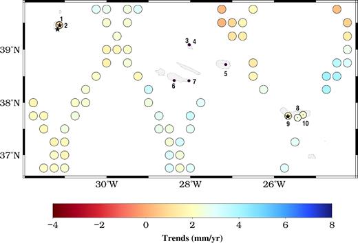
SA trends (large circles) and tide gauge corrected for GPS-derived vertical land motion (dotted smaller circles) for the archipelago of Azores. Numbers in the figure identify GPS stations listed in Table 2 and stars identity the location of tide gauges.

Figure 15.

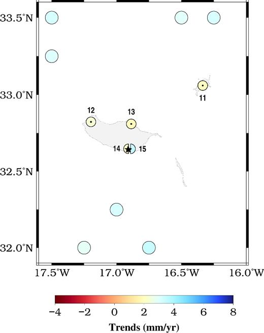
SA trends and tide gauge corrected for GPS-derived vertical land motion for the archipelago of Madeira. Otherwise, as in Fig. 14.

Figure 16.

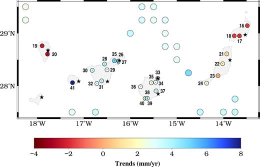
SA trends and tide gauge corrected for GPS-derived vertical land motion for the archipelago of Canaries. Otherwise, as in Fig. 14.

Figure 17.

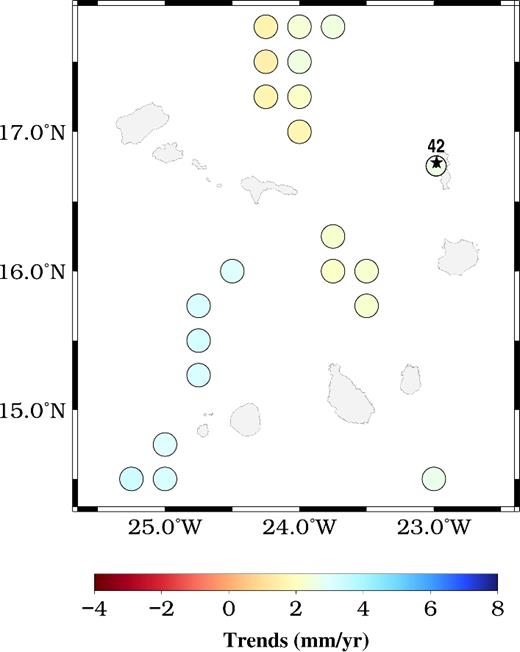
SA trends and tide gauge corrected for GPS-derived vertical land motion for the archipelago of Cape Verde. Otherwise, as in Fig. 14.

Table 7.

Trends (in mm yr⁻¹) from tide gauge (⁠|${\dot{\rm U}_{\rm TG}}$|⁠), GPS (⁠|${\dot{\rm U}_{\rm GPS}}$|⁠), combination of tide gauges and GPS stations (⁠|${\dot{\rm U}_{\rm C}}$|⁠), satellite altimetry (⁠|${\dot{\rm U}_{\rm SA}}$|⁠) time series, and difference between satellite altimetry trends and the corrected tide gauge (Δ), as well as the uncertainty (σ_Δ, in mm yr⁻¹) resulting from propagation of uncertainties for TG, GPS and SA.

TG	GPS	SA	|${\dot{\rm U}_{\rm TG}}$|	|${\dot{\rm U}_{\rm GPS}}$|	|${\dot{\rm U}_{\rm C}}$|	|${\dot{\rm U}_{\rm SA}}$|	Δ	σΔ
PS_843	FLOR	GP_01	2.28	− 1.55	0.73	1.98	1.25	1.39
PS_843	FLRS	GP_01	2.28	− 1.52	0.76	1.98	1.22	1.32
PS_258	FRNS	GP_02	3.52	− 1.36	2.16	3.07	0.91	0.82
PS_258	PDEL	GP_02	3.52	− 1.97	1.55	3.07	1.52	0.77
PS_258	VFDC	GP_02	3.52	− 0.96	2.56	3.07	0.52	0.84
UH_218B	PSTO	GP_03	3.07	− 1.12	1.95	3.15	1.20	0.76
UH_218B	PAUL	GP_03	3.07	− 0.74	2.33	3.15	0.82	0.75
UH_218B	STNA	GP_03	3.07	− 1.17	1.90	3.15	1.25	0.73
UH_218B	FUNC	GP_03	3.07	− 1.09	1.98	3.15	1.17	0.72
UH_218B	IMMA	GP_03	3.07	0.49	3.56	3.15	− 0.41	0.76
PS_593	HRIA	GP_04	0.43	− 2.08	− 1.65	2.79	4.44	0.42
PS_593	TIAS	GP_04	0.43	− 2.31	− 1.88	2.79	4.67	0.59
PS_593	YAIZ	GP_04	0.43	− 2.08	− 1.65	2.79	4.44	0.47
PS_568	LPAL	GP_05	− 1.10	− 1.16	− 2.26	2.80	5.06	1.27
PS_568	MAZO	GP_05	− 1.10	− 1.59	− 2.69	2.80	5.49	1.29
PS_2048	OLIV	GP_06	2.65	− 1.54	1.11	3.62	2.51	1.82
PS_2048	ANTI	GP_06	2.65	− 1.22	1.43	3.62	2.19	1.89
PS_2048	TARA	GP_06	2.65	− 2.54	0.11	3.62	3.51	1.82
PS_2048	MORJ	GP_06	2.65	− 0.30	2.35	3.62	1.27	1.84
PS_1803	TENE	GP_07	5.14	0.05	5.19	3.14	− 2.05	0.99
PS_1803	TN01	GP_07	5.14	− 0.80	4.34	3.14	− 1.20	0.98
PS_1803	GRAF	GP_07	5.14	− 0.22	4.92	3.14	− 1.78	1.10
PS_1803	TN02	GP_07	5.14	− 1.24	3.90	3.14	− 0.76	1.03
PS_1803	IZAN	GP_07	5.14	− 2.26	2.88	3.14	0.26	0.98
PS_1803	STEI	GP_07	5.14	− 1.61	3.53	3.14	− 0.39	1.07
PS_1803	SNMG	GP_07	5.14	− 1.49	3.65	3.14	− 0.51	0.99
PS_1803	TN03	GP_07	5.14	− 1.98	3.16	3.14	0.02	1.00
PS_565	PLUZ	GP_08	4.36	− 1.50	2.86	3.30	0.44	0.72
PS_565	ULP1	GP_08	4.36	− 1.52	2.84	3.30	0.46	0.72
PS_565	TERR	GP_08	4.36	− 1.98	2.38	3.30	0.92	0.72
PS_565	ALDE	GP_08	4.36	− 1.79	2.57	3.30	0.73	0.72
PS_565	AGUI	GP_08	4.36	− 1.06	3.30	3.30	0.00	0.76
PS_565	GMAS	GP_08	4.36	0.07	4.43	3.30	− 1.13	0.72
PS_565	MAS1	GP_08	4.36	− 0.79	3.57	3.30	− 0.27	0.69
PS_565	ARGU	GP_08	4.36	− 3.05	1.31	3.30	1.99	0.73
PS_1802	PLUZ	GP_08	5.02	− 1.50	3.52	3.30	− 0.22	1.03
PS_1802	ULP1	GP_08	5.02	− 1.52	3.50	3.30	− 0.20	1.03
PS_1802	TERR	GP_08	5.02	− 1.98	3.04	3.30	0.26	1.03
PS_1802	ALDE	GP_08	5.02	− 1.79	3.23	3.30	0.07	1.03
PS_1802	AGUI	GP_08	5.02	− 1.06	3.96	3.30	− 0.66	1.06
PS_1802	GMAS	GP_08	5.02	0.07	5.09	3.30	− 1.79	1.03
PS_1802	MAS1	GP_08	5.02	− 0.79	4.23	3.30	− 0.93	1.01
PS_1802	ARGU	GP_08	5.02	− 3.05	1.97	3.30	1.33	1.03
PS_2065	ALAJ	GP_09	8.52	− 0.67	7.85	3.29	− 4.56	3.89
PS_1914	TGCV	GP_12	3.52	− 1.06	2.57	2.22	− 0.35	1.50

The agreement between SA trends (⁠|${\dot{\rm U}_{\rm SA}}$|⁠) and TG trends corrected by GPS vertical land motion (⁠|${\dot{\rm U}_{\rm C}}$|⁠) varies substantially from island to island, being relatively consistent within each island.

For the Azores archipelago (Fig. 14), where TGs have long records and some GPS stations are close to the TG, we observe a discrepancy between |${\dot{\rm U}_{\rm C}}$| and |${\dot{\rm U}_{\rm SA}}$| exceeding 1 mm yr⁻¹ for Flores and PDEL (curiously the station with the longest GPS record and the less prone to the influence of tectono-volcanic processes). However, the uncertainties for these differences are close to the estimates.

For the Madeira archipelago (Fig. 15) we find a similar situation, where the combination the TG with the derived vertical land motion of FUNC (the most reliable and closest GPS station) is of 1.17 ± 0.22 mm yr⁻¹.

The level of concordance between |${\dot{\rm U}_{\rm SA}}$| and |${\dot{\rm U}_{\rm C}}$| for the Canaries archipelago (Fig. 16) is dissimilar for the different islands. For Lanzarote, TG time series is very long when compared to the remaining time series, resulting in a trend that does not reflect the more contemporary rates yielded by SA. On the other hand, GPS time series are not too long and they are too far (more than 10 km, in the best scenario) from the TG location to derive reliable vertical land motion. La Palma has a very peculiar situation, since TG presents a negative trend (nevertheless, within the uncertainty), which has no correspondence with an uplift at GPS stations, which are again distant from the TG location. The analysis for La Gomera and Lanzarote are affected by several hindering factors to derive any conclusions: very short time series for both TG and GPS and a significant distance between those locations, resulting in unrealistic trends that have no significance and are listed in Table 7 just for comprehensiveness purposes.

There is a fair agreement between |${\dot{\rm U}_{\rm SA}}$| and |${\dot{\rm U}_{\rm C}}$| for Tenerife and Gran Canaria, possibly due to the fact that the TG and SA time series cover a similar period of time. For Tenerife, the use of vertical land motion from four different sites yield differences smaller than 0.5 mm yr⁻¹ with respect to SA, despite the different periods of operation of GPS stations. Concerning Gran Canaria only when considering the vertical land motion estimated from two stations (GMAS and ARGU) we observed larger differences, with the remaining stations exhibiting differences smaller than ∼1 mm yr⁻¹, regardless of the TG used as reference (PS_565 or PS_1802). Those two GPS locations are far from the location of the TG.

There is also a good agreement between |${\dot{\rm U}_{\rm SA}}$| and |${\dot{\rm U}_{\rm C}}$| for Cape Verde (Sal, Fig. 17) that can also be due to the similarity of the time span covered by SA, TG and GPS time series, aided by the fact that TGCV is very close to the TG location.

For the TG trends corrected for GPS vertical land motion, the estimates vary from −2.7 mm yr⁻¹ (MAZO) to 5.2 mm yr⁻¹ (TENE) and there is, in general, a better agreement between |${\dot{\rm U}_{\rm C}}$| and |${\dot{\rm U}_{\rm SA}}$| than between |${\dot{\rm U}_{\rm TG}}$| and |${\dot{\rm U}_{\rm SA}}$|⁠. If we disregard the islands of La Palma, Lanzarote, and Fuerteventura, where very large disagreement between |${\dot{\rm U}_{\rm C}}$| and |${\dot{\rm U}_{\rm SA}}$| exist due to the identified limitations in the data, the average value of |${\dot{\rm U}_{\rm C}}$| is 3.0 ± 1.2 mm yr⁻¹ or 2.8 ± 1.2 mm yr⁻¹, depending on whether we use PS_1802 or PS_565 as reference TG for Gran Canaria.

6 CONCLUSIONS

The scientific relevance of understanding and quantifying sea level change in Macaronesia motivates a holistic assessment using all available instrumental records in the region, including a dense network of GPS continuous stations, tide gauges and satellite altimetry.

The analysis of GPS data for 42 stations in Macaronesia reveals that, with a few exceptions, GPS sites are experiencing subsidence, which is larger than the predictions of GIA model ICE-6G(VM5a), reinforcing the need for reliable vertical land motion estimates to correct tide gauge trends. Furthermore, due to their particular geodynamic setting, some stations suffer the influence of tectono-volcanic mechanisms, implying that special care must be taken into account when interpreting sea level variations from tide gauge measurements.

Relative sea level trends for a selected number of tide gauges in Macaronesia exhibit large dispersion, ranging from −1.1 mm yr⁻¹ at La Palma B to 5.1 mm yr⁻¹ at Tenerife. Sea level trends from tide gauge records corrected for vertical movement using the estimates from the GPS time series range from −2.7 mm yr⁻¹ to 5.2 mm yr⁻¹ and show generally a better agreement with satellite altimetry data than the uncorrected estimates. Absolute sea level trends from satellite altimetry average to 3.0 ± 0.5 mm yr⁻¹ for the Macaronesia area.

The agreement between satellite altimetry and tide gauge trends corrected for vertical land movement varies substantially from island to island, which can be mostly explained by the heterogeneity of the available time series in terms of length, temporal span and data gaps. The largest dissimilarity is found for Lanzarote and La Palma. For the remaining islands, there is a fair agreement, and ∼56 per cent of the trends derived from the combination of GPS and tide gauge observations differ by less than ∼1 mm yr⁻¹ with respect to the absolute sea level trends estimated from satellite altimetry for the last ∼23 yr, despite the heterogeneity in size of both GPS and tide gauge time series, and the influence of volcanic-tectonic processes affecting the position of some GPS stations.

Acknowledgments

We thank the editor and two anonymous reviewers for their constructive comments, which contributed to improve the manuscript.

We thank all the private and public institutions providing free access to GPS data, namely the International GNSS Service (http://igs.org), EUREF (http://www.epncb.oma.be), Canary GNSS Centre (http://www.canarygnsscenter.org), GRAFCAN (http://www.grafcan.es), IGN (http://www.ign.es), PGF (http://www.soest.hawaii.edu/pgf/), ReNEP (http://www.igeo.pt), REPRAA (http://www.repraa.azores.gov.pt), REPGRAM (http://www.repgram.org.pt), University of Las Palmas de Gran Canaria (http://www.ulpgc.es), and Faculdade de Ciências da Universidade de Lisboa (https://ciencias.ulisboa.pt). Tide gauge data were provided by the Permanent Service for Mean Sea Level (PSMSL) and the University of Hawaii Sea Level Center (UHSLC). Satellite altimetry data were provided by the DEOS’ Radar Altimeter Database System (RADS). Maps were created using Generic Mapping Tools (Wessel et al.2013). The HPC facilities operated by Instituto de Astrofísica e Ciências do Espaço (Universidade de Lisboa) are gratefully acknowledged. The authors wish to acknowledge FCT (Fundação para a Ciência e a Tecnologia) projects UID/EEA/50014/2013 and IF2013. This publication is supported by FCT project UID/GEO/50019/2013 - Instituto Dom Luiz.