Joint inversion estimate of regional glacial isostatic adjustment in Antarctica considering a lateral varying Earth structure (ESA STSE Project REGINA)

Summary

A major uncertainty in determining the mass balance of the Antarctic ice sheet from measurements of satellite gravimetry, and to a lesser extent satellite altimetry, is the poorly known correction for the ongoing deformation of the solid Earth caused by glacial isostatic adjustment (GIA). Although much progress has been made in consistently modeling the ice-sheet evolution throughout the last glacial cycle, as well as the induced bedrock deformation caused by these load changes, forward models of GIA remain ambiguous due to the lack of observational constraints on the ice sheet's past extent and thickness and mantle rheology beneath the continent. As an alternative to forward-modeling GIA, we estimate GIA from multiple space-geodetic observations: Gravity Recovery and Climate Experiment (GRACE), Envisat/ICESat and Global Positioning System (GPS). Making use of the different sensitivities of the respective satellite observations to current and past surface-mass (ice mass) change and solid Earth processes, we estimate GIA based on viscoelastic response functions to disc load forcing. We calculate and distribute the viscoelastic response functions according to estimates of the variability of lithosphere thickness and mantle viscosity in Antarctica. We compare our GIA estimate with published GIA corrections and evaluate its impact in determining the ice-mass balance in Antarctica from GRACE and satellite altimetry. Particular focus is applied to the Amundsen Sea Sector in West Antarctica, where uplift rates of several centimetres per year have been measured by GPS. We show that most of this uplift is caused by the rapid viscoelastic response to recent ice-load changes, enabled by the presence of a low-viscosity upper mantle in West Antarctica. This paper presents the second and final contributions summarizing the work carried out within a European Space Agency funded study, REGINA (www.regina-science.eu).

Glaciology, Global change from geodesy, Gravity anomalies and Earth structure, Loading of the Earth, Antarctica, Joint inversion

1 INTRODUCTION

The largest uncertainty in mass balance estimates for the Antarctic ice sheet (AIS) from gravimetric techniques is caused by the poorly known viscoelastic deformation of the solid Earth in response to past changes in glacial loads (e.g. Shepherd et al. 2012, suppl.). The mass movement in the Earth's interior associated with this glacial isostatic adjustment (GIA) causes an apparent mass change, which has to be separated and removed from the Gravity Recovery and Climate Experiment (GRACE) signal of present ice-mass change using a GIA estimate. The total magnitude of this correction for Antarctica lies between 50 and 200 Gt yr⁻¹ depending on the model assumptions (Martín-Español et al.2016b), and is comparable in magnitude to the ice-dynamic imbalance observed today (e.g. Rignot et al.2011b). The rates of bedrock uplift associated with GIA are typically below 1 cm yr⁻¹, and are considerably smaller than the typical range of ice elevation rates ranging from decimetres to metres per year measured with satellite altimetry. Nevertheless, when integrated over the entire ice sheet, GIA causes a systematic bias in the altimetry data, which has to be corrected. In contrast, vertical deformations of the Earth surface measured by the global navigation satellite systems are significantly affected by GIA (e.g. Thomas et al.2011).

Two principal approaches exist for estimating GIA. First, forward-modeling GIA by forcing a viscoelastic Earth model with an ice-loading history (Wu & Peltier 1982; Nakada & Lambeck 1988; Peltier 1994; Kaufmann 2002; Peltier 2004), which can either be based on a numerical ice-sheet model responding to climate forcing (Whitehouse et al.2012), or reconstructed from geomorphological observations of ice thickness (Ivins & James 2005). A combination of both reconstruction methods is also possible (e.g. Tarasov et al.2012). This approach is henceforth called GIA forward modeling. Second, it is possible to estimate GIA from multiple geodetic measurements with different sensitivities to GIA and present-day ice-mass change processes (Wahr et al.2000; Velicogna & Wahr 2002; Riva et al. 2009; Wu et al.2010; Gunter et al.2014; Martín-Español et al.2016a)—henceforth called GIA inversion estimate. Although much progress has been achieved in numerical modeling of the coupled ice/solid Earth system (e.g. Gomez et al.2013; Konrad et al.2015), as well as in the coverage of Global Positioning System (GPS) data (Bevis et al.2009) and interpretation of the long-term trends in the satellite data, large differences remain between the various GIA solutions, causing substantial uncertainty in GRACE ice-mass balances for Antarctica (Martín-Español 2016b).

In this study, we derive a new empirical GIA estimate for Antarctica by the inversion of multiple space-geodetic observations. We advance this approach, compared to previous efforts (e.g. Gunter et al.2014), through a reassessment of the input data sets (REGINA paper I—Sasgen et al.2017), including an updated and augmented data set of GPS uplift rates, and by basing the joint inversion on local viscoelastic response functions, allowing us to account for known lateral variations in the Earth structure of Antarctica. Our approach, based on viscoelastic response functions, is also different from the Bayesian estimation scheme presented in Martín-Español et al. (2016a), and allows us to address, in particular, the large uplift rates presumably enabled by low upper-mantle viscosities in West Antarctica.

As was done in a more recent study (Martín-Español et al.2016a), we include GPS uplift rates in addition to GRACE and altimetry data. This allows us to reduce the influence of the a priori snow/ice density distribution which is necessary to convert elevation changes to mass changes. In addition, we refine the assumption of an average rock density, transitioning from shelf to continental areas, applied in the work of Riva et al. (2009) and Gunter et al. (2014) for converting GIA-induced geoid-height rate to radial displacement rate. Unlike some other studies, we do not pre-define regional spatial patterns (Sasgen et al.2013) or length scales (Martín-Español et al.2016a) of the expected GIA signal. Instead, to account for the dynamics of the GIA process, we base our combination on viscoelastic response functions to a disc load forcing for an ensemble of Earth structures, representing the laterally heterogeneous lithosphere thickness and mantle viscosity in Antarctica (e.g. Morelli & Danesi 2004).

This paper first presents the combination method we have developed and applied, then summarizes the preparation of the input data sets and the viscoelastic response functions, which are described in detail in REGINA paper I (Sasgen et al.2017). Finally, we discuss the GIA estimate and its impact on GRACE and altimetry measurements derived mass and volume balances, and compares the estimates to previously published GIA corrections.

2 METHOD

2.1 Formulation of problem

The separation of present-day ice-mass change and GIA is enabled by the different sensitivities of the satellite observations with respect to present and past load changes (Fig. 1). In the following, m_pd, denotes present-day mass changes of the ice sheet, as the net balance of snow accumulation, ablation and ice-dynamic flow, while m_past denotes mass changes of the ice sheet that occurred in the past (before our observation period) and cause GIA. The parameter h_c denotes changes in the firn air content caused by firn compaction (see Ligtenberg et al.2014). Firn compaction decreases the firn air content (with no mass change), lowering the surface elevation (and thus volume) of the ice sheet, but it has no effect on gravity or bedrock elevation. Here, the rate of firn compaction is subtracted from the elevation rates from altimetry as the final processing step of the altimetry data set. More details are provided in REGINA paper I (Sasgen et al.2017). In contrast, snow accumulation is considered by the spatial distribution of the mean surface density obtained from RACMO2/ANT. The spatial distribution of regions of snow accumulation and regions dominated by ice dynamics constitutes our snow/ice density mask, ρ used to relate altimetry and gravimetry signals (see Section 3.4.1).

Figure 1.

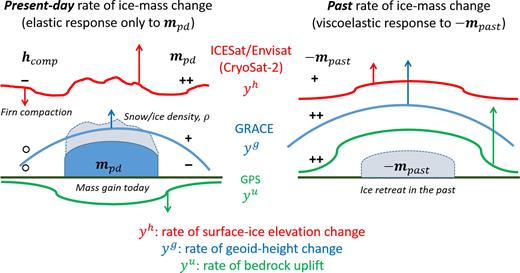
Concept of separating present-day rates of ice-mass change, m_pd, and past rates of ice-mass change, m_past, inducing GIA. Shown are the sign and sensitivity of the rate of elevation change, rate of gravity-field change and rate of bedrock displacement, y^h, y^g and y^u, respectively, to changes in m_pd and m_past, as well as to the rate of firn compaction, h_comp. Sensitivities are indicated as ++ high positive, + positive, − negative and ° no sensitivity.

Since the GIA signal, the target of this study, occurs at an approximately constant rate over the time span of the satellite observations, we restrict ourselves to considering linear rates of change. That is, the parameters m_pd, m_past and h_comp denote linear rates of change. Likewise, the observations from altimetry, gravimetry and GPS are incorporated in terms of linear rates of change, adjusted to the original observation time-series. Details of the determination of the optimal linear trends for each data set are described in REGINA paper I (Sasgen et al.2017).

The considered observations are rate of geoid-height change, y^g, rate of bedrock uplift, y^u, and rate of surface-ice elevation change, y^h. With the conceptual separation of m_pd, m_past and h_comp the observation equations can be arranged in the following system of linear equations:

\begin{equation}\left( {\begin{array}{c} {{y^g}} \\ {{y^u}}\\ {{y^h}} \end{array}} \right) = \left( {\begin{array}{c{@}{\quad}c{@}{\quad}c} {{F_e}}&{{F_v}}&0 \\ {{G_e}}&{{G_v}}&0 \\ {{H_e}}&{{G_v}}&{{E_w}} \end{array}} \right)\left( {\begin{array}{c} {{m_{{\rm{pd}}}}} \\ {{m_{{\rm{past}}}}}\\ {{h_{{\rm{comp}}}}} \end{array}} \right),\end{equation}

(1)

where F_e|v represents the elastic | viscoelastic response functions for the rate of geoid-height change, G_e|v represents the elastic | viscoelastic response function for the rate of bedrock uplift, E_w stands for the (filtered) equivalent water-height change. The response function H_e = E_w/ρ  + G_e for the elevation change (here, ice-sheet topography) is obtained by applying the snow/ice density distribution (Section 3.4.1) and correcting for associated elastic surface deformation (E_w ≫ ρG_e). The viscoelastic response functions F_v and G_v depend on the timing of the load change and the Earth model parameters, such as the thickness of the elastic lithosphere and the mantle viscosity structure. For a fixed temporal evolution of the load and a specific set of Earth model parameters, the elastic and viscoelastic responses are linear functions of the magnitude of the load, m_past. This is a consequence of the linearized theory of a Maxwell-viscoelastic continuum adopted here. The elastic response functions F_e and G_e are based on the Preliminary Reference Earth Model (Dziewonski & Anderson 1981). For details on the generation of the viscoelastic response functions, see REGINA paper I (Sasgen et al.2017).

The aim is to determine the unknown variables m_pd, m_past and h_comp, based on the observations y^g, y^u and y^h. The system of equations can be solved for the three unknowns at locations where all three data types are available. However, as described later, the problem is ill-posed requiring regularization to stabilize the inversion, which is further complicated as F_e|v and G_e|v are of different spatial smoothness. Here, we apply a Tikhonov L₂ regularization (e.g. Tikhonov & Arsenin 1977), providing smooth solution vectors, m_pd, m_past and h_comp; the optimal regularization parameter λ is determined based on the misfit between observed and predicted measurements, |$\|{y^u} - {\hat{y}^u}\| + \|{y^g} - {\hat{y}^g}\|$| (see Supporting Information, SI). In addition, to overcome the limitations of the spatial coverage of the GPS data, the combination follows a two-step approach. First, gravity and altimetry trends are combined assuming the elevation rates are purely caused by present mass changes, m_pd. In a second step, GPS uplift rates, clustered according to the spatial GRACE resolution, are included to provide a correction on the estimate of m_pd, which is then updated in an iterative procedure. The scheme of the iterative procedure is shown in Fig. 2.

Figure 2.

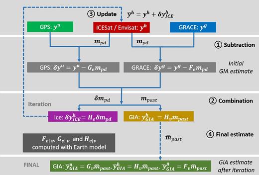
Scheme for combining GRACE, Envisat/ICESat and GPS data. Step 1 involves producing a first-order GIA estimate based on subtracting present-day ice-mass change inferred from altimetry from the GRACE gravity field trends. In Step 2, GPS uplift rates (corrected for the elastic effect based on altimetry) are used to separate residual present-day ice-mass change from GIA; the residual present-day ice-mass change is then used to locally improve altimetry field describing present-day ice-mass change.

Figure 3.

Envisat/ICESat rate of elevation change for 2003–2009 (m yr⁻¹). Data are corrected for the rate of firn compaction, h_comp, based on firn compaction module of RACMO2/ANT (Ligtenberg et al.2011). Effects from snow accumulation are not removed. For details see REGINA paper I (Sasgen et al.2017).

The estimates are performed on a geodesic grid (ICON 1.2 grid, status year 2007) used for the Max-Planck-Institute general circulation model (e.g. Wan et al.2013); grid cells are represented by circular discs of averaged equal area corresponding to a radius of 63 ± 1 km. The signals for the Antarctic continent are obtained by rotating the axisymmetric load and response functions to the coordinates of the geodesic grid, and subsequent superposition. The distribution of discs (total number: 1175) is limited to the areas confined by present-day grounding line and shelf outlines of Antarctica (continent: 1022 discs; ice shelves: 153 discs; see SI).

2.2 Step 1: combination of GRACE and Envisat/ICESat

First, we combine y^g and y^h, for the time period 2003–2009, similar to the approach presented in Gunter et al. (2014). For this, we correct the ice elevation changes for firn compaction h_comp using output of the firn compaction model of Ligtenberg et al. (2011). The remaining ice elevation changes are assumed to be related to snow and ice thickness changes of varying density. This reduces eq. (1) to

\begin{equation}\left( {\begin{array} {c} {{y^g}} \\ {{y^h}} \end{array}} \right) = \left( {\begin{array}{c{@}{\quad}c} {{F_e}}&{{F_v}}\\ {{H_e}}&{{G_v}} \end{array}} \right)\left( {\begin{array}{@{}*{1}{c}@{}} {{m_{{\rm{pd}}}}}\\ {{m_{{\rm{past}}}}} \end{array}} \right).\end{equation}

(2)

Furthermore, in this first step, viscoelastic deformation underlying the altimetry measurement is neglected, such that G_v = 0, as rates of ice elevation changes driven by surface processes are on the order of tens to hundreds of millimetres per year, while the GPS-measured uplift rates are typically at the level of a few millimetres per year, even though they can reach up to 30 mm yr⁻¹ in the Amundsen Sea Embayment (e.g. Groh et al.2012). With these assumptions, m_pd can directly be estimated from y^h = H_em_pd. The gravity field change caused by GIA to past load changes then becomes

\begin{equation}{F_v}{m_{{\rm{past}}}} = {y^g}{\rm{\ }} - \left( {{F_e}{m_{{\rm{pd}}}}} \right),\end{equation}

(3)

which is then solved for m_past in a least-squares sense with Tikhonov regularization. This is considered as our first-order GIA estimate and similar to the solution presented in eq. (1) of Gunter et al. (2014). It relies on the assumptions that firn compaction has successfully been removed from the altimetry data and that the a priori snow/ice density mask is correct.

Similarly, the GPS rates are corrected for elastic deformation based on the mass changes inferred from altimetry y^u − (G_em_pd). It should be noted that instead of applying m_pd to elastic response functions in Step 1, high-resolution uplift rates are calculated from the altimetry field using the density mask and surface load Love numbers (spherical-harmonic cut-off degree 512). The difference between both approaches is, however, minor for most GPS sites and has a negligible impact on the final GIA estimate.

2.3 Step 2: including GPS rates

Similarly, to the gravity field trends in Step 1, the GPS rates are corrected for elastic deformation based on the mass changes inferred from altimetry y^u − (G_em_pd). It should be noted that instead of applying m_pd to elastic response functions in Step 1, high-resolution uplift rates are calculated from the altimetry field using the density mask and surface load Love numbers (spherical-harmonic cut-off degree 512 and corresponding spatial half-wavelength of ca. 40 km). The difference between both approaches is, however, minor for most GPS sites and has a negligible impact on the final GIA estimate.

Next, to improve the first-order GIA estimate obtained in Step 1, residual present-day ice-mass changes are identified by including GPS uplift rates in this step as follows. Let δy^g = y^g  − F_em_pd and δy^u = y^u  − G_em_pd be the residual GRACE and GPS trends after subtracting the first-order estimates of present-day mass changes, m_pd. The δm_pd, previously unaccounted for, may arise from poor coverage in the altimetry data, an incorrect snow/ice density mask, or an inadequate correction for firn compaction. Then, an update of the present-day mass change, δm_pd and the past mass change, m_past, can be estimated by solving the reduced system of linear equations,

\begin{equation}\left( {\begin{array}{c} {\delta {y^g}}\\ {\delta {y^u}} \end{array}} \right) = \left( {\begin{array}{c{@}{\quad}c} {{F_e}}&{{F_v}}\\ {{G_e}}&{{G_v}} \end{array}} \right)\left( {\begin{array}{@{}*{1}{c}@{}} {\delta {m_{{\rm{pd}}}}}\\ {{m_{{\rm{past}}}}} \end{array}} \right).\end{equation}

(4)

Here, the complementarity of the response functions with respect to present-day and past mass changes is of advantage. For example, a measured signal with positive uplift and negative gravity field change will be, at least in parts, caused by present-day ice-mass changes and the associated elastic response. Eq. (4) allows estimating this remaining present-day ice-mass change and updating the GIA estimation accordingly.

Due to the sparse distribution of the GPS data, and to avoid an underdetermined system of equations, it is necessary to reduce the observation and solution domain to the k_max grid locations (here, k_max =  42) closest to the GPS or mean GPS site positions of the clustered data (see Section 3.2), respectively, |$\delta {y^{g|u}} = {\rm{\ }}\{ {y_k^{g|u}} \}$| and |$\delta m_{{\rm{pd\ }}|{\rm{\ past}}}^k = {\rm{\ }}\{ {m_{{\rm{pd\ }}|{\rm{\ past}}}^k} \}$|⁠, for k =  1, 2, …, k_max. Note that the corrections |$m_{{\rm{pd\ }}|{\rm{\ past}}}^k$| determined at the GPS locations, affect the solution only in an area governed by spatial wavelength of the respective response function.

Next, we update the first-order estimate of the surface-ice elevation change from altimetry based on the residual present-day ice-mass change we estimated with eq. (4), according to |${\hat{y}^h} = {y^h}{\rm{\ }} + {\rm{\ }}\delta y_{{\rm{ICE}}}^h = {y^h} + {H_e}\ \delta {m_{{\rm{pd}}}}$|⁠. Note that here H_e is a matrix of dimension k_max × i_max relating the mass change at the GPS location k to elevation rate of each disc on the geodesic grid, i.

We now replace y^h with |${\hat{y}^h}$| (update the present-day ice-mass change estimate of the previous step) and repeat Steps 1 and 2 until the updates of |$\delta y_{{\rm{ICE}}}^h$| are negligible, which is achieved after about three iterations in our final GIA estimate, |$\hat{y}_{{\rm{GIA}}}^g = {F_v}{\hat{m}_{{\rm{past}}}}$|⁠, and |$\hat{y}_{{\rm{GIA}}}^{u|h} = {G_v}{\hat{m}_{{\rm{past}}}}$|⁠, where the |${\hat{m}_{{\rm{past}}}}$| refers to the final past mass change estimate.

3 INPUT DATA SETS

3.1 Altimetry

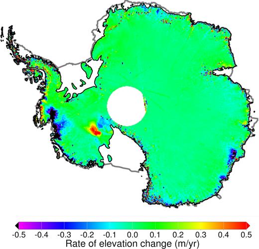
Rates of elevation change y^h of the ice sheet are obtained from laser and radar altimeters of ICESat and Envisat, respectively, for the coeval time interval 2003 February to 2009 October. We use both data sets to improve the spatial and temporal coverage afforded by their combination. To test the stationarity of the recovered GIA estimate, we extend the time-series up to 2013 December by including CryoSat-2 rates of elevation change for the years 2010–2013 (Helm et al.2014). We also use the prolonged time-series of the altimetry data sets to assess the impact of our GIA estimate on volume balance estimates. Details on the processing of the altimetry data sets are provided in REGINA paper I (Sasgen et al.2017).

We determine ICESat elevation rates y^h based on release 33/633 data from 2003 February until 2009 October (Abshire et al.2005). To estimate elevation change rates, we use multivariate regression to fit rectangular planes to near repeat tracks of ICESat measurements (Howat et al.2008) from which topographic slope (both across and along tracks) and y^h are simultaneously estimated.

For Envisat radar altimetry, time-series of height changes are provided by Flament & Rémy (2012), based on an along-track approach. Elevation trends were estimated every 1 km along track, by binning all the echoes within a 500 m radius and then fitting a 10-parameter least-squares model in order to correct for the across-track topography and changes in snowpack properties (Flament & Rémy 2012).

Elevation changes from both ICESat and Envisat data were gridded into a 10 × 10 km grid on a polar-stereographic projection (central latitude 71°S; central longitude 0°W and origin at the South Pole). To increase the coverage and reliability of the y^h estimate, we produce a combination of elevation rates based on both data sets. For each grid cell, the elevation rate was estimated from the data set with the smaller standard error. In this way, elevation rates over areas with steep topography and along the ice-sheet margins were mainly derived from ICESat, while Envisat was chosen over some flat areas and regions where ICESat data were not present (see fig. 1.1 from Sasgen et al.2017). After the combination, we apply a correction for the rate of firn densification obtained from the firn deification model of Ligtenberg et al. (2011), driven by RACMO2/ANT.

3.2 GPS uplift rates and clustering algorithm

The GPS processing strategy is similar to that of Thomas et al. (2011), but with more recent processing software (GIPSY-OASIS 6.2) and background model updates included, and covering the time interval 1995.0–2013.7. A mini ensemble of processing runs was also performed to improve understanding of potential systematic processing errors. The processing strategy and ensemble, as well as the rate estimation are described in full detail elsewhere (see Sasgen et al. 2017). Rates are in ITRF2008, which is defined to realize zero translations and translation rates with respect to the mean Earth centre of mass (Altamimi et al.2011). A summary of the processing strategy on uplift rates, and comparisons with uplift rates from earlier studies are given in REGINA paper I (Sasgen et al.2017). Note that we do not correct for Antarctic bedrock displacement related to co- and post-seismic deformation following large earthquakes, for example, intraplate Earthquake of 1998 with a magnitude of ∼8.2 (Nettles et al.1999; King & Santamaría-Gómez 2016). The potential influence on our GIA estimate is discussed in Section 4.1.

We now build regional clusters of the estimated uplift rates at the 118 Antarctic GPS sites. The rationale for this is the observation that neighbouring sites with discrepant uplift rates often have large formal errors because the rates are based on campaign data or short measurement time spans. In addition, the GIA signature is expected to have a regional characteristic. Differences between observed uplift rates of accurate sites in close proximity may be caused by (small) changes in elastic accumulation or local tectonics, that is, geophysical noise, not by local variability in GIA. Because we perform the joint inversion on a grid with node distances of ca. 120 km, and GRACE and filtered altimetry input data sets with a spatial resolution of about 200 km (half-wavelength), we have no need for individual uplift rate estimates for sites separated by only a few tens of kilometres. Instead, we consider a weighted average of nearby sites to be more robust.

The clustering algorithm operates as follows; for each threshold distance in turn (here: 10, 20, 50, 100, 150, 200 and 220 km), independent pairs of sites/clusters closer to each other than this threshold distance are merged by calculating the weighted mean of their uplift rates, and the simple mean of the site/cluster positions. The procedure is repeated until no new pairs created by these mergers are found within the threshold, and then the threshold is increased and iteration is restarted. Fig. 4 shows the results of the clustering with 200 km maximum threshold, which is the preferred choice for the joint inversion, considering the GRACE resolution (spatial half-wavelength of 200 km). It is evident that the main regional characteristics of the uplift rates recovered with GPS are retained, while discrepant sites at the same or nearby locations are merged, considering their respective uncertainties, to a representative average. The similar smoothness of the deformation field from GPS and the GRACE gravity field avoids the occurrence of artefacts in the inversion. The number of clusters with the 200 km maximum threshold is 42 (from individual 118 sites). Note that the clustering is carried out on the initial data set, representing elastic and viscoelastic uplift rates.

Figure 4.

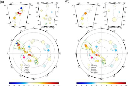
Uplift rates in Antarctica, for (a) 108 available GPS sites, and (b) 42 clusters after application of the clustering algorithm with a threshold distance of 200 km. Symbol colour denotes uplift rate (mm yr⁻¹) and symbol area denotes 1σ confidence limit

3.3 Gravimetry

We calculate the linear trend of the gravity field over Antarctica, expressed apparent water column of surface-mass change, y^g, by adjusting a multiparameter model (constant, linear trend, annual and semi-annual harmonic amplitudes) within the time period 2003 February to 2009 October (coeval to Envisat/ICESat measurement period). This time-series is derived from monthly Stokes coefficients from GRACE, up to degree and order 50 corresponding to a spatial half-wavelength of 200 km, provided by the Center for Space Research (CSR; Bettadpur 2012), release 5. Consistent with the GPS processing, the GRACE reference frame is ITRF2008. We reduce the typical north–south correlated error structures in GRACE monthly solutions by adapting the de-striping filter of Swenson & Wahr (2006, Swenson filter) to the region of Antarctica. Chambers & Bonin (2012) have previously performed a similar filter enhancement for global oceanic signals. We optimize the trade-off between (i) the signal corruption of synthetic data, and (ii) the effectivity of the noise reduction, inferred by filtering the residual GRACE minus altimetry trends south of 60°S. This residual is considered an upper bound for the uncertainty of the GRACE uncertainty. The optimal values for the Swenson filter minimize the quadratic sum of signal corruption and residual noise. For details see REGINA paper I (Sasgen et al.2017).

In a second step, to increase the robustness of the temporal linear trends, non-linear (de-trended) surface-mass variations associated with snow accumulation events are reduced from the GRACE monthly solutions. For this purpose, we convert the surface-mass balance (SMB) of the regional atmosphere and climate model RACMO2/ANT (Lenaerts et al.2012) into monthly sets of spherical-harmonic coefficients representing the storage changes of the ice sheet. After de-correlation with the optimized Swenson filter and the reduction of the non-linear mass components, the remaining noise is suppressed with a Gaussian filter of 200 km, which is estimated as the optimal half-width by applying the Wiener optimal filter (Sasgen et al.2006). Since the quality of GRACE monthly solutions varies over time, for example, due to evolving orbital sampling patterns, information on time-dependent error levels is introduced by month-dependent weighting in the estimation of the linear trends (e.g. Rangelova & Sideris 2008). Formal uncertainties of the trend are estimated based on the residual signal (after the multiparameter adjustment). This error estimate does not account for serial correlation of the residuals. Williams et al. (2014) report that such serial correlation increases the uncertainty of trends by factors typically on the order of 2, but sometimes reaching 6. The resulting linear trend, as well as the altimetry data filtered similar to GRACE is shown in Fig. 5.

Figure 5.

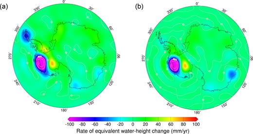
Rate of surface-mass change for the time period 2003–2009 from (a) GRACE (CSR release 05) with the optimized Swenson & Wahr (2006) and 200 km Gaussian filtering and (b) Envisat/ICESat applying the snow/ice density distribution shown in Fig. 3 and filtering similar to the GRACE trends (Gaussian filter of 200 km half-width). The spherical-harmonic cut-off degree and order is 50. The surface-mass change is expressed as millimetre water-equivalent (mm w.e.) yr⁻¹.

Based on comparing signals over the continent and the ocean, Williams et al. (2014) suggest that a large part of the serial correlation is due to actual ice-mass variability and not caused by errors of the GRACE observing system. To reduce such autocorrelation of residuals, we subtract modeled surface-mass balance (SMB) fluctuation effects prior to estimating the trends, leading to a smaller residual and, hence, smaller empirical uncertainties of the trend. More details are found in Sasgen et al. (2017), even though a thorough investigation on the effectiveness of the SMB to reduce residual autocorrelation is yet to be undertaken. Nonetheless, in the actual inversion procedure (Section 2), we adopt an uncertainty estimate that is more pessimistic: we chose the deviations between trends from different GRACE release, which are typically larger than the uncertainties derived for a single release.

3.4 Auxiliary data

3.4.1 Snow/ice density estimate

We use a snow/ice density distribution (Fig. 6) for converting the elevation rates derived from Envisat/ICESat altimetry to surface-mass rates during Step 1 of the GIA estimate. Similar to the procedure applied in Riva et al. (2009), the snow/ice density mask is constructed as follows: elevation changes within regions with surface-ice velocities >100 m yr⁻¹ or surface-elevation rates |y^h| > 0.3 m yr⁻¹ are assigned the density of ice, while for the remaining regions the mean surface density is obtained from RACMO2/ANT for the time period 1979–2010 (Lenaerts et al. 2012). The surface-ice velocity field is a combination of InSAR velocities (Rignot et al.2011a) and balance velocities (Bamber et al.2000). The temporal coverage of the InSAR product is 1996–2011 (https://nsidc.org/data/docs/measures/nsidc0484_rignot/, last accessed 22 September 2017).

Figure 6.

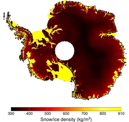
Snow/ice density distribution applied to the rates of elevation change from altimetry, during Step 1 of the GIA estimation.

The construction of our density mask follows the rationale that high, localized elevation rates are typically associated with fast glacier flow or strong glacier thinning and retreat, while broader patterns of moderate elevation change are dominantly driven accumulation variations. The additional threshold criterion attributing to |y^h| > 0.3 m yr⁻¹, the density of ice accounts to some extent for ice-dynamic thinning that has occurred since the surface-ice velocities have been measured (1996–2011; Rignot et al.2011a). An exception is made for the Kamb Ice Stream (Ice stream C), where dynamic elevation changes are known to occur in spite of low velocities (Retzlaff & Bentley 1993). It should be emphasized that we refrain from additionally correcting for anomalies in the surface-mass balance due to the rather short meteorological measurement records underlying RACMO2/ANT (1978–2015) and the associated problem of defining a reference climatology for Antarctica.

3.4.2 Earth structure and distribution of viscoelastic response functions

In Antarctica, properties of the Earth's lithosphere and mantle are considered to vary strongly between East and West Antarctica; while the East AIS rests on a cratonic structure, West Antarctica is dominated by a rift system. Seismic shear wave velocity anomalies support this geological inference (Morelli & Danesi 2004), indicating a much thinner elastic lithosphere, h_L, and lower upper-mantle viscosities in West Antarctica compared to East Antarctica. Here, we accommodate the rheological differences between East and West Antarctica by selecting from our ensemble of Earth structures (see REGINA paper I, Sasgen et al.2017), those viscoelastic response functions that match the Earth structure model by Priestley & McKenzie (2013). In particular, we derive the thickness of the elastic lithosphere from the 3-D distribution of mantle viscosities provided by Priestley & McKenzie (2013), by assuming that lithosphere and mantle layers with viscosities >10²² Pa s respond elastically on the considered timescale of a few millennia. The resulting thickness of the elastic lithosphere ranges from 30 km in parts of the Antarctic Peninsula, to 200 km in East Antarctica, which is a plausible range considering similar geological regimes. Similar lithosphere thickness values (±10 km) are obtained by applying thresholds of 10²¹ Pa s (h_L thicker) to 10²³ Pa s (h_L thinner); however, the preferred threshold leading to the GIA estimate best fitting the data is 10²² Pa s (see Section S.4, SI). In equilibrium state between load forcing and deformational response, the viscoelastic response function is only governed by the thickness of the elastic lithosphere. Therefore, currently mantle viscosities are neglected in the selection of the response functions. Note, for consistency with the satellite data realized in the International Terrestrial Reference Frame (ITRF) reference frame, the response functions are calculated in the centre of mass. Although the assumption of an equilibrium state clearly does not capture the full-dynamic behaviour of GIA, we consider it a good approximation for the low-viscosity regime of West Antarctica and necessary to avoid an additional a priori information on the temporal evolution of the ice sheet. In contrast, the cratonic structure underneath East Antarctica suggests higher mantle viscosities and, therefore, longer relaxation times, particularly in the central part of the ice sheet (Fig. 7). However, model simulations show only moderate and slow ice thickness changes in the central part of the ice sheet, since the Last Glacial Maximum (e.g. Mackintosh et al.2011), justifying the use of response functions describing the viscoelastic equilibrium state. Fig. 7 shows the lithosphere thickness derived from Priestley & McKenzie (2013), as well as the lithosphere thickness of the viscoelastic response functions attributed to each disc.

Figure 7.

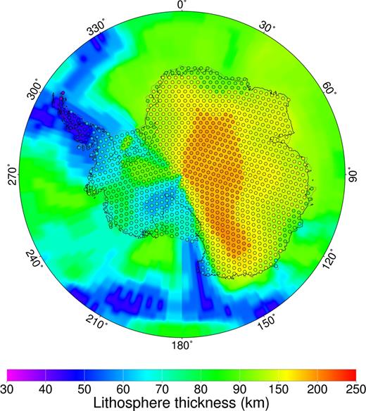
Thickness of elastic lithosphere (km) for the Antarctic region, as derived from Priestley & McKenzie (2013), and the thickness assigned in the inversion associated with the viscoelastic response function (circles).

4 RESULTS

4.1 Spatial rate of radial displacement

The total rate of radial displacement, |${\hat{y}^u}$|⁠, obtained in the joint inversion is shown in Fig. 8, as well as its separation into the elastic and viscoelastic components of the deformation. Note that ice shelves are assumed to be in floatation equilibrium; hence, the gravity signal recovered is attributed entirely to GIA, except where continental signals leak into the ice-shelf areas. A reference to the geographic locations of Antarctica discussed in the following can be found in Fig. 11. The strongest elastic response is localized in the Amundsen Sea Sector of West Antarctica, where large present-day mass losses cause strong rates of instantaneous rebound of the solid Earth. Localized rates of elastic uplift are also visible close to the tributary glaciers of the former Larsen B ice shelf on the Antarctic Peninsula. In contrast, bedrock subsidence is recovered in the area of the Kamb Ice Stream, caused by an increased ice build-up following the stagnation of this glacier system (Retzlaff & Bentley 1993). Large elastic rates are also visible around the GPS sites THUR, in the Bellingshausen Sea area, and SDLY, in Marie Byrd Land (see Fig. 10 for the locations of GPS sites).

Figure 8.

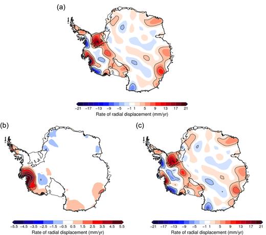
Rate of radial displacement (mm yr⁻¹) for (a) present-day ice-mass change and GIA (total), (b) present-day ice-mass change (elastic) and (c) the REGINA estimate of GIA (viscoelastic). Note different colour scale in (b).

The GIA-induced rates of radial displacement (Fig. 8) have two local maxima, one over the Filcher–Ronne ice shelf and one in the western part of the Amundsen Sea Embayment with rates above 10 mm yr⁻¹, which are discussed further in Section 4.3. The large uplift rates measured along the Transantarctic Mountains in central West Antarctica GPS (ca. 8 mm yr⁻¹) are mainly attributed to GIA, and they fill in along a stretch of uplift extending from the Ross ice shelf further inland. However, part of this signal is also attributed to elastic uplift caused by present-day snow/ice-mass changes, as seen in the altimetry data (see fig. 2 in REGINA paper I, Sasgen et al.2017). It should also be noted that, recently, problems of snow affecting the GPS receiver accuracy have been identified (Wilson, personal communication, 2016).

Another complication in the interpretation of GPS uplift rates arises from possible presence of co- and post-seismic bedrock deformation related to large earthquakes. King & Santamaría-Gómez (2016) have pointed out that the deformation signatures at Dumont d'Urville (DUM1), East Antarctica, contain abrupt offsets and relaxation behaviour related to the 1998 M ∼ 8.2 Antarctica intraplate Earthquake, with the epicentre about 600 km from the station (Nettles et al.1999). Furthermore, horizontal deformation associated with the 1998 earthquake has also been identified in the GPS record at Casey (CAS1), about 2000 km from the epicentre, suggesting that the deformation feature could be widespread, not only local (DeMets et al.2017). At DUM1, subsidence rates changed significantly from ca. 0.0 ± 0.5 mm yr⁻¹ (1993–1998) before the earthquake, to about −2.0 ± 1.0 mm yr⁻¹ (1998–2005) immediately after the earthquake, to about −0.2 ± 0.7 mm yr⁻¹ (2005–2015), after most of the post-seismic relaxation took place (taken from fig. 2 in King & Santamaría-Gómez 2016). Here, we adopt the rate of −0.3 ± 0.3 mm yr⁻¹ for the full GPS record at DUM1 (1995–2013), which is similar to the value during the Envisat/ICESat period (2003–2009) of −0.2 ± 0.7 mm yr⁻¹. It is also in agreement with the value of 0.0 ± 0.5 mm yr⁻¹ (1993–1998; before the earthquake), put forward by King & Santamaría-Gómez (2016) to be the most reliable.

East Antarctica shows uplift rates close to zero, however with some fluctuations of positive and negative rates. Contiguous, large-scale subsidence predicted by many models due to the increase of accumulation in the Holocene caused by the warming atmosphere and the associated increase in the water content and moisture transport. Subsidence in central East Antarctica is recovered in our solution, even though the stripy pattern may reflect noise. This is reflected in the rather large uncertainties for the East Antarctica presented in Section 5. The largest uplift rates are found in Wilkes Land, while Oates Land shows subsidence (geographic references are marked in Fig. 11). Most GIA corrections present a short-wavelength signal of uplift over the Totten glacier system, as a consequence of negative load change in the last 16 kyr in that region (e.g. Huybrechts 2002), supporting our GIA estimate in Wilkes Land. Note, however, that almost no ice history constraints exist for Wilkes Land to inform GIA modeling (Bentley et al.2014). The signature in Oates Land, however, is likely a result of an insufficient correction for surface-mass processes due to the lack of nearby GPS stations, as well as noise in the altimetry data caused by the rugged terrain (see fig. 2 from Sasgen et al.2017). A similar situation is present west of Amundsen Sea Embayment (Getz ice shelf area) and in eastern Bellingshausen Sea area, where the recovered GIA signal shows large rates of subsidence (ca. 15 mm yr⁻¹). It is likely that estimates of surface-mass loss from altimetry are too low in magnitude in the Getz ice shelf area due to the complex topography, as well as the difficult discrimination between ice shelf and grounded ice, and changes thereof. As these areas are underlain by a weak Earth structure, an insufficient correction for present-day ice-mass changes leads to large and spurious uplift rates. Along the Antarctic Peninsula, the terrain has a similar complexity; there, however, GPS uplift rates are more abundant and allow empirically improving the GIA estimate.

4.2 Spatial rate of geoid-height change

The rate of geoid-height change, |${\hat{y}^g}$|⁠, for the total mass change (recent and GIA-induced), as well as separated into present-day ice-mass change and GIA is shown in Fig. 9 . It should be stressed that the GIA-induced geoid rate is not derived by applying a conversion factor to the radial displacement field; it is derived in parallel to the radial displacement field based on the distribution of the viscoelastic response functions. For example, a locally high viscoelastic uplift rate may correspond to only a moderate increase in the geoid height, if the Earth structure attributed to this area is characterized by a thin lithosphere.

Figure 9.

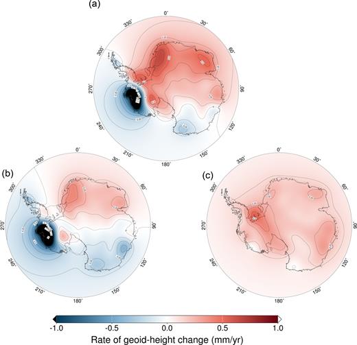
Rate of geoid-height change (mm yr⁻¹) for (a) present-day ice-mass change and GIA, (b) present-day ice-mass change and (c) the REGINA estimate of GIA.

The rate of geoid height attributed to present-day surface-mass change is dominated by the mass loss currently occurring in the Amundsen Sea Embayment. Here, geoid rates are by far the largest, amounting to several mm yr⁻¹. Marked ice losses are recovered along the northern part of the Antarctic Peninsula, as well as in Wilkes Land (Totten glacier) and George V Land, whereas mass increases due to the ice-dynamic slowdown of Kamb Ice Stream. Other signals of mass increase are recovered in Dronning Maud Land and Enderby Land, which is explained by enhanced accumulation within the considered time period. All these mass anomalies are known and have been related to their causative processes (e.g. Wouters et al.2014).

In contrast, the GIA-induced geoid rate is positive or close to zero over the entire continent of Antarctica, with the strongest magnitudes prevailing over West Antarctica. In East Antarctica, the radial displacement fields (Fig. 8) show some alternation between uplift and (smaller) subsidence, whereas the associated geoid pattern is generally positive, which is due to the overlapping with of positive geoid signals arising from the coastal rim in East Antarctica. Geoid rates peak at ca. 0.5 mm yr⁻¹ on the Filchner−Ronne ice-shelf area, but are also large for the Amundsen Sea and Ross ice shelf area, as well as in coastal East Antarctica along the western part of Wilkes Land and Enderby Land. In comparison to the present-day ice-mass changes, the recovered GIA signature has a distinct spatial pattern (peak anomalies in different locations) and it is smoother; this suggests that both signals have been successfully separated with no marked signs of correlation artefacts. In addition, the present-day ice-mass changes correspond in magnitude and spatial location to those inferred from the mass budget method (Rignot et al.2008, 2011b). The GIA-induced bedrock subsidence found in the hinterland of the Getz ice shelf (Fig. 8) is much less pronounced in geoid rate due to the thin lithosphere adopted in the viscoelastic response function for this area.

4.3 Large uplift in the Amundsen Sea Embayment

Next, we pay particular attention to the interpretation of the large uplift rates at the cm yr⁻¹ level measured by GPS in the Amundsen Sea Embayment; these cannot be explained solely by the elastic response to ongoing ice-mass unloading (Groh et al.2012). Seismic imaging (Hansen et al.2014), as well as inferences from radar sounding and subglacial water routing (Schroeder et al.2014) point towards a very low viscosity in the upper mantle of this region. Therefore, the large uplift is likely caused by a rapid viscoelastic response to more recent ice retreat and thinning. Due to the lack of geomorphological and climatological constraints on the ice evolution in the past few centuries to millennia, GIA forward models typically do not reproduce this uplift signature. With the joint inversion, we are able to reconcile with the large uplift, when considering the weak Earth structure in the determination of the viscoelastic response functions for this region.

A zoom into the displacement fields of Amundsen Sea Embayment at the respective disc locations of the geodesic grid (Fig. 8) are presented in Fig. 10. Overall, the total uplift obtained from the inversion is in very good agreement with the large uplift rates measured at the GPS stations, which is an indication that the applied smoothing constraint and viscoelastic response functions used in the inversion are adequate. Note that the GPS uplift rates determined here support earlier estimates based on campaign data at BEAR, PIG2 and MANT (Groh et al.2012).

Figure 10.

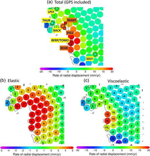
Rate of radial displacement (mm yr⁻¹) in the Amundsen Sea Embayment for (a) total signal (including GPS uplift rates as inset circles) comprising present-day ice-mass change and GIA, (b) present-day ice-mass change only and (c) GIA only. GPS sites used in the inversion (yellow label) are moved in location to the nearest node of the geodesic grid. Uplift rates provided by Groh et al. (2012) based on campaign data are shown for comparison at their true locations (brown labels). Note the different colour scale in (b). Numbers in the discs of (b) and (c) indicate the respective rates of radial displacement in millimetres per year.

Elastic uplift rates of 5–8 mm yr⁻¹ are determined for most of the Amundsen Sea Sector, as a consequence of ongoing glacier retreat and thinning. The uplift increases by ca. 2 mm yr⁻¹, when extending the time-series from the years 2003–2009 to 2003–2013 (not shown)—this is expected due to the acceleration of ice loss in this area. The GIA-induced signature shows uplift above 6 mm yr⁻¹ along the coast of the Amundsen Sea Embayment; peak rates of 18–19 mm yr⁻¹ are determined in the vicinity of the Thwaites and Smith/Pope/Kohler glaciers. The impact on the rate of geoid-height change is small, however, due to the thin elastic lithosphere in this region. As pointed out in the description of the viscoelastic response functions shown in REGINA paper I (Sasgen et al.2017), a moderate unloading in the past may cause substantial viscoelastic uplift if resting on a thin elastic lithosphere. Moreover, for upper-mantle viscosities of ca. 10¹⁹ Pa s (An et al.2015; Heezel et al.2016), the relaxation is fast enough that a new equilibrium state is achieved within a few centuries. Both properties of the Earth structure prevail in West Antarctica, suggesting that the isolated GIA signals are plausible.

It should be mentioned that the total uncertainty of GIA estimate in West Antarctica is large, due to the uncertainty in the altimetry data sets and the elevation rate to mass conversion (see Fig. 14). We have high confidence in our GIA estimate where GPS, altimetry and GRACE are co-located; but the regional spatial pattern, also in coastal West Antarctic, remains to be of a large uncertainty.

5 IMPACT ANALYSIS

5.1 Impact on altimetry and gravimetry trends

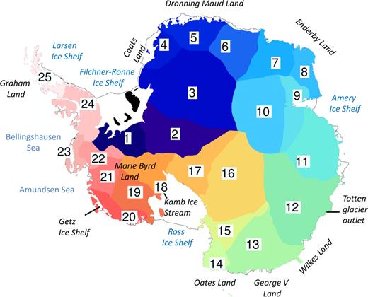
Next, we evaluate the impact of the GIA estimate on volume and mass balance estimates from satellite altimetry (Envisat/ICESat and CryoSat-2) and gravimetry (GRACE) estimates for the 25 Antarctic drainage sectors shown in Fig. 11. The results are shown in Table 1. In the following, basins 2–17 are considered to be part of East Antarctica, 1 and 18–23 are West Antarctica and basins 24 and 25 form the Antarctic Peninsula. The calculation of the of the volume rate |${\dot{V}_j}$| for a basin is straightforward; |${\dot{V}_j} = \mathop \sum \limits_i \hat{y}_{i,{\rm{GIA}}}^u{A_i}{\alpha _i}$|⁠, where i is the index of gridpoints within drainage basin j and A_i = const. = 100 km² is the nominal area represented by each gridpoint (here, 10 km × 10 km Polar Stereographic grid), while α_i accounts for the distortion of the true area with respect to the nominal area (α_i =  1 at true latitude of 71°S; range of ca. 0.87–1.06 within data domain). The gridded rate of radial displacement |$\hat{y}_{{\rm{GIA}}}^g$| is based on the GIA estimate shown in Fig. 8, however, interpolated bilinearly from the geodesic grid to the finer Polar Stereographic grid. The apparent mass change is determined by inverting the rate of geoid-height change, |$\hat{y}_{{\rm{GIA}}}^g$| (Fig. 9) to surface-mass change using a forward-modeling approach (e.g. Sasgen et al.2013).

Figure 11.

Outline of Antarctic drainage basins used in REGINA (after Sasgen et al.2013).

Table 1.

Apparent mean rate of volume (⁠|$\dot{V}$|⁠) change Envisat/ICESat (E/I; 2003–2009), extended with CryoSat-2 (CS-2; 2010–2013), and rate of mass (⁠|$\dot{m}$|⁠) change for GRACE (2003 January–2016 March; 152 monthly fields; CSR RL05), respectively, and the REGINA estimate for GIA-induced volume and mass change for each numbered basin in Antarctica (bold font) and uncertainties (light font).

Basin	E/I and CS-2	REGINA GIA		GRACE	REGINA GIA		Ice volume	Ice mass
number	(2003–2013)	volume estimate		(2003–2016)	mass estimate		(2003–2013)	(2003–2016)
	|${\dot{V}_{{\rm{altim}}}}.$|	|${\dot{V}_{{\rm{GIA}}}}$|⁠.	|$\sigma ( {{{\dot{V}}_{{\rm{GIA}}}}} )$|⁠.	|${\dot{m}_{{\rm{GRACE}}}}$|	|${\dot{m}_{{\rm{GIA}}}}$|⁠.	|$\sigma ( {{{\dot{m}}_{{\rm{GIA}}}}} )$|	|${\dot{V}_{{\rm{ice}}}}$|	|${\dot{m}_{{\rm{ice}}}}$|	|$\sigma ( {{{\dot{m}}_{{\rm{ice}}}}} )$|
2	−3	0.2	1.3	−2	4	4	−3	−6	5
3	24	0.2	1.5	16	5	7	24	11	7
4	13	0.6	0.7	10	2	3	12	7	3
5	14	0.3	1.2	12	2	4	14	11	5
6	20	0.5	1.1	9	2	3	20	7	3
7	6	1.2	0.9	15	4	3	5	12	3
8	7	0.6	0.7	13	2	2	6	11	3
9	3	−0.4	1.2	2	0	4	3	1	4
10	1	−0.1	0.9	3	0	4	1	3	4
11	−15	1.7	1.1	6	8	3	−17	−2	4
12	−43	2.6	1.7	−24	8	6	−46	−32	7
13	−11	0.1	1.1	0	1	3	−11	−1	5
14	12	−0.5	0.9	−7	−1	2	13	−5	3
15	−5	−0.2	0.8	1	0	3	−5	0	3
16	−3	−0.2	1.1	1	2	4	−3	−1	4
17	24	0.3	1	2	2	2	24	−1	2
East Ant.	25	7	4.4	58	42	15	18	16	17
1	−1	1.2	1.3	28	5	3	−2	23	4
18	26	1.1	1.4	15	5	3	25	10	3
19	−2	0.2	1.7	14	2	6	−2	12	8
20	−28	−0.6	1.3	−44	−3	5	−27	−41	7
21	−73	0.4	1.6	−62	2	7	−73	−65	7
22	−48	0	1.5	−53	0	7	−48	−53	8
23	−4	0.1	1	−12	0	5	−4	−13	7
West Ant.	−130	2.3	3.8	−115	12	14	−132	−127	17
24	−7	− 0.1	2.2	−8	1	9	−7	−9	10
25	−31	0.1	1	−20	1	4	−31	−21	4
Ant. Pen.	−39	0	2.4	−28	2	10	−39	−30	11
Total	−144	9.4	6.4	−86	55	23	−153	−141	27

Notes: Rate of ice-volume and ice-mass change are obtained by subtracting the GIA estimate from REGINA from the uncorrected satellite observations |${\dot{V}_{{\rm{altim}}}}$| and |${\dot{m}_{{\rm{GRACE}}.}}$| The GRACE uncertainties (1σ) are based on error propagation considering an AR(1) model (see the text), as well as filtering and inversion errors (typically 7–10 per cent; Sasgen et al.2013) and solution differences.

Typically, rates of ice surface-elevation change from altimetry are on the order of centimetres per year up to metres per year. In contrast, the GIA-induced bedrock uplift rates in Antarctica amount to a few millimetres per year, with a maximum of 2 cm yr⁻¹ in the presence of a thin lithosphere and low viscosity in West Antarctica. Therefore, GIA is not a primary correction or uncertainty for the satellite altimetry data. Integrated over the entire ice sheet the GIA impact is below 7 per cent of the volume rates (time interval 2003–2013), for the regions with large ice loss in West Antarctica even below 2 per cent. For East Antarctica, however, the relative contribution of GIA compared to the volume rates is significant, amounting to 30 per cent (Table 1).

Importantly, the GIA-induced mass change over Antarctica is similar in magnitude to the ice-mass change recovered by GRACE for 2003–2016: here we find it to be ca. 40 per cent of the latter. Overall, the mass-loss rates are roughly a minimum of four times more influenced by GIA than volume rates (the ratio of ice to rock density; Table 1). The uncertainty associated with our GIA estimate is ±23 Gt yr⁻¹ (⁠|${\sigma _{{{m'}_{{\rm{GIA}}}}}}$| for ‘Total’ in Table 1), which is about 16 per cent of the total GRACE uncertainty budget. However, it should be kept in mind that the range of published GIA corrections is considerably larger than this uncertainty, with values for the associated correction of mass change ranging from ca. +50 to +200 Gt yr⁻¹ (Martín-Español et al.2016b).

Note that the analysis of GRACE time-series for the extended time period 2003–2016 involves the simultaneous estimation of offset, trend, acceleration, as well as annual and semi-annual periods and the 161 d period (tidal aliasing in GRACE due to S2 tide; Chen et al. 2009). Following Williams et al. (2014), we select an autoregressive model of order 1, AR(1), as a single stochastic model, disregarding that other models may be optimal in different regions. Nonetheless, we estimate the statistical significance of the residual lag-1 autocorrelation, and if significant, scale the uncertainties using a pre-whitening procedure (Hamed & Rao 1998). The procedure increases the uncertainties of the trend typically by a factor of around 2, except for basins 1, 9, 10, 14 and 15, where we find residual correlation not to be significant.

5.2 Comparison with published GIA corrections

Next, we compare the spatial pattern of geoid-height change obtained in this study with the published GIA forward models (Fig. 12), W12a (Whitehouse et al. 2012) and the GIA inversion estimate based on pre-defined regional GIA patterns, AGE1 (Sasgen et al.2013). Further comparison is done for the rate of volume change for the 25 major drainage sectors (Table 1) shown in Fig. 11, including the GIA prediction IJ05_R2 (Ivins & James 2005; Ivins et al.2013), as well as the GIA estimates of Riva et al. (2009) and the RATES project (Martín-Español et al.2016a). Note that we compare our results to Riva et al. (2009) instead of the updated estimate presented in Gunter et al. (2014), as the latter involves an a priori constraint on the surface-mass balance in central East Antarctica. Thus, the comparison includes two GIA corrections based on modeling (W12a and IJ05_R2), which were favoured in the ice-sheet mass balance intercomparison exercise, IMBIE (Shepherd et al. 2012), and two inverse estimates (AGE1 and Riva et al. 2009). Although these models reflect much of the variability between GIA corrections at the scale of drainage sectors (Fig. 13 ), this comparison is by no means exhaustive. A more extensive comparison is provided elsewhere (Martín-Español et al.2016b).

Figure 12.

Spatial rate of geoid-height change (mm yr⁻¹) for (a) the GIA estimate of REGINA, (b) the GIA estimate AGE1 (Sasgen et al.2013) and (c) the GIA prediction W12a (Whitehouse et al.2012).

Figure 13.

Rate of volume change (km³ yr⁻¹) for 25 Antarctic drainage sectors (Fig. 11), as obtained from (a) REGINA, (b) AGE1, (c) W12a, (d) IJ05_R2, (e) Riva et al. (2009) and (f) RATES. For comparison, the REGINA estimate is also indicated as black bars in (b)–(f).

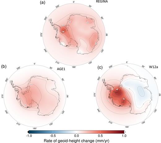
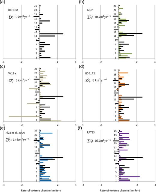
The GIA-induced rate of geoid-height change as obtained by the joint inversion, and for comparison the GIA prediction W12a and the GIA estimate AGE1 is presented in Fig. 12. Note that this version of AGE1 (‘GPS only’, table 2 of Sasgen et al.2013) is obtained by the adjustment of pre-defined GIA patterns to GPS uplift rates—no altimetry or gravimetry data were involved. All the GIA corrections show the largest uplift along a line joining the Filchner–Ronne and Ross ice shelves, West Antarctica. Also, the magnitudes of the inferred GIA are comparable and the GIA estimate of this study lies within the range provided by AGE1 and W12a. However, there are also marked differences: first, AGE1 and REGINA show a positive rate of geoid-height change over central East Antarctica, while W12 shows a decrease caused by viscoelastic subsidence due to enhanced accumulation, as a consequence of climate warming after the Last Glacial Maximum (e.g. Frieler et al.2015). Therefore, a subsidence signal is most likely realistic, and also present in the GIA prediction IJ02_R2 (not shown)—even though lower in magnitude than in W12a. The accuracy of our GIA estimate depends on the availability of GPS data, which are only located along the coastal rim in East Antarctica and the uncertainty of the elevation rates in the ice-sheet interior, which may be underestimated. Therefore, a subsidence signal in central Antarctica at the millimetre level is difficult to recover with the data-driven approach presented here. Fig. 13 compares the rate of apparent ice volume change for the 25 drainage sectors for AGE1, W12a and IJ05_R2 (Riva et al.2009), the inverse estimate of Martín-Español et al. (2016a), and the REGINA estimate of this study.

Typically, the volume rate is below 2 km³ yr⁻¹ and positive in magnitude for most drainage sectors. The exception is W12a, showing a strong negative GIA-induced volume change in Coates Land (basin 3), the Amery ice shelf area (basin 9) and part of central East Antarctica (basin 16). As mentioned in Section 4.1, our REGINA estimate also shows subsidence signals in the Getz ice shelf area (basin 20) and Oates Land (basin 14) and, in agreement with W12a, in the Amery ice shelf area (basin 9). In general, our REGINA estimate agrees best with Riva et al. (2009) and RATES, which is not surprising, as their GIA correction is based on a similar inversion approach using roughly the same type of input data sets. The GIA prediction IJ05_R2 is similar in large parts of Antarctica; however, a marked difference to the REGINA estimate (and that of Riva et al.2009) is the lack of uplift along Wilkes Land (basins 11 and 12), East Antarctica. This is also not supported by the GIA prediction W12a and may therefore be an artefact in our GIA estimate (and that of Riva et al.2009), caused by enhanced snow accumulation in the time period, which is captured differently by GRACE and Envisat/ICESat. Although all GIA corrections provide similar rates of volume change when integrated over the entire Antarctica continent, differences at the regional level remain large. The standard deviation between the GIA corrections is 0.3 km³ yr⁻¹ on average for all drainage sectors, but sometimes it is a large as 1–2 km³ yr⁻¹. Clearly, more research is needed to reconcile GIA estimates and GIA forward models on a regional level.

5.3 Uncertainties and limitations of approach to estimate GIA

The combination approach involves three different types of space-geodetic data: elevation rates from altimetry, gravity-field rates from GRACE and uplift rates from GPS station records. Using a bootstrap approach with 1000 samples of the likelihood distribution (mean and uncertainty) of the input data sets, we estimate the uncertainty of the GIA estimate (provided in Table 1), as well as the individual contributions shown Fig. 14. We perform the statistical sampling for individual data inputs, as well as for all inputs at the same time to account for possibly trade-off between errors from different sources.

Figure 14.

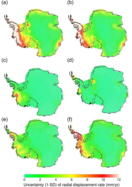
Uncertainty of the radial displacement of the GIA estimate and its individual contributions (mm yr⁻¹); (a) total uncertainty, and contribution from (b) altimetry (Envisat/ICESat; 2003–2009), (c) surface-density distribution, (d) GPS, (e) GRACE (magnitude of difference CSR RL05 and GFZ RL05) and (f) altimetry (Envisat/ICESat and CryoSat-2; 2003–2013; not used)

Among these three data sets, elevation rates from altimetry clearly pose the largest contribution to the uncertainties of the inferred GIA estimate. One reason is the sampling problem, which was partially alleviated by combining ICESat (high accuracy in coastal regions) and Envisat (smaller bias in central Antarctica). Our results show that further improvement is expected with CryoSat-2, particularly with its SARIn mode in coastal areas and possible swath processing, which provides denser elevation rate coverage around the ice margins where the largest rates are occurring (Gray et al.2013). Here, however, we refrain from including the CryoSat-2 data in the inversion, because the time span of the data set was insufficient to retrieve annual rates of surface-elevation change comparable to the other data set. In future, however, an updated GIA estimate will likely be possible by appending the time spans of different altimetry measurements.

Another major source of uncertainty is the conversion of ice surface-elevation rates to mass rates (Fig. 14). In our approach, outlined in Section 2, elevation changes are first corrected for firn compaction and then attributed to changes in snow and ice based on a pre-defined mask; after that, remaining surface-mass signals are identified by the joint inversion of GRACE and GPS data, and removed. However, this approach is limited by the spatial coverage of the GPS data.

Bedrock uplift rates derived from long-term and high-quality GPS records remain sparse in Antarctica (Fig. 4). Clearly, greater spatial coverage and longer time-series GPS data will improve the determination of GIA, as well as a better understanding of the spatial and temporal patterns of snow fall and ice-dynamic changes. Particularly, as many series of GPS sites provide only campaign measurements, further analysis is necessary of how interannual accumulation variations influence the derived rates and thus the GIA estimate. Nevertheless, Fig. 14 shows that except at a few sites, uplift rates from GPS are of sufficient accuracy to be valuable in a joint inversion GIA estimate, or for constraining GIA models.

The accuracy of the GRACE gravity fields is not a major limitation in the combination. In addition, it provides good spatial and temporal coverage. However, the coarse spatial resolution and principal problem of leakage currently limits our ability to derive small-scale signatures of GIA (and ice-mass change) with confidence. Note that in the Antarctic Peninsula, where the GRACE resolution is well below the length scale of GIA (ca. 100 km, good GPS coverage is helping to constrain our GIA solution (Nield et al.2012, 2014).

Finally, we have adopted viscoelastic response functions based on the equilibrium state for a constant unloading, removing all non-stationary characteristics of the temporal evolution. Even though the viscosity of the mantle underlying West Antarctica is probably low, this assumption may not be valid everywhere, which may lead to an overestimation of the recovered uplift rates. In addition, the Earth structure model adopted here (Priestley & McKenzie 2013) is subject to uncertainty. Nevertheless, we find that the choice of the Earth model parameters minimizes the misfit in both the GPS and gravity field rates and is therefore justified.

6 CONCLUSIONS

We have estimated GIA in Antarctica by the joint inversion of satellite altimetry, satellite gravimetry and GPS data. The inversion approach makes use of elastic and viscoelastic response functions to disc-load forcing, allowing us to partially account for lateral heterogeneous Earth structure in Antarctica and, in particular, a thin elastic lithosphere in West Antarctica. Including GPS uplift rates enables us to improve the separation of GIA and present-day ice-mass estimate, which initially rely on the surface-elevation rates from altimetry and an a priori snow/ice density distribution. Nevertheless, without further constraints on the spatial pattern of GIA, the uncertainty introduced by the altimetry data leads to a large uncertainty of the GIA estimate, also in West Antarctica (Fig. 14).

With the joint inversion, we successfully separate present-day ice-mass change and GIA, recovering a GIA estimate that is comparable in magnitude and spatial pattern to published GIA forward models, for example to IJ05 (Ivins et al.2013) and W12a (Whitehouse et al.2012) adopted in IMBIE (Shepherd et al. 2012). In total, the GIA-induced apparent mass change estimated is 55 ±  22 Gt yr⁻¹, which is identical to that obtained by an independent inversion approach using an entirely different methodology (RATES; Martín-Español et al.2016a), and in support of IJ05 and W12a. However, regionally, and at the basin scale, large differences in rate and apparent mass change exist between the REGINA and other recent GIA corrections for Antarctica. This suggests that, although both GIA inversion estimates and forward models can provide consistent results at the continental scale, large discrepancies remain at the basin scale, and the attribution to East and West Antarctica.

Isolated large uplift rates measured by GPS in the Amundsen Sea Sector are reproduced by the joint inversion using viscoelastic response functions, which account for a weak Earth structure in West Antarctica. We estimate that about two-thirds of the measured uplift in the vicinity of the Thwaites and Smith/Pope/Kohler ice streams is caused by GIA. We suggest that this uplift is due to ice retreat within the past few centuries rather than unloading at the millennial timescale following the Last Glacial Maximum. Further GIA modeling studies are necessary to reconstruct the temporal evolution of the ice sheet leading to a viscoelastic response that satisfies our satellite-based GIA constraint for Antarctica.

Applying the REGINA GIA correction to trends from GRACE monthly solutions for 2003 January to 2016 March yields a ice-mass loss of the entire AIS of −141 ± 27 Gt yr⁻¹. The regional separation exhibits a slightly positive mass balance of 16 ± 17 Gt yr⁻¹ for East Antarctica, a sustained negative balance of −30 ± 11 Gt yr⁻¹ for the Antarctica Peninsula and increasingly negative mass balances currently at a rate of −127 ± 17 Gt yr⁻¹ for West Antarctica.

Acknowledgements

The www.regina-science.eu work was enabled through CryoSat+ Cryosphere study funding from the Support To Science Element (STSE) of the European Space Agency (ESA) Earth Observation Envelope Programme. IS acknowledges additional funding through the German Academic Exchange Services (DAAD) and DFG grant SA1734/4–1. JLB and AME acknowledge additional support from UK NERC grant NE/I027401/1, and PJC and EJP from NE/I027681/1. We thank Erik Ivins, Riccardo Riva and Pippa Whitehouse for providing their GIA corrections, Thomas Flament and Frederique Rémy for the Envisat data and Veit Helm for providing the AWI L2 CryoSat-2 retracked and corrected elevation measurements. This work contributes to the Helmholtz Climate Initiative REKLIM (Regional Climate Change), a joint research project of the Helmholtz Association of German Research Centres (HGF).

SUPPORTING INFORMATION

Supplementary data are available at GJI online.

Figure S1. Spatial distribution and histogram of disc radii for geodesic grid applied in this study.

Figure S2. Discs of geodesic grid attributed to continental ice (blue; 1022 discs) and ice-shelf areas (magenta; 153 discs) in Antarctica.

Figure S3. Effect of regularization parameter on smoothness of GIA estimate. Shown is the spatial rate of radial displacement (mm yr⁻¹) for the (a) regularization parameter λ_N = 10^1.5, optimal for CSR RL05, 2003–2009 (nominal solution shown in Fig. 8), (b) λ_{N −} = λ_N · 10^{− 1.5} (less constrained; equivalent to L-curve optimal estimate), (c) λ_{N +} = λ_N ·  10^{+ 3} (more constrained), as well as (d) the difference of (b) minus (a) and (e) the difference of (c) minus (a).

Figure S4. Effect of the thickness of the lithosphere on of GIA estimate. Shown is the spatial rate of radial displacement (mm yr⁻¹) for the threshold viscosity value of (a) η_LT = 10²² Pa s (nominal solution shown in Fig. 8), (b) η_LT = 10²¹ Pa s (ca. 10 km thinner lithosphere in West Antarctica), (c) η_LT = 10²³ Pa s (ca. 10 km thicker lithosphere in West Antarctica), as well as (d) the difference of (b) minus (a) and (e) the difference of (c) minus (a).

Figure S5. Predicted rate of geoid-height change and rate of radial displacement for the equilibrium state and different lithosphere thicknesses (30:30–90:90 km). The dashed lines represent the measurements from GRACE and GPS at BERP/TOMO, Amundsen Sea Embayment, West Antarctica. The adopted Earth structure at this location (according to Priestley & McKenzie 2013) is 80 km. The a posteriori validation of the lithosphere thickness purely from the data at this location is 80–90 km.

Figure S6. Rate of surface-ice elevation change from Envisat/ICESat (E/I; 2003–2009; same as Fig. 3), from CryoSat-2 (CS-2; 2010–2013), as well as the mean trend from both altimetry fields (E/I and CS-2; 2003–2013). Note that for grid nodes without CS-2 data, E/I for 2003–2009 are adopted.

Table S1. Misfit of the prediction and observation for difference processing centres, cut-off degrees and the time intervals 2003–2009 (short) and 2003–2013 (long). The estimates were derived based on the individually optimized regularization parameter.

Table S2. Total misfit of the prediction and observation for difference Earth structure parameters. Indicated is the threshold value applied to the 3-D viscosity profile of Priestley & McKenzie (2013) for the definition of the elastic lithosphere (higher threshold means thinner lithosphere thickness). The misfit for including a ductile layer in the crustal part of the lithosphere is also listed (not further used in this paper; see REGINA paper I, Sasgen et al.2017). Results shown for GRACE solutions of CSR RL05, 2003–2009, cut-off degree 50.

Please note: Oxford University Press is not responsible for the content or functionality of any supporting materials supplied by the authors. Any queries (other than missing material) should be directed to the corresponding author for the paper.