Time-series analysis of abundance indices of young fish

Abstract

Catch-at-age analysis provides estimates of stock size at ages when the fish have reached catchable size. Survey indices contain information about relative cohort size at younger ages. The present analysis is concerned with survey indices of juveniles up to the youngest age where stock estimates, based on time-series analysis of catch-at-age data, are available. A stock estimate at that age from catch-at-age data is also included. A common model of the relationship between stock size and survey indices is combined with the model describing the decline of a stock by natural mortality. Random variations in natural mortality are defined separately from sampling variations and irregular catchability in the survey. The stock size and magnitudes of the random variations are estimated by the Kalman filter, which also provides predictions of future recruitment to the catchable stock. Analysis of observations of Icelandic cod reveals a large deviation from proportionality in the relationship between the index and the stock estimates in the youngest ages, but haddock data are compatible with proportionality. Variations in natural mortality during the second to fourth year of cod and the second to third year of haddock are not a major factor in variations of stock size.

1 Introduction

Survey indices provide information about relative stock size at the time of the survey. By combining this information with estimates of stock size from catch-at-age analysis, indices of younger fish can be used to predict recruitment to the catchable stock. Various statistical methods have been employed for this purpose (Rosenberg et al., 1992; Shepherd, 1997).

Myers and Cadigan (1993a, b) investigated survey indices of young fish from many stocks. Their analysis was mainly concerned with natural mortality and not with prediction of recruitment, and data or estimates from catch-at-age analysis were not included.

The present methodology is intended for stocks where annual survey indices can be obtained for a few years from each cohort before substantial exploitation begins. Catchability in surveys varies with age and size of the fish, particularly for the youngest ages. Before young fish enter the commercial fishery, their numbers decline due to natural mortality. The indices are subject to measurement errors and irregular variations in catchability. When a survey index is used to predict stock size at an older, catchable age, irregular variations in natural mortality between these ages contribute to the prediction error. With the time-series methodology, it is possible, at least theoretically, to estimate the magnitude of these variations separately from the irregular component of the survey indices.

We analyse in some detail abundance indices from a trawl survey on Icelandic cod in ages from 1 to 4 years from 1985 to 2002. For comparison with the results of Myers and Cadigan (1993a, b), we also include results from the analysis of haddock in ages from 1 to 3 years. The survey is carried out annually in March and was described by Pálsson et al. (1989). The cod data from the Marine Research Institute in Reykjavik (MRI, 2002, Table 3.1.10) are presented in Table 1. Estimates of the stock at 4 years of age, obtained by time-series analysis of catch-at-age data from the same report, are also included in Table 1. When the survey data become available, the last available catch-at-age data are from the previous year. The analysis is carried out in accordance with this, with catch-at-age results from 1985 to 2001. The main spawning period of Icelandic cod is in April. Notice that all fish hatched in year t are assigned age 0 during that year and 1 at the beginning of year t+1. Recruitment estimates provide additional information about the stock size at the youngest age in the catch-at-age analysis used in the management rules for this stock (Baldursson et al., 1996). Predictions made further ahead affect economic planning by fisheries and the government.

Table 1

Survey indices of Icelandic cod for ages 1–4 and estimates of stock size at age 4 from catch-at-age analysis.

	Survey indices
	Age 1	Age 2	Age 3	Age 4	Stock (million fish)
1985	16.54	112.3	35.4	48.2	104
1986	15.10	61.0	95.7	22.5	108
1987	3.65	28.9	104.0	83.5	248
1988	3.45	7.5	72.7	104.9	206
1989	4.09	17.3	22.4	80.1	131
1990	5.57	12.1	26.7	14.3	68
1991	3.95	16.3	18.2	30.7	102
1992	0.72	17.5	33.8	19.1	75
1993	3.58	4.8	35.1	39.3	135
1994	13.76	16.0	8.9	27.1	98
1995	1.17	29.3	26.2	9.4	57
1996	3.63	5.4	41.9	28.3	126
1997	1.21	22.4	13.7	56.5	133
1998	7.98	5.5	29.8	16.0	73
1999	7.38	34.3	7.1	42.3	140
2000	18.81	28.5	55.6	7.2	46
2001	12.09	24.1	37.0	38.3	145
2002	0.91	38.7	41.2	40.3

The relative magnitudes of the survey indices for cod at each age vary much more than the stock estimates. Higher irregular variations of the indices may have some part in this, but visual examination of Table 1 shows that it is mainly a systematic feature of the data; an index of a cohort that is large or small in any particular year in the indices, retains its relative position during the 4 years included here.

2 Model

The number of fish is treated as a continuous variable and the basic model of change in cohort size is

where N is the number of fish and Z is the rate of mortality. For interpretation of annual data, it is customary to solve the equation, assuming that Z is constant during the year, so that

(1)

N_at is the number of fish of age a at the beginning of year t and Z_at is the mortality rate of fish of age a during year t.

In the present work, observations consist of survey indices of year-class strength of young fish. One series of estimates of the stock size in numbers in the youngest age where substantial commercial catches begin is also included. This series is based on catch-at-age analysis. They are highly variable in magnitude. In order to stabilize variances and bring them closer to normality, it is convenient to work with logarithmic values and we denote the logarithmic stock values by n_at. The indices are related with the stock values through the model

(2)

The logarithmic value of the index is i_at. Catchability of the survey (q_a) varies with age and we also allow for variation with stock size by the parameter ϕ_a. Irregular variations in catchability are indistinguishable from measurement errors and we include both in the residuals ɛ_at, defined as serially uncorrelated, normally distributed with zero mean and variance σ_ɛa².

The actual age range will usually be from 0 or 1 to an age A, where estimates of stock size can be obtained from catch-at-age analysis. We cannot estimate absolute stock size in the ages below A from these data without some further information about the magnitude of catchability or mortality. No such knowledge will be assumed here.

Let us first ignore the possibility that natural mortality depends upon stock size and separate systematic and random variations,

(3)

where ξ_a is a constant age-dependent mortality rate and ζ_at represents random variations in the mortality, assumed to be normally distributed, serially uncorrelated with zero mean. From Equations (1) and (3) we obtain

(4)

Suppose now that N_at is known in year t and denote the expected log-value of the cohort when it reaches age A by r_at,

(5)

From Equations (2) and (5) we obtain

(6)

Without some external knowledge about the magnitude of catchability and mortality at each age we cannot separate these effects with the present data so we simplify the measurement equations of the indices to

(7)

where the constants Q_a include effects of both age-dependent catchability and mortality.

At age A, the stock has been estimated from catch-at-age analysis. We regard these estimates as observations and denote them by a hat,

(8)

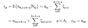
The errors, ɛ_n,t, are defined as normally distributed, independent of ɛ_at and serially uncorrelated.

The unobserved variables r_at are called state variables. Their true values are connected by the relationship

(9)

The residual δ_at=ζ_a−1,t−1, i.e. the difference between r_at and r_a−1,t−1, consists of the irregular component in the natural mortality at age a−1 during year t−1. A separate equation must be defined for the youngest age included in the analysis. Let this be a=1. From Equation (5) we have

(10)

The age-dependent mortality rates ξ_1+i are unknown constant values. The simplest assumption about the unknown values of n_1t is that they are independent, normally distributed with a fixed mean, n₀, and variance σ_δ1². However, in the present analysis it is not possible to estimate n₀ separately from the unknown value of ∑_i=0^A−2ξ_1+i and we define

(11)

and

(12)

where the residuals δ_1t have variance σ_δ1². This equation represents our knowledge about the respective cohort before the first observation from it in the survey data, i.e. i_1t. The model could be expanded to include information from a stock-spawning relationship or possible trend but this will not be considered here. The residuals δ_1t represent irregular variations in spawning and natural mortality before fish reach age 1.

Natural mortality could depend upon stock size as discussed by Myers and Cadigan (1993a). This can be expressed in various ways, but for the present estimation procedure a convenient model is

(13)

where r_at is now the expected cohort size at age A apart from the stock-dependent variations in natural mortality, represented by γ(r_a−1,t−1−r₀).

3 Estimation

The unobserved series of state variables, r_a,t, are estimated from the observed indices and the catch-at-age estimates at age A by means of the Kalman filter. As the present models are linear in the state variables, no modification or extension of the Kalman filter is needed. This algorithm proceeds from initial values by predicting the state variables r_at in the next period by their models with the expected value 0 inserted for the residuals δ_at. The predicted values of r_at are used to predict the observed indices and according to the models in Equations (7) and (8) and to calculate the prediction errors. These errors contain information about the estimates of state variables employed in the predictions. An overprediction of i_at in Equation (7) indicates that r_at was too large and should be adjusted. But the random element, represented by ɛ_at, also contributes to the prediction error of i_at. If the variance of ɛ_at is large, compared with the uncertainty of the state variable, the adjustment should be small. The function of the Kalman filter is to determine the appropriate updating of the state variables in accordance with the prediction errors of the measurements and to calculate the covariance matrix of the updated estimates. A formal description of the application of the Kalman filter to the present model is given in Appendix 1.

In order to apply the Kalman filter, we need initial values of the state variables in ages from 1 to A−1 years in the year before the first observations. All parameters in Equations (7), (8), (9), (12), and (13) must be known, including the full specification of the covariance matrices of δ_at and ɛ_at. In reality, these parameters are not known but can be estimated by the likelihood function of the prediction errors, i.e. we find the parameters by which the Kalman filter produces the best predictions of i_at and ⁠. Approximate standard deviations of estimated parameters are obtained from the Hessian matrix. The estimated covariance matrix of the state variables does not include uncertainty in parameter estimates and tends to underestimate the actual uncertainty, but not by an order of magnitude.

The direct estimation of the stock in Equation (8) is obtained by time-series analysis of the catch-at-age data (Gudmundsson, 1994). The best estimates of this stock at catchable ages are obtained from a joint analysis of these data and the survey indices. However, the uncertainty in specifying the correlation between ɛ_n,t from a joint analysis and the residuals ɛ_at in Equation (2) counteracts this advantage. In the present analysis, we use stock estimates obtained without using data other than the catch-at-age where we can safely assume that there is no correlation with ɛ_at. It is only in the last years that substantial differences may emerge between different estimation procedures.

Time-series estimation of n_At from catch-at-age data also provides estimates of the standard deviation of this estimate. But this estimation is rather inaccurate. It depends upon the method used for stabilizing variances and various somewhat arbitrary specifications of covariance matrices. Estimates of stocks and mortality rates in the last year are less accurate than in previous years, but the reverse applies to the assessment of the accuracy. In the present analysis, the standard deviation of ɛ_n,t in the last year, 2001, is obtained from the catch-at-age analysis. The standard deviation from 1985–1997 is estimated as a constant value σ_n, and the values from 1998–2000 as a linear interpolation between σ_n and the value in 2001.

The number of parameters is high. With four ages included there are two 4×4 covariance matrices, two parameters, Q_a and ϕ_a, for each age in the measurement equations for the indices, and σ_n, r₀ and γ. With T years of observations the size of T+A−1 cohorts must be determined, although only the A−1 initial values of r_at enter as separate estimated parameters. The number of quantities to be determined is thus very high compared with the number of observations, but this is a common feature of cohort analyses of fish stocks.

It is necessary to introduce various simplifications in order to keep down the number of parameters and obtain well-determined estimates. The likelihood function is used to test the validity of parameter restrictions. The next section describes the specification and estimation with observations of Icelandic cod. Much of this will be common with data from other stocks, but not necessarily every detail.

The values of r_aT, obtained by the Kalman filter in the last year of observation, are our predictions of the recruitment to the stock at age A in the years from T to T+A−1, based on the whole data set. The Kalman filter estimates of r_at in earlier years are based on the data up to and including year t. However, subsequent observations contain further information about these values. Estimates of r_at, based on the whole data set, are obtained by a recursive procedure called “smoothing”.

Examination of residuals is an important aspect of applied time-series analysis. Observed residuals are the difference between the observed series and values predicted by the models. In the present analysis, the residuals are the prediction errors of i_at and one year ahead. They are composed of the stochastic elements represented by ɛ_at and ɛ_nt in Equations (7) and (8) and also the errors produced by inaccurate estimation of the state variables r_at. The residuals should be serially uncorrelated with all other residuals, but correlations of the prediction errors at different ages within the year are allowed in the model.

The prediction errors should have zero mean, but the variances differ in accordance with the different variances of the residuals in Equations (7), (8), (9), (12), and (13). The calculated residuals are therefore standardized by dividing by the calculated standard deviation of the respective residuals. Test statistics are calculated jointly for the standardized residuals from Equation (7). Two test statistics for normality are calculated, g₁ for skewness and g₂ for kurtosis. Both are approximately distributed as N(0;1) under the null hypothesis of normal distribution of the residuals. Two first-order serial correlation coefficients, r_t and r_c, are calculated. They represent the correlation between the residual at (a,t) with the residuals at (a,t−1) and (a−1,t−1), respectively. They are approximately normally distributed with zero mean and variances {A(T−1)}⁻¹ and {(A−1)(T−1)}⁻¹ under the null hypothesis of no serial correlation (Gudmundsson, 1986).

The Kalman filter, parameter estimation, and smoothing are described in textbooks on time-series analysis (e.g. by Harvey, 1989).

4 Examples

We describe here in some detail the parameter estimation and recruitment prediction of Icelandic cod. Parameter estimates for Icelandic haddock, obtained by similar methods, are also presented.

The survey indices of Icelandic cod in Table 1 are calculated in the same way at all ages. Most of the spawning takes place in the weeks immediately after the survey so the youngest age sampled in this survey is 1 year. There is a 0-group survey in August (Astthorsson et al., 1994). The 0-group index is more volatile than the trawl survey indices, and possible misspecification of the relationship with the stock values, including the stochastic aspect, could be damaging for the analysis. It is therefore not included in the present analysis, although the results convey some information about cohort strength.

The standard deviation of the stock estimation at 4 years of age in 2001 from the catch-at-age analysis is 0.17 and the present estimation of σ_n from 1985–1997 is 0.105 (Table 2). This estimate is too high according to the catch-at-age analysis, but as other results are not much affected if we use a lower value for this parameter, only results obtained with this value of σ_n will be presented. As refers to the stock at the beginning of the year, the residuals ɛ_nt also include irregular mortality until the survey is carried out. But this is not a major factor because catches of 4-year-old cod are small during this period. The assumption of no serial correlation of the residuals in Equation (6) is incorrect for the last values, but they have bigger variances and thus exert less influence upon the results.

Table 2

Parameter estimates and residual statistics. θ is estimated and γ is fixed in the first cod-column and in the haddock-column. In the second cod-column, θ is fixed and γ is estimated. Estimated standard deviations of the parameters are presented in parentheses below the respective parameter values.

	Cod	Cod	Haddock
σɛ1	0.276	0.285	0.200
	(0.100)	(0.090)	(0.094)
σɛ,2−A	0.068	0.071	0.000
	(0.058)	(0.058)	(0.109)
σκɛ	0.159	0.158	0.214
	(0.037)	(0.038)	(0.098)
σδ1	0.387	0.515	0.735
	(0.100)	(0.106)	(0.267)
σδ,2−A	0.069	0.072	0.082
	(0.026)	(0.030)	(0.085)
σκδ	0	0	0
σn	0.106	0.105	0.160
	(0.023)	(0.026)	(0.051)
ϕ1	2.31	1.75	0.93
	(0.29)	(0.15)	(0.49)
θ	−0.189	0	0.066
	(0.089)		(0.071)
γ	0	−0.091	0
		(0.035)
g1	−0.61	−0.61	0.08
g2	−1.48	−1.49	−1.29
rt	0.04	0.04	−0.13
rc	−0.17	−0.15	0.10

σ_ɛa: measurement errors and variations in catchability at age a; σ_κɛ: joint variations in catchability; σ_δa: irregular variations in natural mortality at age a; σ_κδ: joint irregular variations in natural mortality; σ_n: errors in stock estimates from catch-at-age analysis at 4 years' age; ϕ₁: constant in a model of stock-dependent catchability; θ: coefficient of age in a model of stock-dependent catchability; γ: coefficient in age-dependent natural mortality; g₁: test for skewness, N(0;1); g₂: test for kurtosis, N(0;1); r_t: test for first-order serial correlation in time, N(0;0.12²) for cod, N(0;0.14²) for haddock; r_c: test for first-order serial correlation within cohorts, N(0;0.14²) for cod, N(0;0.18²) for haddock.

For Icelandic cod, we use A=4 years and must then specify and estimate the 4×4 covariance matrix of the residuals ɛ_at in Equation (2). These residuals represent measurement errors and variations in catchability. We know from analysis of catch-at-age data and survey indices that estimation of joint variations in catchability from ages 4 to 9 years yields large and highly significant values (Gudmundsson, 1998). The convenient prior assumption of independent residuals is therefore inappropriate.

Estimation of six covariances for the measurement equations with these data is not feasible; one parameter must suffice to account for possible correlations. The present specification defines all ɛ_at as independent and adds an extra residual, κ_ɛt with variance σ_κɛ², to Equation (7),

(14)

The total variance of the residuals at age a is then σ_ɛa²+σ_κɛ² and the covariances are all σ_κɛ². The covariance matrix of the residuals of the state variables is defined in the same way by adding κ_δt to Equations (9), (12), and (13).

The standard deviation of ɛ_1t, representing measurement errors and catchability variations in the survey for the 1-year-old fish, is much higher than for the older fish. The possibility that the large variations at 1 year of age are not highly correlated with variations in the older ages was investigated by excluding κ_at when a=1 and found to fit better. The results for cod presented in our tables were obtained with this option. The residual variations at older ages are highly correlated, indicating that variations in catchability are more important than sampling variations. The possibility of defining the covariance matrix with correlations declining with increasing age-difference was also investigated, but the present formulation was easier to estimate and fitted slightly better.

Free estimation of the ten parameters, σ_ɛa, σ_κɛ, σ_δa, and σ_κδ produces rather badly determined values for most parameters. But the restriction to use the same parameter for the standard deviation of ɛ_at for ages 2–4 years and another for δ_at in these ages is acceptable (log L drops by 2.9).

According to the estimated values (Table 2), the variations of natural mortality, represented by σ_δ,2–4, are much lower than variations in stock size at age 1, represented by σ_δ1. The variations in cohort size at 4 years of age are therefore dominated by variations in spawning and natural mortality in the first year. There is no indication of correlation within each year between the residuals δ_at, associated with variations in natural mortality, regardless of the choice of specification.

We are estimating recruitment to A=4 years for cod in this study but there are also some recorded catches in younger ages. The effect of correcting for catches at 3 years was investigated but had negligible effect upon the goodness-of-fit and did not improve it. The correction was not applied in the results presented here. Unrecorded discards are equivalent to natural mortality in this analysis. Although we cannot determine relative variations in catchability in the younger ages without knowing the natural mortality rate, it is obvious from Table 1 that catchability at 1 year of age is much lower than in the higher ages.

The parameters Q_a are estimated separately at each age, but as we do not know the relative contribution of regular variations with age in catchability and natural mortality, the values are of little interest. The estimated values of ϕ_a are of the order of 2 and the log-likelihood function drops by about 30 by fixing all ϕ_a=1. The plausible assumption of proportionality between index and stock size is therefore incompatible with these data. But a linear change of ϕ_a with age is acceptable so we can represent the four values by two parameters,

(15)

The estimated values of θ in Table 2 are obtained by assuming that natural mortality is not stock-dependent, i.e. with γ=0. Joint estimation of θ and γ results in insignificant values of both parameters. The negative value of θ implies that stock-dependent catchability decreases with increasing age. For cod, results of estimation with θ fixed at 0 are also presented in Table 2. A negative γ implies that natural mortality of large cohorts is higher than for small cohorts. Most other parameters are little affected by which of the variables θ or γ is included, but the initial stock-size variation, represented by σ_δ1, is bigger with γ. The variation subsequently decreases with age because of the stock-dependent mortality. Note that ϕ₁ is much bigger than 1 so that the catchability is still strongly stock-dependent. Log L differs by 0.2 depending on whether γ or θ is estimated, which is negligible. It is therefore not possible, with the present data and models, to distinguish between variation with age of stock-dependent catchability in the survey, and stock-dependent natural mortality.

The smoothed estimates of r_at, obtained with γ=0, are presented in Table 3, transformed from logarithmic values to stock size in numbers. The variations in these values within each cohort represent the estimated effects of the irregular variations in natural mortality, denoted by δ_at in Equation (9). The same estimates, obtained with stock-dependent natural mortality, are presented in Table 4. The variations within cohorts in this table are the estimated effects of stock-dependent and irregular variations in natural mortality.

Table 3

Smoothed estimates of exp(r_at) for Icelandic cod when variation with age of stock-dependent catchability is estimated.

	Million fish
Year	1-yr olds	2-yr olds	3-yr olds	4-yr olds
1985	201	225	101	117
1986	154	211	217	101
1987	77	152	221	217
1988	94	73	162	215
1989	92	94	77	156
1990	107	90	101	71
1991	104	106	84	106
1992	54	106	112	81
1993	101	55	107	117
1994	145	103	57	102
1995	64	142	105	57
1996	107	65	137	111
1997	59	111	67	139
1998	139	58	107	70
1999	131	143	50	121
2000	145	133	144	47
2001	158	137	132	139
2002	56	161	132	131

Table 4

Smoothed estimates of exp(r_at) for Icelandic cod when variation with age of stock-dependent natural mortality is estimated.

	Million fish
Year	1-yr olds	2-yr olds	3-yr olds	4-yr olds
1985	254	266	101	117
1986	176	245	234	101
1987	69	165	238	217
1988	91	68	170	215
1989	87	93	74	156
1990	109	87	100	71
1991	105	107	82	106
1992	44	106	113	81
1993	101	48	108	117
1994	161	103	53	102
1995	55	151	105	57
1996	109	59	142	111
1997	49	112	64	139
1998	156	52	108	70
1999	143	154	47	122
2000	160	140	149	47
2001	183	146	135	138
2002	46	177	136	131

The Kalman filter provides standard deviations of the estimated values of r_at. They refer to the relative size of the cohort at age a in year t. These values are also predictions of the size of the cohort when it reaches age A but the standard deviations of the predictions are bigger because of irregular variations in natural mortality from t until t+A−a. In the estimation with γ=0, these standard deviations for cod are as follows:

The last row of Table 3 shows the predictions of the stock size at 4 years of age in the years 2005, 2004, 2003, and 2002, obtained from the survey values of 2002. Table 5 shows similar predictions obtained with survey indices ending in 1998–2002 and the corresponding stock estimates ending in 1997–2001. The specifications were the same as in Table 3, but the parameters were reestimated for each data set.

Table 5

Recruitment predictions of Icelandic cod at age 4 years.

	Million fish
	exp(r1T)	exp(r2T)	exp(r3T)	exp(r4T)
1998	127	62	106	67	73
1999	126	143	55	111	140
2000	189	138	148	50	46
2001	151	143	135	141	145
2002	56	160	132	131
σ(pred)	0.18	0.11	0.09	0.06

The Kalman filter provides estimates of the standard deviation of r_aT but the error in the prediction of the logarithmic value of the stock at 4 years of age also includes the uncertainty caused by irregular natural mortality. This is included in σ(pred).

For comparison with these results and the results from Myers and Cadigan (1993a, b) we also analysed haddock indices from the same survey. The time period was the same but the age range was from 1 to 3 years. The estimated standard deviation of the log-value of the stock at 3 years of age in 2002 from catch-at-age analysis was 0.23. Catchability of haddock at 1 year of age is much higher than for cod and the joint variations in catchability, represented by κ_ɛt, were included at all ages. No evidence of stock-dependent catchability or natural mortality appears in the haddock results, i.e. ϕ₁ is not significantly different from 1 and θ and γ are not significantly different from 0.

The test statistics show no evidence of non-normality or serial correlation in the analyses of these data sets.

5 Discussion

The data employed in the present work could also be used with other methods currently applied to predict recruitment. But unless random variations of natural mortality and joint catchability variations are negligible, these methods are not fully efficient because assumptions of independent residuals in their specifications are violated.

Our description and examples of this procedure were in terms of indices from a single survey. The basic theory is the same with indices from more than one survey for some or all of the ages, provided they are carried out at the same time. In view of the large correlations between the residuals associated with the present survey indices, the possibility of correlations between indices of different surveys should be investigated and taken into account. There are no methodological difficulties in carrying this out.

Joint analysis of indices from surveys, carried out at different times in the year, requires more extensive modification of the methodology. In order to keep variations in natural mortality separate from measurement errors and variations in catchability, the state variables r_at should be updated at the time of each survey so we would no longer be working with time intervals of 1 year. However, the results of Myers and Cadigan (1993b) and the present paper indicate that irregular variations in natural mortality may often be so small that it is harmless to ignore them in recruitment predictions. It is not necessary that each survey includes all ages or that they all start in the same year.

Our results for cod differ in two respects from those of Myers and Cadigan (1993a, b). We find a small but significant irregular variation in natural mortality and a strong stock-dependence in catchability. In both cases, the difference rests upon the information in the series of stock estimates from the catch-at-age data, included in our analysis but not in the work of Myers and Cadigan. If we reduce the effect of this series by assigning a bigger variance (σ_n²) to the stock estimates, the estimated variance in natural mortality (σ_δ,2–4²) becomes insignificant. Myers and Cadigan (1993a) assume that the estimated abundance in the survey is proportional to the true abundance, i.e. ϕ₁=1. According to our results, this assumption is untenable for Icelandic cod. However, this conclusion also rests upon the information from the catch-at-age estimation. It was carried out with the traditional assumption of a constant natural mortality (0.2 year⁻¹) in the catchable ages. If this assumption is wrong and the natural mortality is in fact strongly stock-dependent, then the stock estimates, based on the assumption of a constant natural mortality, are systematically wrong and the evidence for stock-dependent catchability could vanish. It is difficult to estimate the magnitude or the variations in natural mortality in ages with high fishing mortality. At the moment, we have no presentable evidence for or against the hypothesis of stock-dependent natural mortality of Icelandic cod in the catchable sizes and ages (>50 cm, ≥4 years).

For Icelandic haddock, we find no significant irregular variation in natural mortality. The precision of this estimation is lower for haddock than for cod because we have one age less in the survey data and less accurate catch-at-age estimates. It is therefore not possible to infer from the present analysis that the actual variations are in fact smaller for haddock than for cod. There is no indication of stock-dependent catchability or natural mortality for haddock. This is in agreement with the results from most of the haddock stocks investigated by Myers and Cadigan (1993a). In view of the difference between the results from Icelandic cod and haddock in these respects, it is worth noting that catchability in our survey is much higher for haddock than for cod. The stock in numbers of cod is bigger than the stock of haddock, but the survey catches five times more haddocks than cods.

Appendix 1

The Kalman filter algorithm

For each year, we have a vector of observations,

The observed series are connected with the unobserved series of state variables,

by the relationship

The coefficient matrix H is determined by Equations (7) and (8). The diagonal elements are ϕ_a in the first A rows. The Ath element in row A+1 is 1. All remaining elements are 0. The first A elements of the vector Q are Q_a and the last is 0. The residuals have covariance matrix E_t. The first A rows and columns are occupied by the covariance matrix of the residuals ɛ_at. The last diagonal element is the variance of ɛ_n,t and the off-diagonal elements in the last row and column are 0 if the stock estimates are independent of the survey indices.

The state vectors in year t are connected with previous values by

The coefficient matrix G has elements g₂₁=…=g_A,A−1=1 and the remaining elements are 0. The first element of the vector r₀ is r₀ and the remaining elements 0. The covariance matrix of δ_t is D_t.

Suppose now that we have estimated r_t−1 by with covariance matrix P_t−1. We can then predict the next state variables by

The error of this estimate has covariance matrix

We predict the vector of observations in year t by

The prediction errors,

have covariance matrix

The prediction errors contain additional information about r_t and we update the predicted value by

with covariance matrix

The log-likelihood function is