Variability in the density and sound-speed of coastal zooplankton and nekton

Abstract

Forman, K. A., and Warren, J. D. 2010. Variability in the density and sound-speed of coastal zooplankton and nekton. – ICES Journal of Marine Science, 67: 10–18.

Acoustic sampling techniques provide an advantage over traditional net-sampling by increasing scientist ability to survey a large area in a relatively short period, as well as providing higher-resolution data in the vertical and horizontal dimensions. To convert acoustic data into measures of biological organisms, physics-based scattering models are often used. Such models use several parameters to predict the amount of sound scattered by a fluid-like or weakly scattering animal. Two important input parameters are the density (g) and sound-speed (h) contrasts of the animal and the surrounding seawater. The density and sound-speed contrasts were measured for coastal zooplankton and nekton species including shrimps (Palaemonetes pugio and Crangon septemspinosa), fish (Fundulus majalis and Fundulus heteroclitus), and polychaetes (Nereis succinea and Glycera americana) along with multiple physiological and environmental variables. Factors such as animal size, feeding status, fecundity, gender, and maturity caused variations in g. The variations in g observed for these animals could lead to large differences (or uncertainties) in abundance estimates based on acoustic scattering models and field-collected backscatter data. It may be important to use a range of values for g and h in the acoustic scattering models used to convert acoustic data into estimates of the abundance of marine organisms.

Introduction

Acoustic sampling techniques are an important tool for studying the marine environment, allowing scientists to assess large areas of the ocean rapidly to ascertain the abundance and, in some cases, the composition of the zooplankton community. A critical step in the process is the conversion of the amount of scattered acoustic energy from water-column targets to abundance or biomass estimates (Foote and Stanton, 2000). The use of acoustic backscatter as a measure of biological organisms is an indirect method that requires the identification of the scattering targets by a direct method such as a net tow or optical imaging system. However, a major benefit of acoustic techniques is that they allow scientists to survey a large area of the water column in a relatively short period with greater resolution in both horizontal and vertical dimensions (Traykovski et al., 1998; Chu et al., 2000a; Warren et al., 2003).

To convert acoustic backscatter into biological information, scattering models are used to predict how much acoustic energy a single animal of a particular body structure (e.g. fluid-like, gas-bearing, or elastic-shelled) will scatter (Stanton et al., 1998a; Foote and Stanton, 2000; Brierley et al., 2005). These theoretical scattering models are tested under both laboratory and field conditions and require knowledge of several input parameters in order for them to describe the scattering accurately. For the acoustic frequencies commonly used in echosounder surveys (tens to hundreds of kilohertz), an animal's target strength (TS), or its efficiency in backscattering sound, depends primarily on its body structure, shape, size, orientation, and material properties, as well as on the acoustic wavelength and frequency.

The material properties include the density contrast (g) and sound-speed contrast (h) of the scatterer relative to the surrounding medium (Stanton et al., 1998b), both of which are of importance in TS models (Stanton et al., 1996; Chu et al., 2000a; Demer, 2004; Lawson et al., 2006). Prior knowledge of these properties is necessary to make the conversion from TS to biological quantities. As animals are often more dense than seawater, g is typically >1 (Greenlaw, 1977); however, values of g used previously for fluid-like zooplankton range from 0.9862 to 1.0622 (Chu et al., 2000a). Sound travels faster through a denser medium, so h will typically be >1; however, values of h used previously range from 0.9978 to 1.0353 (Chu et al., 2000a).

Small changes in g and h can change TS significantly (Greenlaw, 1977; Greenlaw and Johnson, 1982; Chu et al., 2000b), leading to greater uncertainties in estimates of biomass and abundance (Greenlaw, 1977; Chu et al., 2000a). Therefore, it is important to understand how the material properties are affected by biological and environmental conditions and the physiology of the animal (Chu et al., 2000b). Current methods for calculating TS use scattering models that assume constant values of g and h for all animals of a particular species or size class. However, earlier studies (Chu et al., 2000b; Chu and Wiebe, 2005; Warren and Smith, 2007) show evidence that this may not be an accurate representation because the values of g and h vary from one animal to another.

The focus of this study was to measure values of g and h for several coastal zooplankton and nekton species and to determine how physiological or environmental factors may affect the values. The animals were selected for study because they are locally abundant and easily collected. Although they are not phylogenetically similar, they are similar in shape, size, and scattering characteristics to such ecologically important or abundant pelagic zooplankton species as euphausiids, fish larvae, and marine worms. In addition, this study examines the effect of using a single value of g and h vs. a more realistic distribution of values of g and h when using scattering-model results to convert measured acoustic backscatter values into biologically meaningful information.

Methods

Shrimps (Palaemonetes pugio and Crangon septemspinosa), fish (Fundulus majalis and Fundulus heteroclitus), and polychaetes (Nereis succinea and Glycera americana) were collected from autumn 2006 through summer 2007 from various bays on the coast of Long Island, NY, USA. The shrimps and fish were collected either with a seine-net from the shore at Flax Pond Marine Laboratory, Hampton Bays (HB), Shinnecock Bay (SB), and Patchogue or with a bait trap deployed off a dock at the Stony Brook Southampton Marine Station (BT). The polychaetes were benthic species, so a sieve was used to separate them from sediment collected from SB and HB. Collections made by the seine were done no more than 24 h before measuring the density and sound-speed of the animals, whereas those collected in the bait trap were kept in an 80-l aquarium with filtered seawater collected from SB. To prevent predation, fish, shrimps, and polychaetes were held in separate tanks, with the polychaetes individually separated into fully submerged jars placed in the aquarium covered with 1-mm mesh to prevent cannibalism.

The date, location of collection, and animal length and mass were recorded for each animal collected. Total length (tip to tail) was recorded for the fish, and body length from the tip of the rostrum to the tip of the tail for the shrimps. Length measurements were not recorded for the polychaetes because their body structure allows them to change their aspect ratio constantly. In addition, the sex and maturity of the fish and the presence of eggs on the shrimps were noted.

Density contrast

Measurements of the animal's density were made using a volume displacement method (Warren and Smith, 2007) modified from Lowndes (1942). Individuals were measured multiple (typically three) times to assess the precision and accuracy of the technique. Before measurement, excess water was removed from the animal with a paper towel. When no additional water could be removed, the mass of the animal was recorded to 0.001 g using an electronic balance (Thomas Scientific Model T200S). Its volume was measured by submergence in a graduated cylinder, and the water displaced was removed by pipette and weighed. The seawater used was the same water in which the animals were contained before measurement. The volume of the water displaced (V_w) was then calculated from the density (ρ_w) and mass of the water displaced (m_w). The density of the animal (ρ_a) was calculated by dividing its mass (m_a) by its volume (V_w):

1

The density of the seawater was estimated from its salinity and temperature (measured with a YSI Model 85 m to 0.1 psu or 0.1°C, respectively) using the MATLAB Seawater Library. This estimated density may differ from the real density of the fluid because of uncertainties in the equations of state used in the Seawater Library, or the precision of our temperature and salinity measurements. However, these density uncertainties are small, ∼10⁻⁵ and 10⁻³ g ml⁻¹ for measurement errors in salinity and temperature, respectively.

The maximum potential error for the density of the animal (δρ_a) was derived from Equation (1) following the approach of Chu and Wiebe (2005):

2

where uncertainties resulting from the instrumentation for animal mass, water mass, and water density are δm_a = 5 × 10⁻⁴ g, δm_w = 5 × 10⁻⁵ g ml⁻¹, and δρ_w = 5 × 10⁻⁴ g, respectively. The average maximum potential error for the density of each group of animals was δρ_a = 0.004 g ml⁻¹ for P. pugio, δρ_a = 0.003 g ml⁻¹ for C. septemspinosa, δρ_a = 0.001 g ml⁻¹ for F. majalis, δρ_a = 0.001 g ml⁻¹ for F. heteroclitus, and δρ_a = 0.003 g ml⁻¹ for polychaetes. Because each parameter was measured independently and the errors are random in nature, the maximum potential error is likely an overestimate. Another way of estimating the error is the quadrature method (Taylor, 1982), using the equation

3

The errors estimated from this equation are δρ_a = 0.003 g ml⁻¹ for P. pugio, δρ_a = 0.003 g ml⁻¹ for C. septemspinosa, δρ_a = 0.001 g ml⁻¹ for F. majalis, δρ_a = 0.001 g ml⁻¹ for F. heteroclitus, and δρ_a = 0.002 g ml⁻¹ for polychaetes. The errors from the quadrature method are similar to or smaller than that from the maximum potential error.

The animals used in the experiment were smaller than many of the animals measured using these techniques previously (Chu and Wiebe, 2005; Warren and Smith, 2007). Because of the small size (and volume) of the animals, the accuracy of the measurement technique may be affected by very small volumes of seawater that remain attached to the animal, because it is extremely difficult to dry an animal completely while keeping it alive. It is likely that the smallest animals used in our experiment approach the limit of this measurement technique.

Sound-speed contrast

The speed at which sound passes through the animals was measured using the time-travel difference method (Greenlaw and Johnson, 1982; Foote, 1990; Warren and Smith, 2007). This is an indirect method that compares the time it takes an acoustic signal to propagate through an animal–seawater mixture against the propagation time through seawater. A data acquisition system (Warren and Smith, 2007) was used to make measurements, and it contains a computer, a function generator (Agilent 33120A), an amplifier (Amplifier Research Model 700A), two 192-kHz transducers, and an oscilloscope (LeCroy Waverunner LT264) with a sampling frequency of 13 MHz. The transducers are clamped to each side of a PVC t-tube, which is fully submerged in water and filled with either seawater or a seawater–zooplankton mixture. A MATLAB-based computer program was used to control the function generator and to create a sinusoid wave signal of duration 5 µs, amplitude 5 V, and frequency 192 kHz. The first transducer transmits the amplified wave signal through the seawater or animal–seawater mix before it is received by the second transducer. The wave form received by the second transducer is digitized and recorded by the oscilloscope. Sound-speed contrast (h) is then calculated from

4

where Δt is the difference in travel time of the wave to move through the animal–seawater mix compared with that through water only, and t_D is the travel time of the acoustic wave, which can be calculated from t_D = d/c_w. The speed of sound through seawater (c_w) was calculated with the MATLAB Seawater Library from the temperature and salinity of the water, and d is the distance between the transducers. The volume fraction (Φ) is the ratio of the volume of animals (calculated using the volume displacement method) to the total volume of the container. The accuracy and precision of Φ was calculated to 0.5 ml. The time-travel method is most effective when the PVC t-tube is nearly full, making it necessary to measure a group of animals rather than individual animals. An artefact of this technique is that values of h are averaged over the group, so measurements of the value of h for individual animals are not made. Different sizes of the PVC t-tube were used depending on the size and number of the animals being measured to maximize Φ. The smaller t-tube (26 ml) had a diameter of 25 mm and a length of 64 mm, and the larger t-tube (84 ml) had a diameter of 40 mm and a length of 90 mm.

The maximum potential error for h (δh) was derived from Equation (4):

5

where the estimated values for |δΔt/t|, |δΦ/Φ|, and |δt_D/t_D| were 0.01, 5, and 0.2%, respectively. The overall maximum δh was estimated to be <0.0555. As for the uncertainty in the measurements of g, the maximum potential error is likely an overestimate. Another method of calculating error is the quadrature method, using the equation

6

The uncertainty values for δΔt, δΦ, and δt_D were 2.20 × 10⁻¹¹, 0.01, and 1.62 × 10⁻⁷, respectively. The mean value for δh calculated with this equation was 0.0028.

Environmental and physiological factors affecting g and h

We examined how the values of g and h of animals varied with environmental and physiological factors. Each group of animals was studied to see how g and h were affected by animal size and feeding status. Additionally, the effect on g and h of water salinity and reproductive status of P. pugio, and the sex and maturity stage of the fish species were recorded.

For the starvation experiments, animals collected with a seine-net were assumed to have been well-fed and had their initial measurements of g and h conducted within 24 h of collection. Those collected in the bait trap were fed TetraMin fish flakes daily while kept in the laboratory, and the final feed was within 24 h of measuring g and h. The animals were then starved for a week before having their mass, length, g, and h measured a second time.

To study how the material properties of animals may be affected by changes in their environment, we varied the salinity (and hence the density) of the seawater in which they were kept. Eight P. pugio were brought back to the laboratory and acclimated in water from BT at room temperature. They were maintained in seawater at constant salinity for 2 d, after which measurements of g were made before they were placed in a different seawater environment. The salinities used in this experiment were (in order) 28, 35, 30, and 25 psu. To rule out other factors that might affect the material properties, the P. pugio were acclimated to and kept at a constant room temperature in the laboratory and regularly fed throughout the experiment.

An additional experiment was conducted on P. pugio to examine the effect of reproductive status on g. Measurements of length, mass, and g were made for 17 gravid P. pugio, after which the eggs were gently scraped off to prevent any damage to the shrimp. The barren shrimp were then immediately measured a second time.

It is important to note that different tissues within an animal's body correspond to different density and sound-speed contrasts (Stanton and Chu, 2000). For example, the swimbladder in Fundulus spp. may have very different values of g and h than other organs in the body. This study calculated the range of values for the material properties of the entire animal, not the specific tissues within the body, making the data more representative of measurements taken in the field.

Statistical analysis

Statistical analysis of differences in g and h as a consequence of physiological or environmental conditions was carried out using SigmaStat 3.5. Where appropriate, datasets were analysed and the mean values compared with either a t-test or a one-way ANOVA with the Holm–Sidak method for multiple comparisons. If either of the two assumptions necessary for these statistical tests (equal variance and normal distribution) were not met, the median values were compared by either a Mann–Whitney rank-sum test or a Kruskal–Wallis one-way ANOVA on ranks with Dunn's method for multiple comparisons.

Calculating the TS of P. pugio

The TS of P. pugio (length 35 mm) was calculated from the mean and range of values of g and h found experimentally using a scattering model from Stanton and Chu (2000). The calculations used acoustic frequencies of 38, 120, and 200 kHz, which are commonly used in acoustic surveys of fish and zooplankton. The abundance of P. pugio for an arbitrarily chosen mean volume-backscattering strength (S_v) typical of a dense zooplankton swarm (−55 dB) was then calculated from the volume-backscattering coefficient (s_v), a measure of the amount of sound backscattered in a given volume of water. This value can be used to calculate the number of animals of each type (N_i) present in that volume if the scattering assemblage is composed of identical scatterers:

7

where m is the number of different types of scatterer in the water column, and σ_bs is a measure of the acoustic intensity backscattered, referred to as the differential backscattering cross section (Greenlaw, 1979). S_v is the logarithmic transform of the volume-backscattering coefficient (s_v):

8

The analysis was carried out to examine the variation in the number of biological organisms estimated from acoustic surveys when two of the scattering model inputs are varied. Most analyses using a scattering model use a single value for g and h, and there are likely errors in the numerical estimates derived acoustically because g and h vary from organism to organism within zooplankton populations (Chu and Wiebe, 2005; Warren and Smith, 2007).

Results

Density contrast

Palaemonetes pugio

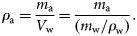
The density contrast (g) of P. pugio ranged from 0.873 to 1.155, with a mean and standard deviation (s.d.) of 1.020 ± 0.035 (n = 229; Table 1, Figure 1). The variability of the measurement technique for this species was <2.4%. This was calculated by taking the difference in the minimum and maximum density from the multiple measurements of each animal, then calculating the median value for all animals. As expected, the smallest animals had the greatest variability, but for most of our measurements, the uncertainty in our measurement technique is much less than the variability measured from different animals. Animal lengths ranged from 21 to 43 mm, and mean animal mass ranged from 0.069 to 0.731 g. Animal mass and volume were both positively correlated with animal length (y = 0.281 x − 0.594, r² = 0.89, and y = 0.260 x − 0.540, r² = 0.89, respectively). The greatest variation in g measurements was among those animals with a mass <0.3 g.

Figure 1.

Density contrast (g) measurements for shrimp, fish, and polychaetes species with respect to animal mass. The line represents g equal to 1, which is where the density of the animals is equal to the density of seawater. Density contrast (g) measurements for fed (filled circles) and starved (open circles) C. septemspinosa were significantly different (t-test, p = 0.006). Polychaetes showed a significant difference (Mann–Whitney rank-sum test, p = 0.018) between N. succinea (filled circles) and G. americana (plus). Note that median values were analysed for polychaete species because the dataset did not pass the equal variance test.

Table 1.

Density contrast (g) measurements for each of the groups of animals studied.

Animal group	n	Density contrast
		Min.	Max.	Mean ± s.d.	Median
P. pugiobc
All P. pugio	229	0.873	1.155	1.020 ± 0.035	1.028
Gravid	17	1.030	1.063	1.045 ± 0.009	1.040
Eggs removed	17	1.019	1.057	1.034 ± 0.010	1.034
C. septemspinosaab
All C. septemspinosa	105	0.870	1.085	0.990 ± 0.047	0.995
Fed	55	0.907	1.085	1.001 ± 0.048	1.006
Starved	43	0.870	1.051	0.975 ± 0.041	0.975
F. majalis
All F. majalis	60	0.958	1.023	0.996 ± 0.012	0.997
F. heteroclitusbd
All F. heteroclitus	48	0.942	1.030	0.999 ± 0.018	1.003
Males	10	0.993	1.016	1.001 ± 0.007	0.997
Females	29	0.984	1.030	1.005 ± 0.011	1.005
Juveniles	9	0.942	1.021	0.977 ± 0.028	0.982
Polychaetese
All polychaetes	53	0.915	1.066	1.006 ± 0.031	1.016
N. succinea	27	0.930	1.048	1.015 ± 0.022	1.017
G. americana	21	0.915	1.066	0.994 ± 0.037	1.000

Significant differences (p < 0.05) in animal density were related to the animals' feeding status (a), length (b), reproductive status (c), sex and maturity (d), or species (e).

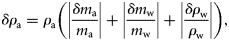
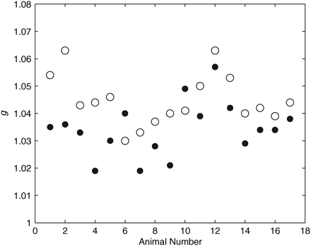
Palaemonetes pugio were separated into groups of 5 mm increments, and the median values were compared for trends in g. Median g increased with length, with the two larger groups (35–39 and 40–44 mm) being significantly larger (Kruskal–Wallis one-way ANOVA on ranks, p < 0.001) than the groups of smaller shrimp (20–24, 25–29, and 30–34 mm; Figure 2).

Figure 2.

Density contrast (g) measurements for shrimp and fish species with respect to animal length. The line represents g equal to 1, which is where the density of the animals is equal to the density of seawater. Density contrast (g) measurements for fed (filled circles) and starved (open circles) C. septemspinosa were significantly different (t-test, p = 0.006).

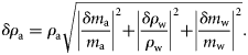
The mean g of P. pugio increased during the starvation experiment, with medians of 1.024 for shrimps that had been fed and 1.032 for those starved for 1 week; however, this difference was not significant (Mann–Whitney rank-sum test, p = 0.129, n = 229). The mean mass of P. pugio did not change significantly during the starvation experiment, although the mass of many animals did decrease. These averages are for a group of animals, not individuals, and the number of starved shrimp was typically less than the number of fed shrimp as a result of mortality. The effect of the presence of eggs on 17 gravid P. pugio was also tested. For 15 of the 17 P. pugio, g decreased after the eggs were removed (Figure 3). Mean g was significantly greater (paired t-test, p = 0.003) for gravid shrimps (mean g = 1.045) than for shrimps from which the eggs had been removed (mean g = 1.034). Accurate measurements of g were difficult to make for the eggs because of their small size (approximately tens of micrometres). Indirect measurements of egg density were calculated from the egg mass (equal to the mass of a gravid shrimp minus the mass of a barren shrimp) and the volume (equal to the volume of a gravid shrimp minus the volume of a barren shrimp), then used to calculate g (mean g = 1.107).

Figure 3.

Mean values of g for gravid (open circles) P. pugio and immediately after eggs were removed (filled circles; n = 17). There was a significant decrease in g after the eggs were removed (t-test, p < 0.001).

The salinity variation experiment showed no significant effects on g from the different salinity environments (one-way ANOVA, p = 0.367, n = 7). Palaemonetes pugio acclimated to 28 psu for 2 d had a mean g of 1.035 ± 0.009 (s.d.). Salinity was then increased to 35 psu for 2 d, resulting in a slight decrease in g (1.024 ± 0.016). When the salinity was lowered to 30 psu for 2 d, g increased to 1.037 ± 0.010, but then decreased to 1.030 ± 0.017 after acclimatation to 25 psu.

Crangon septemspinosa

The density contrast of C. septemspinosa ranged from 0.870 to 1.085, with a mean and s.d. of 0.990 ± 0.047 (n = 98; Table 1, Figure 1). The variability of the measurement technique for this species was <3.1%, the smallest animals having the greatest variability. Unlike P. pugio, there was a significant difference in g for the feeding treatments (t-test, p = 0.006). Mean g decreased from 1.001 ± 0.048 (n = 55) to 0.975 ± 0.041 (n = 43) after starvation for 1 week. There was no significant change in animal size (mean mass or length) during starvation.

Both mass and volume of C. septemspinosa were positively correlated with animal length (y = 0.198 x − 0.435, r² = 0.86, and y = 0.185 x − 0.395, r² = 0.86, respectively). Except for the largest group of C. septemspinosa (45–49 mm), the mean g increased as the length of shrimp increased (Figure 2). There were significant differences (one-way ANOVA, p < 0.001) between the length interval of 40–44 mm (mean g = 1.033) and both 20–24 mm (mean g = 0.953) and 30–34 mm (mean g = 0.984). There was also a significant difference in mean g between shrimps with lengths of 35–39 mm (mean g = 1.007) and those with lengths of 20–24 and 25–29 mm.

Fundulus majalis

Fundulus majalis had a mean g and s.d. of 0.996 ± 0.012 (n = 60), with a range of 0.958–1.023 (Table 1, Figure 1). The variability of the measurement technique for this species was <2.2%. Variations in animal physiology did not have a significant effect on the measurements of g. Mean g and s.d. decreased from 0.997 ± 0.012 to 0.995 ± 0.013 after the 1-week starvation period, but this difference was not significant (t-test, p = 0.460). The sex and maturity (male, female, and juvenile) of the fish also did not have a significant effect on the values of g. The mean g and s.d. of males was 0.994 ± 0.013 (n = 40) and of females 0.998 ± 0.012 (n = 18), whereas the mean g and s.d. of juveniles was 1.007 ± 0.013 (n = 2). Animal mass and volume were both positively correlated with the length of F. majalis (y = 1.959 x − 8.99, r² = 0.83, and y = 1.904 x − 8.723, r² = 0.86, respectively). There was no significant difference between the length of the animal and its material properties (Figure 2).

Fundulus heteroclitus

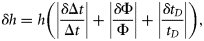
Fundulus heteroclitus were collected in autumn 2006 and spring 2007. The mean g and s.d. was 0.999 ± 0.018 (n = 48). The variability of the measurement technique for this species was <1.9%. Variability was greatest in the smaller fish, ranging from 0.942 to 1.030. Some 60% of the fish had a value of g < 1, whereas the remaining 40% had a value of g > 1 (Table 1, Figure 1). The lower range in g for F. heteroclitus was the result of two juveniles that were each measured twice, once after they had been fed and a second time after starvation. If measurements from these two fish were excluded, the range of values of g would have been closer to the range measured for zooplankton. A buoyancy test conducted on several anaesthetized fish confirmed that some fish had a greater density than seawater, whereas some were less dense (Figure 4). Relationships between length and mean g showed that specimens of F. heteroclitus with a length of 30–39 mm had a mean g (0.957) significantly less than each of the larger groups of fish (one-way ANOVA, p < 0.001; Figure 2). Animal mass and volume were both positively correlated with animal length (y = 1.594 x − 6.579, r² = 0.86, and y = 1.543 x − 6.350, r² = 0.86, respectively).

Figure 4.

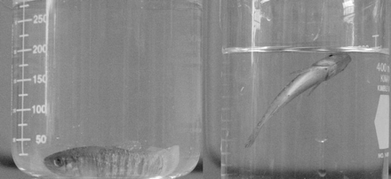
Fundulus heteroclitus were anaesthetized to restrict buoyancy control or active movements before being placed in a beaker of seawater to confirm our measurements of g. The fish to the left had a g >1, meaning it was denser than the seawater, whereas the fish to the right had a g <1, meaning it was less dense than seawater.

The material properties of F. heteroclitus were not affected by their nutritional status. Although the mean mass of the fish increased slightly during the week of starvation, so did mean g, although this increase was small and not significant. The effect of sex and maturity of the fish was also examined. Although males (median g = 1.005, n = 10) and females (median g = 0.982, n = 9) were not significantly different in terms of their values of g (Kruskal–Wallis one-way ANOVA on ranks, p = 0.015), there was a significant difference between females and juveniles (median g = 0.997, n = 29).

Polychaetes

In all, 31 polychaetes (N. succinea and G. americana) were collected for analysis. Measurements of g ranged from 0.915 to 1.066 with a mean and s.d. of 1.006 ± 0.031 (Table 1, Figure 1). The variability of the measurement technique for this species was <2.3%. Although there was a large range of values, each polychaete with a value of g < 1 had a mass of <1.3 g, most of them being <0.5 g. For animals with such a small mass, the accuracy and precision of measurements of g decreases.

The animals were then starved for a week. Only 17 were available for a second measurement. The comparison of the fed (median g = 1.015, n = 31) and starved (median g = 1.012, n = 17) polychaetes showed no significant difference (Mann–Whitney rank-sum test, p = 0.546). The two species of polychaete measured had mean values of g that differed significantly (Mann–Whitney rank-sum test, p = 0.018). The median g for N. succinea was 1.017, and that for G. americana was 1.000.

Sound-speed contrast

The sound-speed contrast (h) for the shrimps was <1. Palaemonetes pugio ranged from 0.9691 to 1.0000 with a mean and s.d. of 0.9953 ± 0.0082 (n = 14; Table 2). The range of measurements of h for C. septemspinosa was from 0.8721 to 1.000, with a mean and s.d. of 0.9737 ± 0.0457 (n = 7; Table 2). There was a greater range of h for the fish, with half the measurements for each species >1 and the other half <1. The range of measurements of h for F. majalis was 0.8977–1.1410, with a mean and s.d. of 1.0196 ± 0.0782 (n = 10; Table 2). Fundulus heteroclitus had a range of values of h of 0.9682–1.1410, with a mean and s.d. of 1.0245 ± 0.0609 (n = 7; Table 2). The polychaete range of h values was 0.9878–1.0440, with a mean and s.d. of 1.0023 ± 0.0163 (n = 8; Table 2). The volume fractions for these measurements varied as a consequence of the difference in animal morphology and the number of animals available for the experiment. The range was from ∼5 to 90%, with most measurements with volume fractions greater than one-third (Φ > 33%).

Table 2.

Sound-speed contrast (h) measurements for each of the groups of animals studied.

Animal group	Sound-speed contrast
	Min.	Max.	Mean ± s.d.
P. pugio	0.9691	1.0000	0.9953 ± 0.0082
C. septemspinosa	0.8721	1.0000	0.9734 ± 0.0457
F. majalis	0.8977	1.1410	1.0196 ± 0.0782
F. heteroclitus	0.9682	1.1410	1.0245 ± 0.0609
Polychaetes	0.9878	1.0440	1.0023 ± 0.0163

Calculating TS

The TS of a fluid-like crustacean was calculated for nine different combinations of values using the upper and lower range and means of g and h for P. pugio at frequencies of 38, 120, and 200 kHz. A change in g had the biggest effect on the TS of the animals. The TS calculated from the mean g (1.020) was substantially less than when calculated from the upper and lower range of values. As g moves closer to 1, the TS decreases because the density of the animal is closer to the density of seawater, less sound is scattered, and the animals have a lower TS (Figure 5). The lower the TS calculated, the larger the animal's estimated abundance. Variations in animal abundance of up to three orders of magnitude were calculated when the model inputs g and h were varied over the range of measurements made here (Table 3).

Figure 5.

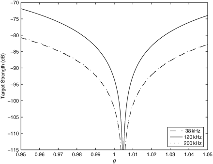
The TS of a 3.5-cm long animal at frequencies of 38, 120, and 200 kHz decreases as g approaches unity. The TS values for 120 and 200 kHz are very similar, so the lines overlap. The TS was calculated using Equation (7) from Stanton and Chu (2000). The sound-speed contrast (h) value used was the mean value calculated for P. pugio (0.9953).

Table 3.

Animal abundance estimates (n) vary greatly depending on whether minimum, mean, or maximum values of material properties are used as inputs into acoustic scattering models.

g	h	38 kHz		120 kHz		200 kHz
		TS	n	TS	n	TS	n
0.873	0.9691	−71.4	44	−63.1	6	−71.2	42
0.873	0.9953	−73.4	68	−64.5	9	−73.2	66
0.873	1.0000	−73.7	75	−64.8	9	−73.5	72
1.020	0.9691	−93.9	7 807	−85.6	1 141	−93.8	7 516
1.020	0.9953	−92.1	5 082	−83.2	658	−91.9	4 931
1.020	1.0000	−89.8	3 010	−80.8	381	−89.6	2 884
1.155	0.9691	−73.6	73	−65.3	11	−73.5	70
1.155	0.9953	−72.2	53	−63.3	7	−72.1	51
1.155	1.0000	−72.0	50	−63.0	6	−71.8	48

Density and sound-speed contrasts (g and h, respectively) were used to calculate the TS of P. pugio at frequencies of 38, 120, and 200 kHz (using a scattering model from Stanton and Chu, 2000). The values of g and h were chosen because they are either the mean or the upper and lower bounds of the range for P. pugio in this study. The TS was then used to calculate the number of animals (n, rounded to the nearest integer) present in a volume of water with an S_v equal to −55 dB.

Discussion

Knowledge of the material properties of marine organisms is necessary for accurate calculation of abundance or biomass from acoustic survey data. The density (g) and sound-speed (h) contrasts are two important variables necessary to make these calculations. Previous studies have used constant values of g and h for a species, but it is clearly better to investigate whether the physiological or environmental conditions influence these values and what would be the implications of varying estimates of abundance or biomass. Physiological conditions that were investigated were the organism's health (fed vs. starved), size (length and mass), reproductive status, sex, and maturity. The effects of environmental conditions, such as salinity and density of seawater, on g were also examined.

Each group of animals studied had a mean g within the range of values observed previously for zooplankton (0.9862–1.0622; Chu et al., 2000a). The range of measurements, however, exceeded previously published values. There was a great variability in the values of g measured, with the most variability among individuals of small mass. For example, the greatest variability for P. pugio was for those with a mass <0.3 g. A source of error when using the volume displacement method is interstitial water remaining on the animal. Although the mass of one drop of water is very small, it can have a large effect when calculating the density of animals with small mass. This can also explain the great variability found for C. septemspinosa, which were only collected in winter and early spring when they tend to be smaller. There was also a large range in g for polychaetes, but most of the variability was confined to the smaller G. americana. All polychaetes with a value of g < 1 had a mass <1.3 g, and most were <0.5 g.

There was no significant difference between feeding treatments for either fish species or the polychaetes. However, there was a significant difference for the shrimps. The difference in g for the different feeding treatments for P. pugio was not significant; however, when individuals with a mass <0.3 g were excluded, the starved shrimp were significantly more dense than the fed shrimp (t-test, p = 0.035). This increase in density may be the result of the consumption of the less dense lipid reserves (Campbell and Dower, 2003) during starvation. The opposite effect was manifest when C. septemspinosa were starved, resulting in a significant decrease in mean g.

The effect of sex and maturity on g was also studied for both species of Fundulus. There was no significant difference in g between male, female, and juvenile F. majalis. There was no significant difference in mean g between male and female F. heteroclitus, but juveniles had a mean g significantly less than females. This difference may be the result of physiological changes as the fish develop into adults. The effect of the reproductive status on the measurements of g for P. pugio was investigated. Gravid P. pugio had a significantly higher g than when their eggs had been removed. The gravid state is energetically costly, causing depletion of lipid reserves (Evanson et al., 2000; Lundberg et al., 2006), which would normally decrease the density of the animal. However, the density of eggs may be so high that the density of a shrimp carrying eggs increases (Salzen, 1956).

Except F. heteroclitus, animal size resulted in significant differences in g. Trends were for an increase in g with animal length, supporting the results of earlier studies (Chu and Wiebe, 2005; Lawson et al., 2006) that demonstrated a correlation between the length of the animal and g.

An experiment looking at the change in g as P. pugio were acclimated to salinity that was increased and decreased demonstrated no significant changes. As animals that live in estuarine environments, they are faced with salinity fluctuation as the tide changes, making it necessary to withstand changes over a short period without major physiological adaptation. An acclimation period of just 2 d may not have been sufficient to result in physiological change from acclimating to different environmental conditions. Another possibility is that the animals adjusted rapidly to their new environment but were able to maintain a relatively constant density ratio.

The fish and polychaetes had a mean h between the range of values typically used for zooplankton (0.9978–1.0353; Chu et al., 2000a), but both species of shrimp had a mean h less than this. The sound-speed contrast (h) was not affected by physiological and environmental conditions for any of the species studied. As a sound wave travels from one medium to another, its speed will alter. It is predicted that the speed of a sound wave passing into a denser medium will increase (Marczak, 1997). This assumption was confirmed with h measurements calculated on both F. heteroclitus and polychaetes, whose mean g and h were both slightly >1. On the other hand, the speed of sound is predicted to decrease as a sound wave travels to a less dense medium, as seen for C. septemspinosa, which had a mean g of <1. An exception to this assumption was found for P. pugio, which had a mean g of >1, but a mean h of <1, and F. majalis, which had a mean g of <1 and a mean h of > 1.

Acoustic surveys measure the sound scattered by targets in the water column, and the TS of the scattering animals is used to translate this information into abundance or biomass estimates. Constant values for g and h are typically used to calculate TS. For example, the widely used values (Everson et al., 1990; Stanton et al., 1998b; Stanton and Chu, 2000) found by Foote et al. (1990) for Euphausia superba have g equal to 1.0357 and h equal to 1.0279. However, the g and h measurements made here show that a single value may not be appropriate to describe a species. It may be important instead to look at a range of values rather than just a mean value. The TS of P. pugio calculated from the mean g was significantly lower than when the upper and lower ranges were used. As g moves closer to 1, less sound will scatter, giving a TS that results in two, or even three, orders of magnitude difference in abundance estimates. Using one value for g and h, calculations of biomass and abundance will therefore be susceptible to either over- or underestimation if they are not accurate for the population being investigated. As has been done with the length parameter in acoustic modelling (Lawson et al., 2006), it may be necessary to use a distribution function or a range of values for g and h.

Both trawl and acoustic survey methods do have limitations, but if these limitations are understood, they can be used effectively to estimate abundance or biomass. The variability in abundance from net tows is a result of zooplankton patchiness, and the variability in acoustic abundance estimates using a constant value for g and h is a systematic or methodological artefact. These inaccuracies in abundance estimates will be consistent during a study.

Current scattering models often assume constant values of g and h, but we know that these parameters are a function of body composition and will vary from animal to animal, and even within an animal. Therefore, the animal's physiology, such as lipid content, muscle tissue, organs, and gonads, will likely affect its material properties. It may be important to use a range of values of scattering model inputs to provide an upper and lower bound for abundance estimates. In order for acoustics to become a more accurate sampling technique for assessing animal abundance, the material properties of ecologically important zooplankton need to be better studied so that the accuracy of scattering models can be improved.

Acknowledgements

We gratefully acknowledge the assistance of the Stony Brook University Southampton Marine Station, particularly Melanie Meade. Libby Beckman, Kestrel Perez, Masatoshi Sugeno, and Konstantine Rountos assisted with sample collection. Bradley Peterson assisted with statistical calculations. The work was supported in part by the National Science Foundation, Grant No. OPP-06-33939. This is contribution 1384 of the Marine Sciences Research Center at Stony Brook University.