The eastern Baltic cod fishery: a fleet-based management strategy evaluation framework to assess the cod recovery plan of 2008

Abstract

Bastardie, F., Nielsen, J. R., and Kraus, G. 2010. The eastern Baltic cod fishery: a fleet-based management strategy evaluation framework to assess the cod recovery plan of 2008. – ICES Journal of Marine Science, 67: 71–86.

A management strategy evaluation framework was developed for the international Baltic cod fishery to evaluate the performance and robustness of the 2008 multi-annual management plan for the eastern stock. The spatially explicit management evaluation covered two cod recruitment regimes and various fleet adaptation scenarios. The tested management options included total allowable catch control, direct effort control, and closed areas and seasons. The modelled fleet responded to management by misreporting, improving catching power, adapting capacity, and reallocating fishing effort. The model was calibrated with spatially and temporally disaggregated landings and effort data from five countries covering 83% of the total cod catches. The simulations revealed that the management plan is robust and likely to rebuild the stock in the medium term even under low recruitment. Direct effort reduction limited underreporting of catches, but the overall effect was impaired by the increased catching power or spatio-temporal effort reallocation. Closures had a positive effect, protecting part of the population from being caught, but the effect was impaired if there was seasonal effort reallocation. Over the entire 15-year simulation period, all fleets could realize variable but positive profits under all scenarios tested, owing to stock recovery.

Introduction

The eastern Baltic cod (Gadus morhua) stock has recovered slowly from extremely low levels to safe biological limits (ICES, 2009). A long-term recovery plan was introduced in 2008 to bring the stock back to precautionary levels (EC, 2007). Earlier management failed to produce significant stock recovery, partly because the regulations led to unintended responses of the fishery in compensating for the reduction in fishing pressure (ICES, 2008a). For example, non-compliance in the form of misreporting of landings (ICES, 2008a) introduced uncertainty and bias into the stock assessments and, hence, to the precautionary reference points, and impaired the effectiveness of management in general. Moreover, a regime shift driven by a change in Atlantic water inflow frequency and intensity into the Baltic Proper in the early 1990s (Alheit et al., 2005) created adverse conditions for cod reproduction and exacerbated the poor performance of the existing regulations in rebuilding the cod population.

The multi-annual management plan introduced in 2008 is one of the first implemented to combine total allowable catch (TAC) and effort control management systems within the European Common Fisheries Policy. TAC and total allowable effort (TAE) are set corresponding to a gradual reduction in fishing mortality, F, by 10% per year until the stock recovers to the targeted F at 0.3 (EC, 2007). The decision rules of the plan, as well as the conversion of the F reduction into TAC and effort E, are depicted in Figure 1. The rationale behind the plan was to guide stakeholders with concise decision rules that are consistent with the management objectives and indexed on the most recently assessed F. Additionally, indirect effort controls through periodic fishing closures have been maintained in the 2008 recovery plan (EC, 2005; Nielsen et al., 2006) combined with technical measures (e.g. gear and mesh-size regulations) and more stringent fishing effort controls (since 2007).

Figure 1.

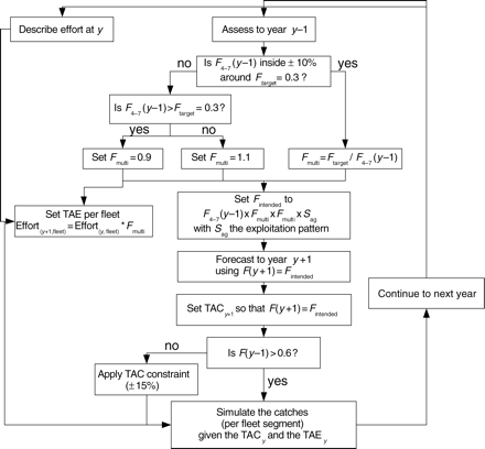
Overview of the model of the Baltic cod management plan.

The past 10–15 years have seen frequent changes in the management of the Baltic cod fisheries, with various types of regulation implemented in parallel or changing from one year to the next. The effect of each measure individually is difficult to evaluate. Therefore, we developed a spatially explicit bioeconomic model for management strategy evaluation (MSE) to reveal the effects of management scenarios on stocks and fisheries from both biological and economic perspectives. Existing knowledge and new analyses of recent historical developments in stocks and fisheries were combined in the model. The model framework allowed for testing management options in a multifleet context, including the evaluation of robustness towards changing fishing patterns resulting from the adaptive behaviour of fishers. The model computed profit from area- and season-disaggregated revenue on an array of species minus the costs of fishing to evaluate the direct economic effects for each fleet. As such, the model allowed for the evaluation of behavioural responses from the groups of fishers to regulations or changes in resource availability.

The relative performance and robustness of TAC vs. TAE management systems was investigated for different scenarios of (i) environmental conditions affecting cod recruitment, and (ii) presumed fleet adaptations. Behavioural side effects of changes in management regimes such as non-compliance, efficiency improvement, capacity adjustment, and redistribution of E in space and time are addressed in the study.

Material and methods

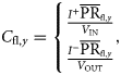
The simulation framework consists of three elements: the operating model (OM), the observation-error model (OEM), and the management procedure (MP; Rademeyer et al., 2007). The OM simulates population and fleet dynamics and represents alternative plausible hypotheses about stock and fishery, allowing the integration of higher level complexity and knowledge than generally possible within stock assessments. The OEM describes how simulated fisheries data are sampled from the OM, and the MP or management strategy is the combination of the simulated data, the stock status derived from an assessment of the simulated stock, and the management model or harvest control rule (HCR) that generates the setting of management measures, such as a target rate of F, a TAC, or a TAE. In the present application, the MP examines TAC management, direct effort control, or closed fishing areas and seasons. An important aspect of MSE is that management measures are cycled back into the OM so that their impact is reflected in the simulated stock and fishery. The simulation framework was developed in R (R Development Core Team, 2007) using the FLR platform [Fisheries libraries in R; www.flr-project.org; Kell et al. (2007); www.efimas.org], a software toolbox for fisheries modelling.

The operating model

The relationship between the spatially disaggregated E and the resulting F is the core of the OM, linking the population dynamics and the fishery. A linear relationship is assumed:

1

The dimensions are fl for a fleet segment (i.e. a combination of a country co, a vessel category vc, and a gear component gr), ag for fish age, ar for area, and se for season. The catchability composite term, Q, quantifies factors other than fish availability (abundance), which can impact the catch rates:

2

q being a calibration factor, Sel the selectivity pattern, Pow the relative catching power of a given fleet segment, and Mis the misreporting factor. Therefore, the partial fishing mortalities F_fl,ag,se,ar incorporate differences between fleet segments in catching power, gear selectivity, and the spatio-temporal effort distribution, E_fl,se,ar, in days at sea. E_fl,se,ar is split as follows:

3

with CP being the initial total number of vessels participating in the fishery (capacity), which according to input data is subdivided into shares (fractions) of CO, the share of country co, VC the share of vessel category vc (length categories), and SE, the active vessel share, which depends on the season se dimension (not all vessels are active at all times). The effort shares are GR, the share of gear gr (effort per gear category), and AR, the share of area ar, introducing the spatial dimension. 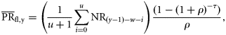Vessel activity is in days at sea and is the average nominal effort per vessel for a given fleet per month. AHF is a multiplication factor to scale the fleet capacity to investment/disinvestment dynamics (Hoff and Frost, 2008).

Each contribution from the different fleet segments is summed to obtain the spatially and seasonally disaggregated F:

4

The overall stock-specific F-at-age F_ag is obtained by removing the area and season dimensions and by summing over areas under the assumption of constant natural mortality, M:

5

N being the population abundance, then solving for F_se,ag:

6

and

7

F is reflected in stock dynamics through the classical exponential decay [Equation (8)] with A the plus group (age 8), M = 0.017 per month (M = 0.2 per year) for all fish ages:

8

if se is the last season of the year, or as follows if otherwise:

9

Using the Baranov equation (Baranov, 1948), catches including discards are computed from the seasonally and spatially disaggregated F. Total catches per area per season are then distributed between fleets according to their contribution to the total F to obtain spatial and seasonal information on catches and economy by fleet. The economic gross return GRR is computed from landings in numbers L (after subtraction of discards) using age-specific fish prices P and the fish weight W:

10

given the following price equation:

11

The α (baseline price) and β (price flexibility rate) are the parameters that account for a change in price depending on the total landings (Hoff and Frost, 2008). The net revenue NR, or profit, is computed from the (spatially disaggregated) gross return GRR minus the fishing costs. Costs cover variable and fixed costs; variable costs vary depending on vessel activity (e.g. fuel, ice, maintenance costs, crew share, sales costs), and fixed costs (e.g. rent of plant, insurance) are irrespective of activity. In the present context, costs per vessel are assumed to be average costs within each fleet segment:

12

where vcost1 and vcost2 are the variable cost functions in relation to E (e.g. fuel costs; costs per unit of effort) or revenue GRR (e.g. sales costs; a percentage of the catch revenue), respectively; fcost the fixed costs per vessel; CP the capacity (number of vessels); and VPUE the fleet-specific value per unit effort for not simulated species (e.g. flounder, herring, and sprat) caught in the Baltic fisheries.

Management procedure

The main steps of the procedure, i.e. the stock assessment, the HCR, the short-term forecast (STF), and the TAC settings are depicted in Figure 1. At the beginning of each year, y, a stock assessment is performed using extended survivor analysis (XSA; Shepherd, 1999), the method currently used by the ICES Baltic Fisheries Assessment Working Group (ICES, 2008a). XSA is a procedure for assessing the annual age-disaggregated F and abundance, N, in year y − 1 from the catch-at-age matrix, together with indices of abundance. As the catch per unit effort (cpue) abundance indices currently used in the ICES Working Group cannot be easily projected forward, the simulated abundance-at-age time-series was used for tuning. Some observation errors were assumed, both on the catch-at-age matrix and the age-specific abundance indices. These errors were drawn from the lognormal distributions with coefficients of variation (CVs) of 15 and 30%, respectively. The observation CVs were chosen according to the results from a stochastic multispecies model (Lewy and Vinther, 2004). Using the assessed mean F over ages 4–7, F_4–7, in year y − 1, the HCR was applied to decide on the mean intended F_y+1 for the coming year (Figure 1).

In the next step, a 2-year STF was performed (Figure 1), applying the F_y–1 and F_y to the assessed age-disaggregated N_y–1 and forecasted N_y, respectively, to obtain the forecast N_y+1 at age. F_y and F_y+1 are given by the mean F_4–7 in year y − 1 multiplied once and twice, respectively, by the F_multi (Figure 1) and disaggregated by age using the exploitation pattern of the previous years. This exploitation pattern S_ag was computed from the three previous years as follows:

13

In the STF, recruitment was set constant to the geometric mean over the past 17 years (ICES, 2008a). The TAC_y+1 in weight was computed as follows:

14

with the F_y+1 obtained from the HCR and the N_y+1,ag obtained from the STF, and W_ag the mean weight-at-age. Additionally, the TAC values were constrained by the HCR to remain within a given interval (±15% of the TAC in year y), so avoiding large annual fluctuations, except if F was >0.6 (Figure 1). The final TAC was calculated, removing the expected unofficial landings (ICES, 2008a), assuming the same level of misreporting across countries:

15

Finally, the TAC in weight was partitioned between participating countries to generate national quotas using the historical allocation key between Baltic countries. This is in agreement with the principle of relative stability as applied within the framework of the European Common Fisheries Policy (EC, 2001).

Effort-control management was modelled with TAE as the only control measure, or as a combination of TAE and TAC regulations, to determine the TAE for each year. The same procedure for assessing N and F in year y − 1 was used for the TAE system, and the HCR also decided on the F_multi (Figure 1). Then, the TAE in year y + 1 was calculated from the E in year y, applying the F_multi. The E reduction was directly proportional to the reduction of F by 10%, assuming a constant catchability Q, as found by Nielsen (2000) and Marchal et al. (2001) for the Baltic cod fishery. Further, it was assumed that there was neither misreporting of E nor an allocation key for distributing TAE between fleet segments. Rather, a homogeneous reduction (or increase) in the partial fleet E across fleet segments was considered, agreeing with the principle of relative stability.

Fleet adaptation

Scenarios of fleet adaptation behaviour (i.e. structured implementation error) have been evaluated under the TAC regime. It is assumed that when the TAC was exhausted for a given country, fleet segments continued fishing and started misreporting landings until the quota raised by a misreporting factor was exhausted. The misreporting factor Mis was kept constant, neglecting the possible effect of a fluctuating misreporting level, because the possible distribution of errors is too uncertain. In addition, an underreporting bias was possibly added, creating a systematic discrepancy of 10% between what had been decided by the managers and what had been caught. Long-term fleet capacity change caused by TAC fluctuations was simulated as exit–entry dynamics of vessels, which induced E reallocation between fisheries (Appendix).

Spatially and temporally explicit regulations were modelled specifying seasons, areas, years, and fleet segments affected by the regulations. If a regulation was enforced for a specific area and period in year y, the effort allocation in that area or season [AR and SE in Equation (3)] in year y − 1 was modified, so that E was removed from closed areas/seasons and entirely reallocated to the other possible fishing areas/seasons traditionally fished by the affected fleet segments. Plausible scenarios investigated at a short-term scale were (i) a closure-induced uniform spatial redistribution of E on all remaining open areas in which the fleet segment is known to operate, (ii) similar to (i) except that E is distributed proportionally to the relative area-specific cpue, and (iii) equal redistribution of E between the remaining open months in the given area.

In the scenarios of TAE regulation, induced E reallocation was simulated as follows: each year, the 10% effort cut was applied first to the area with the lowest cpue. Because of the lack of international data, short-term switching between demersal and pelagic gears targeting different species in the Baltic Sea could not be investigated. The effects of monotonic improvements in catching power were investigated by annually increasing the power (Pow) by 10% across fleet segments. In the simulations, no distinction was made depending on fleet segments, though in reality, smaller vessels or gillnetters are less likely to invest in new technology than large trawlers (Marchal et al., 2001).

Conditioning of the model to the eastern Baltic cod stock and fisheries

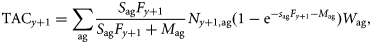
Spatial and temporal dimensions of the model were adjusted to the spatio-temporal regulations and to the resolution of available data, i.e. month and ICES statistical rectangle (time and spatial resolution for which logbook data are available). The fishery resource availability coefficients (Table 1) reflect the age-disaggregated cod abundance pattern over time and area and were obtained from analyses of the revised ICES Baltic International Trawl Survey data (Nielsen et al., 2001; ICES, 2007a). The decline in eastern Baltic cod over the years can partly be explained by a change in the abiotic conditions affecting cod reproductive success in the Baltic Sea (Alheit et al., 2005). Therefore, favourable and adverse environmental conditions for cod reproduction were identified. To predict recruitment R at age 2 in the OM, two segmented regression relationships for spawning-stock biomass against recruitment (SSB–R) were established for the periods 1966–1987 and 1988–2007, reflecting the periods of high and low recruitment of cod (Figure 2), respectively. Inflection points were set at SSB values of 250 000 and 85 000 t, respectively, based on visual inspection of the data. Errors on the recruitments were drawn from the longnormal distributions with CVs of 37 and 25%, respectively. Biological parameters for weight-at-age, the maturity ogive, and M were taken from ICES (2008a). The projected parameters are the arithmetic means over the years 2005–2007.

Figure 2.

Segmented regression for SSB–R relationships corresponding to high (grey line) and low recruitment (black line) regimes, using ICES data from the years 1966–1987 (squares) and 1988–2007 (black diamonds), respectively, with inflection points set at 250 000 and 85 000 t SSB, respectively.

Table 1.

Cod relative availability (%) by age in ICES Subdivisions 25–28 in the eastern Baltic, by semester and fish age.

Semester	ICES Subdivision	2	3	4	5	6	7	8+
1	25	59.69	58.66	66.30	57.69	46.38	42.08	39.09
	26	37.60	28.61	24.88	30.08	34.48	45.97	49.38
	27	0.16	1.02	0.58	0.26	0.21	0.00	0.00
	28	2.55	11.71	8.24	11.96	18.94	11.95	11.52
	All	100.00	100.00	100.00	100.00	100.00	100.00	100.00
2	25	76.65	41.78	80.97	81.68	91.58	77.91	79.36
	26	8.49	14.90	17.32	17.57	7.67	19.01	18.41
	27	0.00	0.00	0.02	0.00	0.00	0.00	0.00
	28	14.86	43.32	1.68	0.75	0.83	3.08	2.23
	All	100.00	100.00	100.00	100.00	100.00	100.00	100.00

The model was conditioned with catch-at-age and effort data from the international Baltic cod fishery (Denmark, Sweden, Latvia, Poland, and Germany) extracted from aggregated logbook, sales-slip, and vessel-register data. The model was initialized for 2003, the most recent year for which international data were available. Fleet segments were defined to minimize the computation demand as a combination of country, vessel size, and gear. Therefore, the 2003 landings and effort data were disaggregated by country, vessel size group, gear, area, and month. In all, 30 fleet segments were defined, i.e. five countries, three vessel size groups (<12, 12–24, >24 m), and four fishing gears (bottom trawls, pelagic trawls, gillnets, others). Relative catching power (Pow) per fleet segment [Equation (2)] was deduced by applying generalized linear models (Maunder and Punt, 2004) on cpue data (Table 2). Catching power indices were calculated relative to the catching power of a Danish trawl-fleet segment of medium vessel size chosen as reference. To avoid inconsistency between the simulated and the historical exploitation patterns, gear-specific selectivity ogives were not used. An overall ogive for selectivity Sel was deduced from the overall exploitation level given by the assessed F from the XSA. F-at-age was scaled to the maximal F over the 3 years before the start of projection. Gear-specific discard ogives played a minor role in our application because discards are mainly of cod aged 1 (FB, pers. obs.), whereas our population recruits at age 2. The discard ogive reflects the observed situation in 2003 and is assumed to be representative for the entire period covered. The calibration factor q [Equation (2)] was set at 0.00054, i.e. the factor that scaled the simulated landings in 2003 to the observed ones. Mis, the raising factor accounting for misreported landings and landings from other countries (Finland, Russia, Lithuania, and Estonia), was set at 1.77 based on estimates of the total landings in 2003 (ICES, 2008a).

Table 2.

Generalized linear model (GLM) estimates of standardized fishing power by fleet segment (log-linear model weighted by the numbers of days at sea; log(cpue) = fleet + quarter: Subdivision, SD) from 2003 logbook data.

Source	Group	Estimate	Standard error	z-value	Pr(>|z|)	Exp(estimate)
(Intercept)		6.73	0.00	7 479.40	0.00	839.655
Fleet	Denmark.1.G	−2.23	0.00	−1 474.73	0.00	0.108
	Denmark.1.other	−0.59	0.00	−205.11	0.00	0.555
	Denmark.2.G	−2.15	0.00	−1 229.50	0.00	0.117
	Denmark.2.other	0.22	0.00	86.82	0.00	1.244
	Denmark.2.PT	−1.19	0.00	−485.88	0.00	0.303
	Denmark.2.BT	0.00	0.00	0.00	0.00	1.000
	Germany.1.BT	−1.56	0.03	−57.27	0.00	0.210
	Germany.2.BT	0.52	0.00	407.01	0.00	1.683
	Germany.2.G	1.03	0.00	239.41	0.00	2.812
	Germany.2.PT	−0.95	0.01	−81.25	0.00	0.388
	Germany.3.BT	0.68	0.00	470.52	0.00	1.966
	Germany.3.PT	−1.39	0.03	−41.95	0.00	0.250
	Latvia.1.G	−1.52	0.07	−20.90	0.00	0.220
	Latvia.2.BT	−0.25	0.00	−188.57	0.00	0.775
	Latvia.2.G	−0.59	0.00	−721.77	0.00	0.554
	Latvia.2.other	−0.88	0.00	−200.38	0.00	0.415
	Latvia.2.PT	0.24	0.01	43.27	0.00	1.271
	Poland.1.BT	−0.92	0.02	−50.35	0.00	0.399
	Poland.1.G	−1.08	0.00	−908.81	0.00	0.341
	Poland.1.other	−0.63	0.00	−535.49	0.00	0.530
	Poland.2.BT	0.16	0.00	242.58	0.00	1.170
	Poland.2.G	−0.22	0.00	−300.36	0.00	0.804
	Poland.2.other	−0.27	0.00	−254.66	0.00	0.760
	Poland.2.PT	1.18	0.00	469.49	0.00	3.242
	Sweden.1.BT	−1.13	0.00	−341.11	0.00	0.322
	Sweden.1.G	−1.01	0.00	−1 210.40	0.00	0.363
	Sweden.1.other	−0.85	0.00	−635.47	0.00	0.428
	Sweden.2.BT	−0.06	0.00	−92.39	0.00	0.939
	Sweden.2.G	−0.23	0.00	−219.36	0.00	0.798
	Sweden.2.other	−0.17	0.00	−90.84	0.00	0.848
Quarter:SD	quarter1:SD25	0.09	0.00	111.33	0.00	1.091
	quarter2:SD25	−0.01	0.00	−17.32	0.00	0.986
	quarter3:SD25	0.00	0.00	−2.24	0.03	0.998
	quarter4:SD25	0.10	0.00	122.17	0.00	1.104
	quarter1:SD26	−0.23	0.00	−242.13	0.00	0.796
	quarter2:SD26	0.03	0.00	30.93	0.00	1.031
	quarter3:SD26	−0.06	0.00	−56.91	0.00	0.938
	quarter4:SD26	0.00	0.00	0.00	0.00	1.000

The “:” operator is interpreted as the interaction of all variables appearing in the term.

The cost structure of Danish fleet segments sharing a common activity was available from the Danish Institute of Food Economics (FOI; www.foi.life.ku.dk/English/Statistics/Fisheries). For the other countries, cost structure and dynamics were not available. Also, the numbers of vessels per fleet segment from other countries had to be estimated from the fleet-segment-specific E per month for those countries, applying the Danish vessel-specific monthly values of effort. As a next step, the cost structure from Denmark by vessel size was applied to all countries. Flexible fish prices per commercial category (EC, 1996) were used. The α and β parameters of the price model [Equation (11)] were deduced from non-linear fitting of the landings to price data per commercial category covering the years 2003–2006. Average monthly fish price fluctuated between 14 and 18 DKK kg⁻¹. The revenues computed for each international fleet segment reflected the total revenue because they were simulated with consideration of revenues from catches of other species usually caught in the eastern Baltic, assuming constant VPUE for other species.

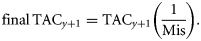
Closures as part of the management plan were mimicked in the simulations as closure A, the EC closure to protect spawning zones in ICES rectangles 40G5, 39G5, 38G5, 40G8, 39G9, and 38G9 (Figure 3), and closure B, a realistically sized seasonal closure of ICES Subdivisions 25–27. Both designs apply from 1 June to 30 September for all fishing activities.

Figure 3.

Fishery region with ICES Subdivisions (SD) and ICES statistical rectangles in the western (SD 22–24) and eastern Baltic (SD 25–32). The ICES rectangles corresponding to tested closures design A are shown in grey.

Simulation design

Simulation runs were split into two parts: (i) a historical part (2003–2007 inclusive) applying the stock dynamics, R, and F from the ICES (2008a) assessment used to validate the biological OM; and (ii) a projected part from 2008 on to 2015, applying the different MPs and the partial area-, season-, and age-disaggregated stock Fs computed from the fleet-specific fishing activities. If the TAC was in force, real catches in 2008 were set to 77 200 t, as suggested by ICES (2008b) in the STF, although the actual TAC was 42 300 t.

The performance of the management options tested was evaluated in terms of their relative capability to reach the predefined reference points for the eastern Baltic cod stock [limit reference point B_lim for SSB (B_lim = 160 000 t; STECF, 2006) and target F (F = 0.3; EC, 2007)]. The robustness to uncertainties was evaluated relatively and qualitatively among scenarios. An overview of all simulation scenarios performed is provided in Tables 3 and 4. In all, 100 iterations were carried out for each of the Table 3 scenarios, including closures. To evaluate the relative performance of different closures, the scenarios in Table 4 focused on the closure effect independently of the F reduction plan and the stochasticity on R, i.e. using constant recruitment. The business as usual (BAU) scenario corresponded to the situation with no management and E and F remaining at the 2008 level throughout the simulation. To limit our study, the choice of scenarios was based on preliminary simulation outputs. For example, if the plan was already able to rebuild the stock under a low-recruitment regime, it was considered worthless to simulate all combinations including a high-recruitment regime.

Table 3.

Tested combinations of management options, recruitment level, and fleet responses to the regulations (see text for abbreviations and detail).

Scenario	Management option	Recruitment level	Fleet adaptation
			Not fleet-specific	Fleet-specific
1	BAU	Low	–	–
2	BAU	High	–	–
3	TAC	Low	–	–
4	TAC	Low	–	Investment/disinvestment dynamics
5	TAC	Low	Underreporting	–
6	TAE	Low	–	–
7	TAE	Low	–	Directed effort reallocation
8	TAE	Low	10% efficiency increase	Directed effort reallocation
9	closure A	Low	–	Equal reallocation
10	closure A	Low	–	Directed reallocation
11	closure A	Low	–	Seasonal reallocation
12	TAE + TAC	Low	–	–
13	TAE + TAC	Low	10% efficiency increase	Directed effort reallocation
14	TAE + TAC	Low	Underreporting	–
15	TAE + closure A	Low	–	–
16	TAC + closure A	Low	–	–
17	TAE + TAC + closure A	Low	–	–
18	TAE + TAC + closure A	High	–	–
19	TAE + TAC + closure A	Low	Underreporting	Directed effort reallocation
			10% efficiency Increase

Table 4.

Tested scenarios evaluating closures without stochasticity on SSB–R, and without the F reduction plan.

Scenario	Management option	Recruitment level	Fleet adaptation
			Not fleet-specific	Fleet-specific
A	BAU	Low	–	–
B	BAU	High	–	–
C	Closure A	Low	–	Equal effort reallocation
D	Closure B	Low	–	Equal effort reallocation
E	Closure A	High	–	Equal effort reallocation
F	TAC	Low	–	–
G	TAC + closure A	Low	–	Equal effort reallocation

Results

In contrast to the BAU scenario of a high-recruitment regime (scenario 1), the stock was not able to recover under BAU with a low-recruitment regime (scenario 2), where the terminal SSB ranged from 50 000 to 75 000 t (Figure 4). None of the spatio-temporal closures (scenarios 9, 10, and 11) were able to reach management targets unless combined with TAC or direct effort control (scenarios 15–19). Notwithstanding, all closure designs led to increased SSB and landings in the medium term (Figure 5). Closing ICES Subdivisions 25–27 for 4 months each year under low recruitment (scenario D) led to an increase in SSB of ∼10 000 t and a gain in landings of 4000 t at the end of the simulation period. Under favourable recruitment, the SSB and landings increased strongly irrespective of the management scenario applied (Figures 4 and 5, Table 4). The positive effect of the extended closure on SSB was based on a short-term loss in total landings in the first 2 years, attributable to the closure (Figure 5). This loss could not be compensated during the closure when E was reallocated equally between the remaining open areas. Gains in landings during open periods were observed, but this surplus was not sufficient to balance the losses during the closure period (results not shown). The decrease in F resulting from the closure was mainly caused by the displacement of E into the western Baltic and the spatial change in the F pattern (scenario 9; Figure 6). Hence, more effort was applied in the open areas (owing to the redistribution of the same total effort), but on a lesser total abundance, leading to a lower overall F at the scale of a population. If effort was reallocated proportionally to previous years' cod cpue in open areas in the central Baltic (scenario 10), the increase in SSB was lower. Finally, when E was not displaced geographically, but instead redistributed to other seasons in the same area (scenario 11), the positive SSB effect diminished significantly as fleets compensated losses during other periods.

Figure 4.

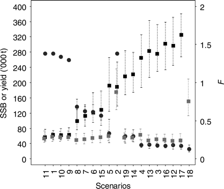
The 5% and 95% percentiles (n = 100 iterations for each scenario) for the final simulation year (2015) for SSB (median values shown by black squares), F_4–7 (median, black circles), and yield (median, grey squares) for different scenarios (Table 3). Scenarios are ordered according to the lower 5% limits for SSB. Note that the SSB for scenario 18 is out of range of the plot.

Figure 5.

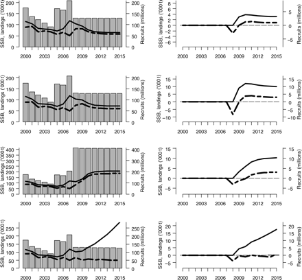
Simulated recruits (bars), landings (dashed line), and SSB (solid line) under a spatio-temporal closure and deterministic recruitment scenarios (Table 4), with the combinations from the top left to the bottom right being scenario C, scenario C relative to scenario A, scenario D, scenario D relative to scenario A, scenario E, scenario E relative to scenario B, scenario G, and scenario G relative to scenario F.

Figure 6.

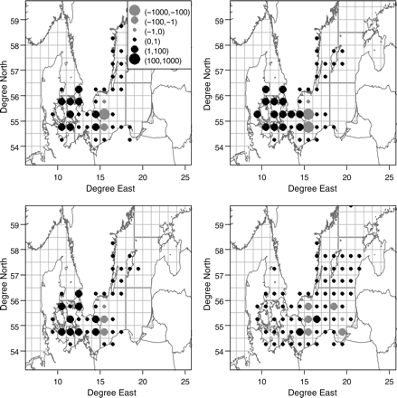
Effort distribution under scenario C in terms of gains or losses (in days at sea) relative to BAU (scenario A) during the closure period June–September in the final simulation year (black circle, gain in days at sea; grey circle, loss in days at sea).

In contrast to the BAU with a low-recruitment regime (scenario 1), the TAC system (scenario 3) led to stock recovery within 15 years (Figure 4). At the start of the period, the stock assessment underestimated SSB and overestimated F (Figure 7), because of the conservative model settings used (i.e. shrinkage procedure on F activated; see Kraak et al., 2008). Moreover, the MP computed STFs of biomass that were too pessimistic as a result of recruitment forecasts being underestimated (Figure 7). These forecasts led to a smaller TAC and targeted fishing mortality, F_y+1, resulting in significant reduction in F in 2009. This is allowed by the HCR when the last F assessed is >0.6. The TAC system performance was impaired, however, by systematic catch underreporting (scenario 5) of 10%, resulting in lower terminal SSB. The TAC system was also sensitive to a change in the number of active vessels when integrating the investment/disinvestment dynamics. When more fleets were free to invest in new vessels as a result of positive profits, this led to a lower final SSB level in 2015 (scenario 4) because there were some overquota catches.

Figure 7.

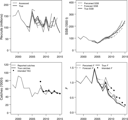
Simulated true (black) and perceived (grey) recruitment, SSB, catches, and F_4–7 for a single iteration of scenario 3, i.e. TAC management with low, stochastic recruitment.

Under the scenario of direct effort regulation with low recruitment (scenario 6), the continuous decrease in E driven by the HCR was not sufficient to reach B_lim and target F = 0.3 in most iterations. The probability of being below and above the respective targets was highest in the first part of the period (Figure 8a). This was mainly through the large increase in F at the start of the TAE period, when the fleets were able to catch more because there was no TAC constraining them (Figure 9). The more-or-less constant decrease in F in the final part of the period reflected continuous E reduction under a constant catchability assumption over the years because the management plan did not allow fluctuating E levels, in contrast to the TAC system.

Figure 8.

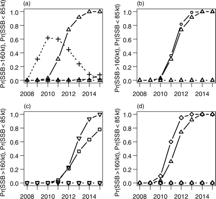
Probability that SSB is above B_lim (solid lines) or below the 85 000 t SSB–R inflection point (dotted lines). (a) TAE (cross; scenario 6) vs. TAC (triangle, scenario 3), (b) TAC + TAE (circle, scenario 12) vs. TAC (triangle, scenario 3), (c) TAC + 10% underreporting (square, scenario 5) vs. TAC + TAE + 10% underreporting (inverted triangle, scenario 9), and (d) TAC (triangle, scenario 3) vs. TAC + TAE + Closure A (diamond, scenario 17).

Figure 9.

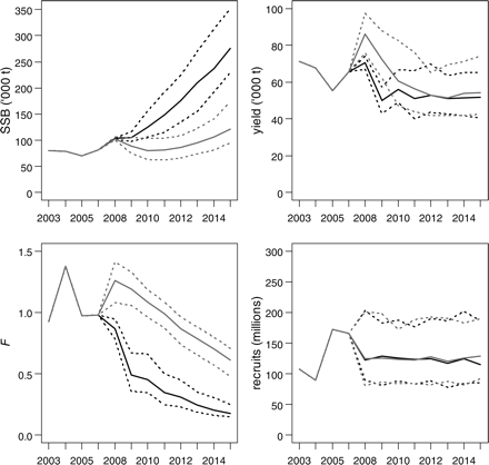
Simulated true SSB, yield, F_4–7, and recruits, comparing the TAC scenario (black, scenario 3) with the TAE scenario (grey, scenario 6). The medians are given as solid lines and the 5% and 95% percentiles as dotted lines.

Applying a combination of direct effort and TAC regulation (scenario 12), the recovery was faster and stronger than under TAC (scenario 3) or TAE (scenario 6) management alone, leading to a higher probability of attaining reference points (Figure 8b). The positive effect is partly explained by the lower catch levels than under the effort system without TAC restriction (Figure 9). Moreover, the reduction in E over the years reduced the impact of the observation errors because fleet-specific catch-quota exhaustion was sometimes prevented. The main effect of implementing the effort control combined with the TAC system was a decrease in the negative effect of underreporting (Figure 10). Final SSB under this scenario ranged from 175 000 to 279 000 t (scenario 14) compared with 125 000–266 000 t (scenario 12) and where the probability that SSB > B_lim was 1.00 vs. 0.75 (Figure 8c).

Figure 10.

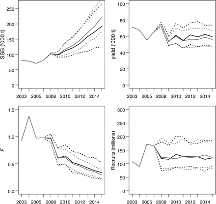
Simulated true SSB, yield, F_4–7, and recruits, comparing the TAC + 10% underreporting scenario (black, scenario 5) with the TAC + TAE + 10% underreporting scenario (grey, scenario 14).

The combination of TACs, direct effort control, and closures (scenario 17) provided the fastest stock recovery of all scenarios tested under the low-recruitment regime, with SSB ranging from 267 000 to 380 000 t at the end of the simulation period (Figure 4) and the probability that SSB > B_lim being 1 (Figure 8d). Performance of this scenario was impaired, however, if there was fleet adaptation (scenario 19), with SSB ranging from 168 000 to 283 000 t in 2015. If effort control was implemented without a TAC or closures (scenarios 6), fleet adaptation lowered the SSB in the final simulation year by 11% if the spatial reallocation depended on cpue (scenario 7). If this was combined with a 10% increase in fishing efficiency over the years (scenario 8), the loss in SSB increased to ∼20% in the final year (Figure 4).

With respect to economic consequences and performance, the Polish and Swedish fleets' final profits were higher under the TAE system than with a TAC or a TAC + TAE system, but the opposite was true for Danish fleets (Table 5; scenarios 6, 3, and 12, respectively). The TAC constrained the Swedish and Polish fleets more because they have greater capacity than Danish fleets and can catch more if only TAE is in force. The closure was therefore relatively more profitable for Danish fleets. No gear effect was found between scenarios unless the fleets were allowed to invest in new vessels (scenario 4). In that case, the capacity of Polish and Swedish trawlers increased and the profits of other fleets diminished (Table 5). Under the currently agreed management plan combining TAC, TAE, and indirect effort control through closures, fleet profits decreased significantly from 2008 to 2009 (Figure 11), especially for the Polish and Swedish fleets, whereas profit remained constant for the remaining simulation period when the TAC was almost constant. There was a slight profit increase attributable to the diminution of variable costs depending on effort (vcost1) along with effort reduction, together with an increase in cpue. Danish fleets were less impacted by the initial drop, because they were not able to exhaust their 2008 quota share given their effort and fleet catchability (not shown; ∼80% of the TAC was consumed).

Figure 11.

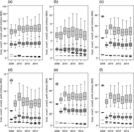
Scenario 17, bars indicating from dark to light: fcost, vcost1, vcost2, profit (i.e. NR, gross return from cod landings and other species minus the costs) in DKK (ICES SD 25). The depicted fleet segments are (a) 12–24 m Danish bottom trawlers, (b) <12 m Danish gillnetters, (c) 12–24 m Polish bottom trawlers, (d) <12 m Polish gillnetters, (e) 12–24 m Swedish bottom trawlers, and (f) <12 m Swedish gillnetters.

Table 5.

The 5%–95% percentiles of fleet-specific profit in the final year (2015) in million DKK for the main fleet segments for different combinations of management scenario (Table 3).

Scenario	Percentiles by fleet segment
	Denmark.2.BT	Denmark.1.G	Poland.2.BT	Poland.1.G	Sweden.2.BT	Sweden.1.G
1	36.4–57.0	2.3–5.4	49.9–74.4	6.2–10.4	43.1–68.7	20.3–33.2
2	111.8–203.6	13.8–27.7	140.3–249.4	21.4–39.8	137.0–251.4	66.6–123.2
3	49.8–97.8	5.1–20.1	40.3–65.2	3.5–9.1	37.7–65.8	13.3–25.1
4	57.7–97.2	−0.9–−15.2	28.4–64.3	0.0–2.03	51.5–92.3	4.8–10.2
5	66.1–107.4	7.1–18.8	46.3–74.1	5.3–10.9	43.2–70.1	16.6–29.6
6	36.1–66.8	4.8–9.7	47.9–85.0	7.4–13.7	48.8–87.8	22.8–41.7
7	33.1–60.0	4.42–8.3	44.3–75.3	6.78–12.11	45.01–77.6	20.3–37.2
8	31.7–58.5	4.1–8.3	42.9–74.3	6.42–11.9	43.1–76.5	20.1–36.7
9	34.4–53.5	1.7–3.5	55.5–82.0	7.3–11.8	48.9–76.4	23.0–36.3
10	35.0–57.1	1.4–3.3	52.7–81.4	6.5–11.2	44.5–73.3	21.0–35.3
11	38.1–66.5	0.5–3.6	46.3–76.6	5.8–10.7	40.3–71.8	18.7–34.2
12	52.7–92.5	8.7–17.7	35.7–62.3	4.1–8.7	34.7–63.7	13.6–26.6
13	53.1–88.1	9.7–17.9	36.1–61.4	4.35–8.8	36.9–62.7	13.4–26.3
14	61.4–95.7	9.2–17.2	46.3–69.2	6.6–11.4	45.0–66.7	19.1–30.7
15	30.5–58.2	2.2–4.8	50.8–91.5	8.0–15.1	51.8–94.4	23.9–44.6
16	65.9–104.5	1.7–6.5	40.9–68.1	3.3–8.5	41.9–70.2	13.5–24.9
17	61.0–106.3	2.7–8.5	36.3–67.2	3.9–9.3	37.2–67.9	14.1–28.3
18	178.4–324.0	4.7–19.7	116.5–223.6	9.1–25.9	117.4–268.5	36.5–82.3
19	65.3–108.8	3.8–8.2	43.4–78.8	5.6–12.2	44.4–74.4	17.4–32.1

Discussion

The aim of the present work was to provide a spatially explicit bioeconomic simulation tool to disentangle and anticipate the relative effects of different management options on the eastern Baltic cod stock and fisheries. The stock has been managed by a variety of frequently changing and overlapping regulations. The study was designed as an MSE that can identify management strategies robust to two major sources of uncertainty, (i) the environmental effect on cod recruitment success (process error), and (ii) the responses of fleets to regulations (implementation error). Observation errors (on input data required by the assessment model) have also been handled but kept constant, assuming that the actual errors remain in the same order of magnitude. Results of the simulations are evaluated against the capability of performance indicators, SSB and F, to reach B_lim and target levels for sustainability, as previously defined in other studies (STECF, 2006).

In relation to (i), the environmental conditions influencing cod recruitment proved to be a dominant factor in achieving biological sustainability. Even the BAU regime and, perhaps more pronounced, the plan combining TAE and TAC regulations were able to recover the stock quickly under favourable environmental conditions. All tested TAE without TAC scenarios (including closures) failed to recover the stock rapidly if the low-recruitment regime was applied. Although the assumption of constant adverse environmental conditions within the given time-horizon may be overly pessimistic, the environmental regime shift in the Baltic Sea associated with low recruitment in recent years implies that long periods of stagnation with adverse conditions for cod reproduction may not be exceptional in future (MacKenzie et al., 2007). Therefore, it is necessary to develop reliable environmental indicators for cod recruitment in relation to fisheries management and to investigate how these can be incorporated most efficiently into the advisory process. An environmental change in the Baltic Sea (Alheit et al., 2005) may create an incorrect perception of Baltic cod stock dynamics and lead to incorrect setting of management targets and precautionary limits for the stock. For instance, a B_lim set at 160 000 t does not appear to be sufficient for the stock to support long-term recovery and increasing fishing activity, as recently demonstrated by Köster et al. (2009).

In relation to (ii) above, the misreporting of catches and illegal landings is emphasized as a critical factor by the European Commission for regulation success (EC, 2007). However, the TAC under the management plan was not very sensitive to systematic underreporting of the catch. Underreported catch did not lead to very different trajectories towards the final stock biomass level over the years. If the high level of non-compliance estimated until recently (ICES, 2008a) made the success of the previous TAC management weaker, the TAC system should not be sensitive to misreporting provided a gradual F reduction was applied. Owing to a lack of data, however, incentives to misreport catches according to differences between fleets, TAC levels, or economic fleet profit levels were not simulated.

Although effort control has several advantages, better performance was demonstrated for a TAC system. Effort control is (i) simpler, avoiding the need for accurate short-term prediction, because only the assessed F in the previous year was used as a signal to decide on the next level of E, (ii) strongly coercive, i.e. by never allowing an increase in (nominal) E, and (iii) assumes no misreporting on E as an effect of an efficient fishery control and enforcement system, with more-intensive at-sea effort monitoring using satellite surveillance information. Moreover, because fishers are allowed to land and sell all legal-sized fish caught under an effort system, the incentive to misreport is low. Relaxing the catch constraint, effort control led, however, to higher catches than expected and put the stock at risk. Therefore, an agreed management plan that included a TAC system supplemented with effort control was the best combination. By a synergic effect, effort regulation increased the robustness of the TAC system in achieving management objectives.

The limited robustness of the effort-control system against fleet responses mitigated the positive effect of effort reduction on the TAC. For example, the effort system is sensitive to changes in catching power over time. In our model, the fleets reduced their E first in areas where cpue values were historically low. This led to a change in spatial fishing patterns when total E was reduced. Our stock projections demonstrated consequently that effort reduction should not be implemented alone, but rather along with a TAC system. Effort reduction needs to ensure that fleets do not catch more than expected, i.e. the robustness of the direct effort-reduction system is strongly dependent on the assumption of a constant exploitation pattern. This assumption is likely to be violated in a TAE system, particularly if effort is managed in days at sea (nominal E). If the total allowed days at sea is the most practical way to implement and enforce an effort system rather than other effort indicators such as engine power (Shepherd, 2003), management needs to take account of possible changes in the exploitation pattern.

The stock-based approach mainly conducted in EU fishery management uses an overall F deduced from an indivisible contribution of all fishery actors (Wilen et al., 2002). In some cases, poor performance of the stock-based approach for sustainable stock management led to us questioning the underlying assumptions of constant exploitation patterns. For example, when including the so-called technological creeping effect (the race for fish, with increasing engine power) into the simulations, the simulated SSB was lower and stock recovery was delayed. The efficiency of effort (nominal E) reduction was impaired when fleets became increasingly efficient, allowing a higher catch without a change in nominal E. Evaluation of a changing exploitation pattern in a realistic way requires the design of a multifleet dynamic model with fleet-based scenarios and spatio-temporal effort reallocation scenarios on a fleet basis. Fleet-based management allows resource management authorities to focus on fishing fleets, including the often neglected economic dimension of fisheries. In our model, fishing activity is analysed as a set of individual economic actors, including heterogeneous economic expectations and priorities. Here, the total stock-specific F is decomposed into partial Fs by country, set of vessels, or fleet segments, i.e. entities with a bioeconomic meaning and specific features such as geographic range of operation, fishing power, and effort-allocation behaviour. As the cod stock is shared between several coastal states in the Baltic, our level of complexity reflects the heterogeneity between the fishing actors and fleets. The decomposition of catchability linking E to F is essential, knowing that the control variable for managers is E and not directly the annual F.

Usually, the implementation error of a management plan can be added into an MP, but the structure of this error is certainly not simple. Indeed, fleet partial Fs fluctuate over time (and space) when fishing actors opportunistically change fishing activities, e.g. by targeting other species, or sometimes choosing to leave the fishery. In relation to the latter, some simulated fleet segments will choose to invest (and others to disinvest) based on their past profits, resulting in capacity redistribution inside the fishery and fleets. The exit of vessels from a fishery is likely under both TAC and TAE systems under continuous stock decline because the E allowed per vessel is reducing continuously along with individual profitability. The particular case of the Baltic cod recovery plan makes a homogeneous reduction in nominal E across countries and fleets likely because it has been assumed in the present simulations. However, our fleet-based economic evaluation demonstrated that fleets were still able to make a profit, whereas effort and catch quota were being reduced, because the stock was recovering during the period projected. The risk of recapitalization in the fishery from possible new entrants as a consequence of some vessels leaving or stock recovery should also be avoided if a closed licensing system for fishing rights on Baltic cod is maintained.

Fishing closures aim to modify the spatial fishing pattern to protect certain life stages of a stock from fishing. The closure effect is generally explained in the literature by enhanced recruitment from protected SSB (Botsford et al., 2007). The closure effect demonstrated here constituted a minimal expected effect. This is because recruitment was not indexed on SSB, the simulated recruitments (low or high) being kept constant when SSB was higher than the regression inflection points. This assumption has been established in agreement with a recent study on Baltic cod (Köster et al., 2005) which seems to reject the hypothesis that recruitment depends on SSB. Recruitment might rather be related to the magnitude and quality of reproductive volume, i.e. the volume of water that allows for successful egg survival and larva development (Nissling et al., 1994; Köster et al., 2005; MacKenzie et al., 2007). Species interactions could also be a driver for variations in recruitment (Van Leeuwen et al., 2008). The modular structure of our model allows extension of the biological OM with updated data, in particular using a foodweb model rather than the present single-species approach.

The closure effect shown in our simulations can be attributed only to a change in effort allocation. Therefore, it is imperative to take into account the space and time conjunction of the fleet activities along the spatially and temporally structured life cycle of stocks. When assuming complete compliance of fishers to closures, the simulated closure designs prevented a part of the stock being caught, and the biomass surplus was not totally harvested via spatial E reallocation. In contrast, the relatively small closure effect was not robust to a seasonal change in E because the closure effect vanished if E was redistributed to the remaining open periods. Closed areas exported fish to opened areas where they could be fished later. Moreover, the positive closure effect might be balanced out if fleets chose to increase their E to meet increased fishing costs. That scenario would be possible under a TAC-regulated fishery, but combination with direct effort control could eventually prevent this. Overall, closure performance was too poor to be an effective management tool for a stock where recruitment is not strongly related to SSB and exhibits distinct seasonal migrations. The magnitude of a closure effect also likely depends on the extension of the stock distribution area and related changes in spatial abundance, e.g. depending on environmental forcing and/or individual behaviour.

Investigation of the spatial dimension of a fishery could be of particular importance when harvested populations overlap. In this context, an effort control system has often been criticized because effort restriction is frequently based on catches of one stock (ICES, 2008b). As a result of bycatch (and discarding) or a change in target species according to fishing areas or seasons, other stocks could be overexploited in a mixed fishery. In our particular case, for example, closures led to effort being reallocated into the western Baltic, i.e. targeting a different stock. Effort reallocation towards western Baltic cod would have a major impact on that stock. Uncontrolled effort reallocation between stocks is likely under a pure, direct effort system (e.g. if no area restriction for deploying effort is defined). Therefore, the agreed management plan maintaining catch restriction per stock per area likely prevents fleets from fishing close to their designated harbours. These implications should be investigated further in a multispecies implementation of the model.

Effort-reallocation scenarios dependent on cpue have been tested. The profit that fleets expect from open fishing areas could likely drive E reallocation to a higher degree rather than cpue criteria alone (Hilborn, 2007). In that case, sophisticated decision choice models such as random utility models (Holland and Sutinen, 1999; Salas and Gaertner, 2004) may be methods of choice to redistribute the E based on, for example, knowledge of vessel-based cost structures. Different responses to the same regulation may also exist, and groups of fishers might be identified based on economic or social behaviour (Castillo and Saysel, 2005; Christensen and Raakjær, 2006). It should be emphasized that skippers' behaviours differ, and their responses to management measures may also differ. Coherent ways need to be found to capture those differences (Nielsen et al., 2006). Unfortunately, cost-structure data and dynamics per fleet are by nature difficult to obtain owing to their confidentiality and could not be obtained for countries other than Denmark for this study. Testing for a heterogeneous response would also require socio-economic data, which were similarly not available for this study.

Bioeconomic data have been used and simulated in the present study to evaluate short- and long-term reallocation effects on stock development, in response to regulations depending on spatially explicit and heterogeneous fleet-specific economic features. Further, the model can comprehend economically determined fleet capacity change through investment/disinvestment dynamics (see Appendix). The model can support such bioeconomic analysis of management regimes based on economic indicators to evaluate the capacity of regulations to drive multifleet fishing activity and capacity towards individual and/or global socio-economic targets. In addition, the model can act as a support for integrating fishers' decision-choice models in deciding on effort (re)allocation between fleets, species, areas, and seasons in response to regulations and/or change in stock availability.

Acknowledgements

The work was conducted through cooperation between the EU FP6 projects EFIMAS, CEVIS, and UNCOVER, and the Danish National DFFE Sustainability Package Project (Effort Regulation in the Baltic Sea), Danish Ministry of Food, Agriculture and Fishery. The findings do not necessarily reflect their views and in no way anticipates European Commission and Ministry future policy in the area. We thank Sarah Kraak, Coby Needle, and an anonymous reviewer for their suggestions for improvements to the manuscript, and Per Sparre, Keith Brander, Hans Lassen, Ayoe Hoff, and Hans Frost for valued comments. Funding to pay the Open Access publication charges for this article was provided by the Femern Belt project.

Appendix

The AHF model (Hoff and Frost, 2008) suggests a function to model capacity change via investment/disinvestment dynamics, which is used in the present model in a simplified manner. The capacity of a fleet is adjusted according to an investment decision function at an annual time-scale at the beginning of a year. The capacity change in the current year, taking w years (investment decision lag; w = 1) before the current year, is a function of the projected average profit PR through u + 1 years (i.e. the number of years on which investment decision is based, u = 2), which is given by

A1

with the right second term being the discounting of the average future revenues, NR the net revenue, ρ the interest rate (ρ = 0.05), τ the expected lifetime of a vessel (τ = 20), and the subscripts being y for year and fl for fleet. The investment decision function to model the change in capacity C is given by

A2

with I⁺ and I⁻ constituting parts of the profit dedicated to investment or disinvestment, respectively, and V_IN and V_OUT being the price of entry (i.e. price for a new vessel depending on the vessel category vc; vc1 = 758, vc2 = 1259, vc3 = 10 206 in '000 DKK) and exit (V_OUT = V_IN × 1.25), respectively.