Investigating agreement between different data sources using Bayesian state-space models: an application to estimating NE Atlantic mackerel catch and stock abundance

Abstract

Simmonds, E. J., Portilla, E., Skagen, D., Beare, D., and Reid, D. G. 2010. Investigating agreement between different data sources using Bayesian state-space models: an application to estimating NE Atlantic mackerel catch and stock abundance. – ICES Journal of Marine Science, 67: 1138–1153.

Bayesian Markov chain Monte Carlo methods are ideally suited to analyses of situations where there are a variety of data sources, particularly where the uncertainties differ markedly among the data and the estimated parameters can be correlated. The example of Northeast Atlantic (NEA) mackerel is used to evaluate the agreement between available data from egg surveys, tagging, and catch-at-age using multiple models within the Bayesian framework WINBUGS. The errors in each source of information are dealt with independently, and there is extensive exploration of potential sources of uncertainty in both the data and the model. Model options include variation by age and over time of both selectivity in the fishery and natural mortality, varying the precision and calculation method for spawning-stock biomass derived from an egg survey, and the extent of missing catches varying over time. The models are compared through deviance information criterion and Bayesian posterior predictive p-values. To reconcile mortality estimated from the different datasets the landings and discards reported would have to have been between 1.7 and 3.6 times higher than the recorded catches.

Introduction

Assessments of fish stocks are often based on catch-at-age data, using a VPA or statistical catch-at-age framework, and a wide range of approaches using a variety of data is available. These may vary from the simplest form of just biomass or biomass and recruitment models (Trenkel, 2008). Some standard approaches based on catch matrices are provided by tuned VPA, such as Extended Survivors Analysis (XSA; Shepherd, 1999), Integrated Catch-at-Age analysis (ICA; Patterson and Melvin, 1996), and ADAPT (Mohn and Cook, 1993; Patterson and Kirkwood, 1995). However, in some cases, such as the example for Northeast Atlantic (NEA) mackerel (Scomber scombrus) presented here, the catches may not include some discards, slippage, or illegal, unregulated, and unreported (IUU) catches. To deal with this issue, some methods use only survey data, e.g. SURBA (reviewed in Mesnil et al., 2009), time-series analysis (Fryer, 2002; also reviewed in Mesnil et al., 2009), and the biomass random-effects model (Trenkel, 2008). Others use survey or catch data (Cotter et al., 2007) to provide a simple catch curve analysis for catch per unit effort (cpue)-at-age with the aim of determining total mortality Z, assuming that the mortality signal will not be distorted by variable selection at age in either the survey or the fishery. Although uncertainty in catches is acknowledged often, in only a few are attempts made to estimate the actual catches. One example where this is incorporated is for the assessments of cod (Gadus morhua) in the North Sea using a two-period method. The assessment was calibrated with catch in an initial period where catch was considered to be accurate (ICES, 2009a), then catches were calculated in the remaining period assuming an unknown unreported component. However, the method requires arbitrary choices on smoothing in the second period and depends on the choice of calibration period. Methods such as Stock Synthesis (Methot, 2009) and GADGET (e.g. Taylor et al., 2007) provide complex frameworks that cope with almost all data types and qualities. However, even within these comprehensive and complex methods, it is hard to control all the aspects required for a variety of multivariate data involving, age-based catch with bias, biomass from egg surveys, and total mortalities from tags, which we use here in the example of NEA mackerel.

We choose a Bayesian approach to include error in observations explicitly and to evaluate model misspecification, and specifically to obtain posterior parameter distributions that incorporate correlation among estimated parameters. The use of Bayesian methods in fisheries has extended from just a few examples to a more mainstream approach over the past 10 years. Punt and Hilborn (1997) pointed out the utility of Bayesian methods, and McAllister and Ianelli (1997) proposed a Bayesian approach for a catch-at-age assessment for yellowfin sole (Limanda aspera) in the eastern Bering Sea. Since then, Bayesian approaches have become more generally accepted, and in a small number of cases, have been used directly for management advice. The eastern Bering Sea walleye pollock (Theragra chalcogramma; Ianelli, 2005) and Bay of Biscay anchovy (Engraulis encrasicolus; Ibaibarriaga et al., 2008; ICES, 2009b) are examples. In those cases, catches were assumed to be unbiased. Millar and Meyer (2000) pointed out, though, that fitting such a model is only the starting point in an analysis. We follow this philosophy by exploring an extensive range of model options to test the precision and robustness of the conclusions, not just to the errors in the observations, but also to the assumptions in the model.

Methods

For NEA mackerel, we apply an underlying assessment model formulation that conforms to the ICES approach (Patterson and Melvin, 1996), but with a range of different model options to estimate catch as a combination of the reported catch, together with a factor that is applied to the magnitude of catch. This approach was chosen to allow direct comparison with the ICES benchmark assessment (ICES, 2008a) and to simplify model validation. The model was numerically validated by matching initial model settings and parameter values to those used in the ICES assessment, checking that the maximum likelihood estimates matched. Model symbols and parameters are given in Table 1.

Table 1.

Summary of model parameters and symbols separated into process equations, observation equations, and some output parameters.

Symbol	Parameter description (process parameters)
Fa,y, Fy	Fishing mortality at age a in year y, or fully selected F at the oldest ages in year y
Ma, My, M	Average natural mortality at age a, or in year y, or as a constant over years
Na,y	Number in the population at age a in year y
Qm0 and ab	Multiplier on natural mortality at age 0, linearly declining with age to 1 at age ab
Sa	Selection at age a in the catch
S1, S1y	Age at 50% level on selection in the fishery, varying with year y
S2, S2y	Age at 95% S1, S1y selection in the fishery, varying with year y
Φa,y	Total mortality at age a in year y
σs	Standard deviation of Gaussian distribution for random variable used to link S1y with S1y+1 and S2y with S2y+1
	Parameter description (observation parameters)
Aa,y	Proportion of adults at age spawning
PF, PM	Proportions of fishing and natural mortality before spawning each year
Q, Qy	Estimated multiplier on catch, varying with year y
Qs	Coefficient of the slope when Qy is applied with a linear trend in time
SSBMES	SSB estimated from the triennial mackerel egg survey
Wa,y	Weight-at-age in the population
ZTag,a,y	Total mortality at age a in year y estimated from tag returns
σc, σc,a	Standard deviation of estimated log catch, varying with age
σTMES,y	Standard deviation of deviation of triennial mackerel egg survey (TMES) estimate of log SSB varying with year y
σr	Standard deviation of Gaussian distribution for random variable used to link Qy with Qy+1
σT	Standard deviation of estimated tag mortality
	Parameter description (output parameters)
SSB	Spawning-stock biomass estimated in the model for comparison with the ICES assessment
F	Mean fishing mortality at ages 4–8 estimated in the model for comparison with the ICES assessment

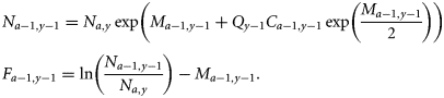
Process equations

The process equations for the baseline model can be expressed in a state space form as a Leslie matrix (Leslie, 1945, 1948), where the numbers N at age a + 1 in year y + 1 are derived from N at age a in year y. The transition function for a single cohort is

1

where Z_a,y(=F_a,y + M_a,y) is the total mortality at age a in year y and is the sum of fishing mortality F_a,y and natural mortality M_a,y. The oldest age (12) is a plus-group.

The model is structured in a similar manner to the ICES assessment model (ICES, 2008a) with two periods, an early part based on VPA, and a separable model part for the last 13 years, calculated using Equation (1) but for year y – 1 derived from year y. The use of two periods complicates the modelling, but there were changes in the fishery in the 1990s, with a transition from a fleet working purse-seines to one predominantly operating midwater trawls; this led to changes in selection-patterns-at-age during that period. The formulation of F_a,y and M_a,y is as follows. M is estimated in the model as independent of age and year; other formulations allowing age or time-trends or a fixed value of M = 0.15 (ICES, 2008a) were tested (see model variants below). For the separable period, F is defined as the sigmoidal function

2

where S₁ is the age at 50% selection, S₂ the age difference from 50 to 95% selection, and ln(19) a scaling factor resulting from the choice of 50 and 95 percentiles as controlling variables (see Haddon, 2001, for a slightly different formulation). The annually varying parameter values for the selection ogive are related using a random walk:

3

S₁₀, S₂₀, and σ_s are estimated in the model. Other formulations with F_a,y independent of F_a−1,y and σ_s fixed a priori were tested (see below).

For the VPA period, the catches (C_a,y) multiplied by a factor (Q_y) are assumed to be exact, and N and F are calculated following Pope's approximation (Pope, 1972):

4

In the baseline model, Q_y and M_a,y are assumed independent of age and year. Always M- and F-at-age are estimated simultaneously.

Observation equations

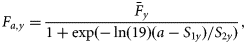
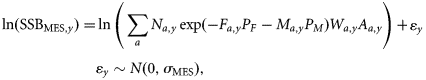
The observations are based on three sources of information: spawning-stock biomass (SSB) estimated from triennial mackerel egg surveys (MES), here referred to as SSB_MES, Z_Tag estimated from a tagging programme, and third reported catches. The first two are assumed to be unbiased. In contrast, reported catches are allowed to be biased by using an age-independent multiplicative factor Q_y [Equation (4)], which for the baseline model is independent of year. The observation equations are given below.

Estimates of SSB from triennial mackerel egg surveys

Estimates of SSB_MES are assumed to have a lognormal error distribution:

5

where P_F and P_M are the proportions of annual fishing and natural mortality occurring before the spawning season, W_a,y the mean weight, and A_a,y the fraction of adults all estimated without error (ICES 2008a).

To estimate the modelled SSB from the population N, the plus group is also required, although this is not fitted elsewhere in the objective function and does not follow from the N_11,y, but instead uses the formulation from Patterson and Melvin (1996) with F_11,y the fishing mortality at the oldest true age. The plus group N_12+,y is estimated directly from the plus-group catch Q_yC_12,y as

6

Estimates of total mortality from tagging studies

Using tag return data for fish belonging to year class y, the total mortality Z(i, j, y), between years i and j is obtained using the Jolly–Seber estimator (Ricker, 1975):

7

where R(i, y) is the number of tagged fish of year class y that were released in year i, R(j, y) the number of tagged fish of the same year class that were released in year j (j > i), and Σr(i, k, y) the numbers of such tagged fish that were recaptured in the years k summed over all k > j. The error in the estimates of Z is assumed to be normally distributed:

8

The standard deviation σ_T is estimated in the model.

Reported catches

The catch equation is modified to account for potential bias in reporting. The reported catches are modelled as a fraction (1/Q) of the true catches, and they follow a lognormal error distribution:

9

In the baseline case, σ_c,a is assumed to be independent of year and age and is estimated in the model. Model variants with age-dependence of the standard deviation σ_c,a (O'Brien et al., 2001; Simmonds et al., 2001) were also tested (see below).

Process and observation equations were set up using the Bayesian Markov Chain Monte Carlo (MCMC) framework WINBUGS (Spiegelhalter et al., 2003), which was used for both parameter estimation and diagnostics.

Data

Commercial catch data

For NEA mackerel, ICES assembles catch-at-age data annually. Data for ages 0–12+ covering the period 1975–2007 (ICES, 2008a) were used.

SSB from triennial mackerel egg surveys

ICES coordinates the triennial mackerel and horse mackerel egg survey (ICES, 2009c), and the data collected are used to estimate the total annual egg production (TAEP) by spawning mackerel along the 200-m depth contour west of the British Isles. Then, by making estimates of fecundity and atresia per gramme of female (ICES, 2005), the SSB of NEA mackerel can be calculated. These estimates of egg production are based on the abundance of eggs at development stage I, taking into account duration at that stage. Estimation, however, assumes that there is zero mortality of the eggs before capture during the relatively short stage I, which is clearly not the case. Here, we use specific values for egg mortality (Portilla et al., 2007) and directly consider the variation in duration at stage I attributable to temperature (Lockwood et al., 1981), giving a revised series of triennial estimates of SSB (SSB_MES). The surveys are carried out triennially because of their high cost and, because there are only six surveys from 1992 on, it is difficult to estimate precision σ_TMES within the Bayesian model, so the parametric bootstrap method reported by Simmonds et al. (2003) was used to provide values for σ_TMES.

Other methods have been proposed for estimating the spatial sampling precision of the egg survey. The ICES survey working group examined the variance for its more limited calculations in 2005, but with the additional factors included here, it is not complete. Imrie et al. (2003), for example, gave more precise estimates, with standard deviations of ∼80% of the estimates used here. To test the influence of precision on the results, different values were tested in the model (see later). The full procedure followed for calculating total egg production and its precision is not given explicitly elsewhere, so it is briefly included here as Appendix 1. As the method used to estimate precision involved several different types of distribution associated with different factors (egg abundance, fecundity, mortality, etc.), the parametric distributions used in the model to describe the error in the observations were obtained by fitting to the bootstrap distributions by year (Figure 1). The precision used in the baseline model depends on the year of the survey and is approximately equivalent to a CV of 30%.

Figure 1.

Estimated log(SSB) from bootstrap analysis of 6 years of triennial mackerel egg survey data (points), including errors in stage I egg abundance, egg mortality, fecundity, and atresia and fitted lognormal distributions (lines).

Total mortality from tag information

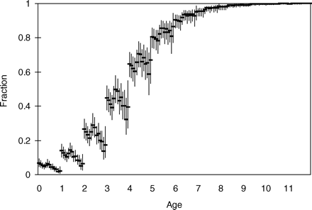
A tagging programme for NEA mackerel has been carried out in most years from 1983 on. A single missing year in the tagging programme, however, removes two estimates of annual mortality, and continuous data are available only from 1988 to 2003. Here, the tag-data estimates of Z are based on ratios between the number of tags recovered from consecutive releases (6). These estimates are only sensitive to the variation in initial tagging losses, not to the magnitude of the tagging losses, and, most importantly, they are independent of the proportion of catches sampled. The tag estimates of Z are highly variable (Figure 2a), with little consistent structure, over either time or age. The noise is so great that Z at some ages in some years is negative; this could be removed by smoothing, but doing so would distort the error structure, and for this analysis, it is important to bring the correct level of variability into the analysis. The variability may be caused by variation in initial tagging losses, the small numbers of tags recovered, and errors in age determination (Antsalo, 2006). The absence of time-trends in Z is not surprising, because the ICES assessment (ICES, 2008a) shows only a relatively small range of mean F_y. It might have been expected, however, that the estimated Z from tags would be age-dependent if we interpret the relative increase in abundance at ages 2 and 3 in the catches as increasing mortality with age. However, this signal is not seen in the data (Figure 2a). In the absence of any clear dependence of Z with age or time, the average Z over all years and ages was calculated, and the distribution of observations was fitted using maximum likelihood. A normal distribution described the variability of the observations around the mean (Figure 2b) and was used for the initial choice for the Bayesian prior, although the standard deviation (σ_T) is estimated in the model to allow for improved fit to the data by year or age. This choice is discussed further below.

Figure 2.

Estimated total mortality (Z_Tag,a,y) by age and year from tag data. (a) Point values and (b) a pdf with fitted Gaussian distribution (see text).

Model selection

Uninformative priors were used for all input parameters in the initial (baseline) model (Appendix 2). For the initial state vector, by age in the last year N_a,1, and by year N_11,y truncated (>0), normal distributions centred on the ICES stock assessment estimates (ICA method), and wide standard deviations (σ > 40 N) were chosen. Generally, the influence of priors was tested by increasing and decreasing the central value of a group of prior distributions by a factor of 10 (keeping the priors for all other parameters fixed), and ensuring that the influences on posteriors were negligible. Except M, the model was not sensitive to any of these priors, and the posterior distributions had well-established peaks and distributions much tighter than the priors, well away from any truncation. For M, a gamma prior was used because both truncated normal and uniform distributions lead to a small spike near zero in the posterior. Although the spike had negligible impact on mean or variance of the posterior, a gamma distribution, though more informative, is also biologically more plausible because it reduces the probability of an extremely low M. To test the influence of starting values on the results and to confirm convergence in parameter estimates, three MCMCs were initialized with different starting values for the estimated parameters (Appendix 2). Using Metropolis–Hastings selection criteria (Spiegelhalter et al., 2003; Figure 3a), the model initially converged in around 4000 iterations, so a burn-in period of 5000 iterations was discarded. Three parallel chains of two example parameters Q and M illustrate convergence (Figure 3b). Some 30 000 iterations gave convergence for F, M, and Q, but substantially shorter runs could give differing results for Q and M because the chains could be non-overlapping for several thousand iterations in a sequence (Figure 3b). The Gelman–Rubin criteria (Gelman and Rubin, 1992; Figure 3c) reveal convergence of the posterior distributions by ∼20 000 iterations after the burn-in period. Therefore, after a burn-in of 5000 iterations, the chains were run for an additional 30 000 iterations. For the calculation of the mean and distribution of parameter values, all 90 000 values, 30 000 from each of the three chains, were used without thinning (see King et al., 2009, p. 136, for a discussion of thinning). For Figure 3 (and, later, for Figure 6) and for the calculation of Bayesian p-values, only every 30th sample was retained, removing autocorrelated samples and still providing sufficient independent samples from the joint posterior distribution.

Figure 3.

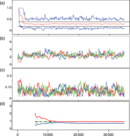
Example of fit criteria for the baseline model in WINBUGS. (a) Metropolis acceptance rate criteria showing convergence by ∼4000 iterations; data used are from 5001 to 35 000. Estimates of (b) Q and (c) M over iterations 1–35 000 for three chains thinned to 1/30. (d) Gelman Rubin statistic (for Q), which examines the variance within and across chains; the red line should be above 1 and asymptotic to it, the green and blue lines should be asymptotic to a final value; convergence occurs with 20 000 iterations.

The model results reveal strong negative correlation between Q and M. This implies moving removals from the population between linear and exponential processes. There was concern that this non-linear aspect might cause problems. This was checked first by examining the extent of the non-linearity; it amounts to a departure of ∼2% from linearity over the range of F and M values in the model. Nevertheless, to be sure that the effect was negligible, the baseline model was rerun with a simple transformation so that M was derived non-linearly from the prior such that both Q and M depended linearly on their priors. The model results were indistinguishable from those without the transformation.

Several model variants were also examined to evaluate the sensitivity of the results to model choices. The objective in exploring alternatives was both to select the best level of parametrization and to test the sensitivity of the conclusions to choices in parametrization. The different models were compared through two criteria. First was the deviance information criterion (DIC; Spiegelhalter et al., 2002), which is analogous to Akaike's information criterion in a maximum likelihood framework and is calculated from the samples of the three converged MCMCs. This method is provided within WINBUGS. Part of the calculation involves the computation of the effective number of parameters or model complexity, pD, accounting for between-parameter correlation; occasionally, the method used in WINBUGS can give negative values for this parameter. An alternative formulation based on deviance (Gelman et al., 2004, and used in Tremblay et al., 2006) has been proposed to make comparisons of DIC using a slightly different measure. However, negative values for pD suggest that some aspects of these models are less than ideal, so the results have been discarded. Second, Bayesian p-values (Gelman et al., 1995, 1996) were obtained from 1000 parameter sets sampled from the posterior distribution (taking every 90th sample in the three chains). These were loaded into R using the input routines from CODA (Best et al., 1997). Bayesian p-values are not analogous to the values of p in a standard significance test, but rather express how well the model fits the observations. The procedure (Gelman et al., 1996) is to take a sample from the joint posterior of parameter estimates (catch/Q and σ_c,a to compare with reported catches, Z and σ_T to compare with the mortality calculate from tag-return data, and SSB and σ_TMES to compare with SSB_MES). Then, for each parameter sample, the likelihood of the real observations is calculated and compared with the likelihood of a simulated set of observations drawn using the joint posterior distribution of parameters, including values of σ. Ideally, 50% of the simulated sets will have a greater likelihood and 50% a lesser likelihood than the observations used to fit the model; in this case, the p-value would be ∼50%, indicating a good correspondence in terms of both mean and distribution between model simulation and observations. The p-values for each dataset were calculated separately to evaluate the fit to each source of information separately. The log-likelihoods of the three observation components are summed to obtain to estimate the p-value for all datasets.

This procedure checks whether a model really captures the statistical properties (e.g. mean, variance, distribution) of the observations adequately. Using these two criteria (DIC and Bayesian p-values), we selected a single baseline model. The other models were then used to illustrate the sensitivity of the results to model assumptions. Conditioning was similar for all models, except where the length of the separable period is changed (options 5, 6, and 7 below), and the SBB_MES values were calculated differently (option 8 below). In all, 15 major variants were tested, listed below.

Model variants in catch-at-age constraints

To test the effect of the length of the period during which the fishing mortality is assumed separable, three more options were tested. Always, the preceding years were evaluated using a VPA based on starting ages for 1 January for the first year of the period used to fit a statistical catch-at-age model.

1. FS1, fixed selection with independence-at-age. Catch selection is based on 11 independent parameters at age scaled to independent annual values of F, with standard deviation (σ_c,a) assumed to be independent of age, to match the ICES Working Group settings (ICES, 2008a):

   

   10
2. FS2, fixed selection. Catch selection is based on a two-parameter logistic function, and standard deviation (σ_c,a) is assumed independent of age. It is scaled to independent annual values of F_y at the oldest ages:

   

   11
3. FSσ1, varying σ_c,a with age in Equation (9). F-selection is based on a two-parameter logistic function, but with σ_c,a following a parabolic function of age. A model with the three parameters required to define the parabolic function for σ_c,a was tested, but it would not converge so was discarded. A second version of σ_c,a with two of the three parameters for the parabola derived from studies of herring (Clupea harengus) market sampling (Simmonds et al., 2001) was used. This yielded a minimum σ_c,a at age 3.5, and curvature C = 0.006. The values of σ_c,a were scaled to fit by changing σ_min [Equation (12)]. In the classic parabolic equation (A + Bx + Cx²), the coefficients A and B affect both location and the magnitude of the minimum. Here, we use a formulation for σ_c,a based on two independent parameters, a_min and σ_min, the age and magnitude of σ_c,a at the minimum:

   

   12

   where ⁠, and B = 2 Ca_min. This formulation of the parabola converges faster and has a lower DIC.

4. SSP as baseline model, but with a smoother selection pattern. The variance parameter in the year-on-year change was constrained by setting σ_s to 0.5 × σ_s, the last parameter estimated in the baseline model run. This is a compromise between fixed and flexible selection by year.

• 5. SP15, extended separable period by 2 years, 1993–2007.

• 6. SP17, extended separable period by 4 years 1991–2007.

• 7. SP21, extended separable period by 8 years 1987–2007.

Model variants involving SSB_MES

The standard deviation σ_MES [Equation (5)] for SSB_MES is derived from the survey data and treated as model input. As the value depends on the calculation method (Appendix 1) and differs among years, the sensitivity of model results to the assumed value was evaluated. This led to three additional input options.

• 8. IEM, estimates of SSB_y derived using year-independent egg mortality.

• 9. var_TE × 3, standard deviation σ_TMES increased by a factor of √3.

• 10. var_TE/3, standard deviation σ_TMES decreased by a factor of √3.

Model variants with time- and age-dependence in M and Q

To test for the effect of potential time- and age-trends in catch and M, several options were tried.

• 11. WGM, fixed M equal to the ICES Working Group value of 0.15.

• 12. MTA, a linear trend in M-at-age starting at M₀ (M₀ > 0) for age 0, changing linearly to M from age a_b (a_b > 0) on:

  

  13
• 13. TMY, a linear time-trend in natural mortality, M_y, with the slope Q_ms with a lower limit of zero in all years. For convenience, the equation is referred to the midpoint in time, y_mid (1991). For years before 1983 where no tagging data are available, M_y was made equal to M₁₉₈₃, the last estimated year, to ensure the trend did not continue through years with no data on Z:

  

  14
• 14. TCY, a linear time-trend in catch multiplier, Q, with the slope Q_s having a lower limit of 1, meaning no underreporting:

  

  15
• 15. RWCY, a random walk in catch multiplier, Q, in time:

  

  16

Sensitivity to terminal year in the dataset

Since 2005, there have been changes in enforcement, potentially changing Q_y thereafter, so sensitivity to the last few years of data was checked. As SSB_MES values are available only once every 3 years, 3 years of data were removed, leading to option TD3, truncating the data, and the model by 3 years to the terminal year of 2004.

Results

Baseline model

Estimated values of F were similar to those estimated by ICES (2008a; Figure 4a), matching the early part of the time-series, but giving lower estimates in recent years. There was little difference between the mean and 2.5th and 97.5th percentiles of the posterior distributions using the full time-series 1975–2007 and the truncated series 1975–2004, indicating a lack of sensitivity to the recent data. However, as expected, Bayesian estimates of SSB differed substantially from the ICES estimates, with a general increase in line with the estimated additional unaccounted catch (Figure 4b). The modelled catch showed a clear increase in selectivity with age, with less variability between years than between ages (Figure 5). Always, except for option 11, WGM, F and M were estimated separately to ensure that uncertainty in M is included explicitly in the model. Unsurprisingly, the catch multiplier Q and the mortalities Z, F, and M were correlated, although the highest correlation was between Q and M (correlation coefficient −0.75). Correlation between Q and Z was less (correlation coefficient −0.46). The three MCMCs cover the same distribution of Q and M, and the joint posterior pdfs (probability density functions) are reasonably well-established (Figure 6), demonstrating that the model results are repeatable. The 95% intervals show that Q lies between 1.7 and 3.6 (Figure 6). The estimates of M lie between 0.017 and 0.20 (Figure 6), with the value M = 0.15 used by ICES situated in the upper part of the posterior distribution [p(M < 0.15|data) = 0.84]. The Bayesian p-values for SSB_MES (Table 2) were poor compared with those for catch and tag mortality data, partly because of the difficulty in describing a pdf with such a small number of observations (six). For example, separating catch observations into groups of six can give similarly large deviations on Bayesian p-values for the subsets. This suggests that small numbers of observations may not be well modelled, although the Bayesian p-value for the baseline model at 60% was close enough to 50% to indicate that overall the model fits the data reasonably well.

Table 2.

Model performance shown as Bayesian p-values by data type (values close to 50% are optimal, values above 95% or below 5% should be avoided), and DIC values giving the effective number of parameters compensating for correlation between parameters (pD).

			Bayesian p-values				DIC
Variant	Name	Description	SSBMES	Catch	Tags	Total	pD	DIC
0	BL	Baseline model	90.9	50.0	49.6	59.0	19.4	−35.3*
Model variants in catch-at-age constraints
1	FSI	Fixed independent selection at age	80.3	49.9	50.1	55.0	45.9	22.3*
2	FS2	Fixed two-parameter logistic selection function	80.6	49.2	50.4	54.9	39.9	19.4*
3	FSσ1	One-parameter parabolic variance function for catch-at-age	89.9	99.9	51.0	99.8	41.6	−29.8*
4	SSP	Baseline with smoothed selection pattern by year	88.9	49.9	50.4	58.1	30.0	−21.0
5	SP15	Sep Period +2 years = 15 years	89.7	49.9	49.8	58.2	30.4	−17.6
6	SP17	Sep Period +4 years = 17 years	92.7	50.4	50.4	59.6	48.1	44.4
7	SP21	Sep Period +8 years = 21 years	94.4	50.0	50.1	60.0	59.4	209.2
Model variants involving SSBMES
8	IEM	Constant (all years) mortality	93.0	50.0	49.7	60.4	15.1	−41.7
9	varTE × 3	SSBMES variance × 3	98.0	45.0	50.1	98.0	4.9	−43.6
10	varTE/3	SSBMES variance/3	97.3	49.8	49.8	60.9	23.3	−34.0
Model variants with time and age dependence in M and Q
12	TMY	Trend in M with year	88.2	50.0	50.1	58.3	16.0	−41.8*
13	TMY	Change in M at young age	87.9	50.2	49.2	57.3	37.7	−19.6*
14	TCY	Trend in Qc with year	88.6	50.2	49.8	58.6	21.2	−33.0*
15	RWCY	Random walk in Qc with year	86.9	49.5	49.7	56.5	3.9	−70.0

Only models marked with an asterisk are comparable.

Figure 4.

Median and 2.5 and 97.5 percentiles of population and exploitation estimates 1975–2007 (black) and 1975–2004 (red), compared with ICES assessment values (ICES, 2008a; blue) for (a) fishing mortality (F), and (b) SSB.

Figure 5.

Estimated selection pattern in the baseline model, expressed as a fraction of F-at-age (in age groups) for the years 1995–2007 (from left to right in each age group).

Figure 6.

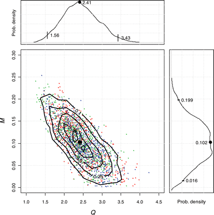
Joint posterior distribution from 1000 values (by thinning 1/30) from the three MCMCs showing estimates of natural mortality (M) vs. the catch multiplier (Q). Contours are at 0.10, 0.25, 0.50, 0.75, and 0.90. Intervals on posterior distributions of Q and M are 0.025, 0.50, and 0.975. The plot shows that the three chains fully overlap and that there is negative correlation (correlation coefficient = −0.75), apportioning removals between catch and natural mortality. Although Q and M are compounded, the distribution of Q does not include unity. See text for a discussion of the scaling of Q and M.

Model variants

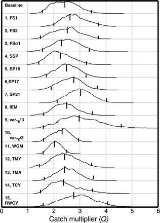
The performance of some of the different model variants can be compared through differences in DIC and Bayesian p-values (Table 2). Not all the models are directly comparable, because some use data subsets. Although the model results indicate that the baseline model performs best overall, the choice is not entirely straightforward, because DIC and Bayesian p-values occasionally conflict. The results for the different variants were examined in terms of the pdf of Q (Figure 7). There is considerable similarity in the pdf from different variants (options), with none including Q = 1 in the 95% intervals (Figure 7).

Figure 7.

Posterior distributions, median, and 2.5 and 97.5 percentiles of the catch multiplier Q for different model variants by model number and acronym (see text).

Catch-at-age model variants

The models with catch-at-age selection constant over time (FS1 and FS2) had higher values of DIC than the baseline model with the more flexible separable period, but a slightly better p-value (closer to 50%) for SSB_MES data and similar p-values for the other two data sources (Table 2). FS1, the function with independent selection at age, followed the same general form as FS2, the two-parameter logistic function (Figure 8). For FS1, the variability at older ages suggested no differences in selectivity at age 7 and older. FS2 gave the lower value of DIC, supporting the use of the logistic function. A parabolic function of σ_c,a age was used in model variant 3, i.e. FSσ1. Only one of the three parameters of the parabolic function for σ_c,a was estimable. When all three parameters of the parabola were fitted, the posterior of the catch multiplier Q was equal to its prior (uniform from 0.1 to 30), indicating overparameterization. FSσ1 gave a slightly higher value of DIC and a very poor p-value for catch (Table 2), suggesting that the fit was good for some ages but not for all, posing a question as to the suitability of the parabolic function. For this reason, the parabolic variance models were not evaluated further.

Figure 8.

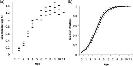
Model variants FS1 and FS2, median, and 2.5 and 97.5 percentiles of fitted selectivity functions, constant over year from 1992 to 2004: (a) FS1 independently at age, with nine parameters referred to age 5; (b) FS2 as a two-parameter logistic function.

Sensitivity to changes in the period used for the separable model was tested by changing the number of years from 13 to 21 (Models SP15, 17, and 21). The data inside the separable period were treated differently from the data in the VPA period, leading to a different dataset being used in the objective function, so comparison of the DIC among these variants is not appropriate. However, the changes did not influence estimates of Q except when the 13-year period (baseline model) was extended to 21 years (Model SP21), but even there, the changes in Q were relatively small (Figure 7). Shortening the separable period, i.e. extending the VPA section, was tested, but it resulted in a negative pD, so this option was discarded.

Model variants involving SSB_MES

Although annual estimates of egg mortality were significantly different (Portilla et al., 2007), stage I mortality was not investigated explicitly. To test whether the assumption of independence by year was influencing the results, Model 8 with fixed egg mortality across years (FM) was tested, and it showed no important differences from the baseline model for any model output parameters.

As the precision of the SSB_MES is input to the model, its influence is explored in Models 9 and 10, var_TE × 3 and var_TE/3. The variance of SSB_MES is the result of the variance of several factors (Appendix 1). The precision in each factor was obtained from analyses of the western egg survey (which constitutes ∼85% of the total egg abundance), and scaled to the full survey (assuming a constant CV). The variance of the different factors was assumed to be independent. Although this is likely to be true for measurements of atresia, fecundity, and egg abundance, errors in egg mortality may be correlated with egg abundance. The effect of ignoring such a correlation would be to overestimate the variance in SSB_MES.

Increasing or decreasing the assumed variance for SSB_MES (Models 9 and 10) substantially reduced the utility of the fit as judged through a Bayesian p-value for SSB_MES, from 91 to 98 or 97%, respectively. It was possible to obtain a slightly improved Bayesian p-value relative to the baseline model value by manipulating the standard deviation to 0.95 × the value used in the analysis, suggesting that a slightly lower standard deviation may be appropriate. An overall factor of three changes in variance is well outside the range that could be expected, but it resulted only in small changes to estimates of the catch multiplier Q (Figure 7). Greater changes in var_TE were tested, but a model with var_TE × 4 gave negative values of pD, so models with higher factors were discarded.

Model variants with time- and age-dependence in M and Q

The model formulations discussed above assume that natural mortality M and catch factors Q are constant with year. Further options tested were: Model 11, WGM, M fixed equal to the ICES Working Group value of 0.15; Model 12, MTA, a linear trend of M_a at young age; Models 13, MTY, and 14, TCY, a linear trend of M_y or Q_y in time, and Model 15, RWCY, a random walk for Q_y in time. Fixing M (at the Working Group value) is artificial because the value is not established precisely and, as expected, results in tighter intervals in the posterior of Q (Figure 7). The posterior distribution for Q lay entirely within the posterior distribution estimated using the baseline model. For neither M_y nor Q_y could significant trends in time be estimated (Figure 9b and c), but in the posterior, the probability of M_a > 0.15 increased at young ages (<5) and decreased at older ages (Figure 9a). The posterior probability of Q_y increasing with time (slope = 0.06 per year; Figure 9b) is ∼0.8. In contrast, there is effectively no real evidence of an increasing M_y with time because the posterior for M_y is without any meaningful trend with time (slope = 0.003 per year; Figure 9c).

Figure 9.

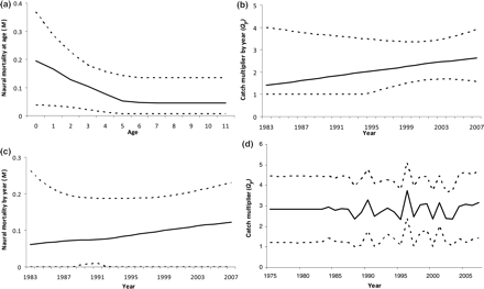
Median and 2.5 and 97.5 percentiles of posterior distributions for (a) natural mortality (M_a) changing linearly with age at young ages, model MTA; (b) catch multiplier (Q_y) changing linearly with time, model TCY; (c) natural mortality (M_y) changing linearly with time, model MTY; (d) random walk in Q_y with time, model RWCY.

In the cases where there were some signs of trend in the predictions (linear Q_y and M_a), the DIC increased, suggesting that the model had less explanatory power. For the case of a linear M_y, the DIC decreased, but there is potential for some formulations with a trend in M_y to give negative values of pD, indicating that the models are questionable (see above). Always where this happened, the model formulations were discarded, so the specific example given here (Figure 7) should be regarded with some caution.

Our main conclusion is that always, the changes in the posterior distribution of Q with model choices were small, the greatest effect being for the trend in Q over time, reducing the value for the early part of the time-series. This option suggests a lower mean value overall, but this comes from a reduction in Q_y before 1990; the mean for Q_y from 1992 to 2007 (the period over which the egg survey data are available) is similar. In this case, the positive slope in time yielded higher values of Q_y in the recent past (Figure 9b). The addition of a random walk with time to Q_y fitted much better to the tag-mortality data. Again, however, it was not possible to detect a significant year-on-year change (Figure 9d). Nevertheless, it seems unlikely that there is no variability over time, but rather that the data we have were too noisy to estimate variability or that such a model was overparameterized. The resulting annual factors (Figure 9d) show consistency from 1975 to around 1988, because there is no egg survey or tag-mortality data to which to fit. From 1989 the variability increased, explaining some of the variable mortality in tag data and annual variability in catch-at-age as unaccounted mortality. The low DIC (Table 2) indicates that this model might have increased explanatory power, but the value of pD is unusually low and some formulations give a negative pD, opening to question the validity of this option of the model.

Z derived from tagging data

The only aspect of the model that was not varied directly in model exploration was the use of the estimates of Z derived from tagging data, but as discussed above, the fit to these data does depend on some of the other options explored. With the assumptions of constant or linearly changing coefficients on catch, the relationship between observed and modelled estimates of total mortality was poor. The modelling results suggest that there was very little signal in the total mortality for ages 2–10 from 1983 to 2005. One reason for this is that F_bar for that period has a mean of 0.29 (s.d. = 0.06). Most of the signal in Z_a,y is attributable to age, although this depends to some extent on assumptions about M_a in the model. As discussed above, the tag data are very noisy and even include negative estimates; for the baseline model, the variance in the tag-based estimates of total mortality exceeds the variance of the modelled values by >6 times, which perhaps explains why a poor fit resulted. The distribution of errors and the Bayesian p-value of 50% strongly support the use of a Gaussian distribution to describe the error (Figure 2). Given the poor fit and the relatively well-supported choice of a Gaussian distribution, there was little scope for further exploration. However, as discussed above, if Q_y is allowed to vary from year to year, through the addition of a random walk component, and M is allowed to increase at young ages, the fit to the tagging data improves, but only slightly.

Discussion

The Bayesian approach with multiple models adds to the confidence in the analysis and provides well-supported conclusions. The NEA mackerel stock may be much larger than previously thought. For the NEA mackerel evaluation overall, the model results were driven by estimates of SSB, from egg surveys for the period 1992–2007, and mean estimates of Z from tag data for the years 1988–2003. This analysis leads to estimates of SSB that are significantly greater than the ICES estimates (Figure 4), and this possibility is recognized in the ICES Advice (ICES, 2008b). The increased SSB estimate is provided by increasing catch using a catch multiplier while maintaining estimates of F similar to the ICES estimates, because both catches and numbers are similarly scaled.

The posterior probability mass functions of Q were always high for values >1, compatible with reported catches being significant underestimates of removals by fishing. The lack of sensitivity of the posterior estimates of Q to model choices (Figure 7) suggests considerable robustness for this conclusion. In October 2005, Scottish fisheries regulation enforcement officers obtained information from fisheries processors and found discrepancies between the official declared landings and the tonnages reported as processed by the factories. These figures were subsequently reported to ICES and corresponded to around 1.6 × the quota for the Scottish pelagic fleet (ICES, 2006), although this factor assumed that landings by those fleets were accurately reported when landed elsewhere. The same information indicated some underdeclaration of landings by Irish vessels into Scotland, although those constitute only a small part of the total landings for that fleet (ICES, 2006). In 2003, Remøy et al. (2003) analysed Irish export figures and estimated an overquota summed over the period 1988–2002 of 677 000 t, which would have constituted about 1.7 × the quota concerned. However, these were quite controversial claims, and there was some dispute over the validity of the study (Marine Times, 2003).

In addition to landed catches, other potential sources of removals which were not included in the assessment were the discards from most of the mackerel fishing fleets. Up to 2005 when the inspections improved in both the UK and Ireland, discarding from these refrigerated seawater (RSW) fleets had been observed to be a very small proportion of the recorded landings (ICES, 2006). In contrast, the freezer trawler (FT) fleet, which has a small proportion of the quota, was observed to discard at higher rates; Borges et al. (2008) reported annual levels of discarding of mackerel of ∼12 000 t by the Dutch FT fleet over recent years (2002–2005). This represented an additional 42% over their landed catches (ICES, 2008a), but these discard tonnages are not included in the catch estimates of ICES, because their age composition has not been estimated. However, in total, these known unaccounted FT fleet discards corresponded to a small (<5%) proportion of the total ICES catches. In some fisheries, slipping (discarding without bringing on board) does take place; there are two major reasons for this. First, mixed catches particularly of mackerel and herring can be slipped because the market prices for mixtures of species are lower; second, excess catch in the purse-seine or trawl fleets can be slipped once RSW tanks are full. Obtaining better data on discards, at the youngest ages, and including such information in the model, might potentially give a shallower selection ogive if, as is likely, larger proportions of younger fish are discarded. This might fit better to the tagging data, but would probably make little difference to the estimated abundance of the older mackerel that contribute most to the fishery and the SSB.

Huse et al. (2008) studied survival from purse-seines and showed that up to 80% of mackerel concentrated in the purse can die on release. The extent of such practice is difficult to estimate, because the tonnages are not properly recorded, and in some cases may be hidden because they are illegal. Overall, the posterior median Q of 2.6 may appear to be a bit high. However, combining the Scottish factor of 1.7 with discard rates of 1.4 in the Dutch FT fleet (Borges et al., 2008), along with additional unknown mortality caused by slipping surplus or mixed catches in almost all fleets, and allowing for some mortality of escaping mackerel, it is quite easy to get close to a value of Q of 2.6. Certainly, values above the 2.5% level of 1.7 are plausible.

Natural mortality, M, was not significantly different from the constant value assumed by the ICES Working Group (ICES, 2008a). There was also weak evidence coming from the tagging data for a higher M at young ages. However, there was no indication of a time-trend in M. In this context, it is important to remember that the distinction between F and M is that fishing is associated with a rising mortality rate at age and natural mortality is associated with a flat or falling mortality rate at age. If elements of M were to rise with age, the model will have assigned these as increased catches.

The lack of sensitivity of the estimated Q to the variance of SSB_MES suggests that its value is not critical, and even if not entirely accurate, the exact magnitude of the errors may not be important in this context. The value explicitly includes all the uncertainty in egg abundance of which we know (including uncertainty in egg mortality). The baseline model used year-dependent egg mortality, which is supported by analysis of the data, but using a year-independent estimate (McGarvey and Kinloch, 2001) did not alter the conclusions. Only bias in the estimates caused, for example, by the assumption of constant mortality across egg stages could influence the results further. It is important to note that, in the baseline model, the mean of the estimated median biomass from all egg-survey years is slightly higher than the mean from SSB_MES observations, suggesting that there are other signals in the data giving even larger biomasses. This certainly does not suggest that the corrections for fecundity, atresia, and egg mortality are too great, nor that substantial numbers of non-mackerel eggs are misidentified as mackerel.

Given the poor fit of the model to the tag-mortality data, its overall utility may be questioned. As stated above, the variance is high; for instance, the observation variance is six times the variance in the signal, leading in some cases to negative estimates of mortality estimates. These negative values are just an expression of the noise in the data resulting from highly variable numbers of tag returns. Nevertheless, the Bayesian p-values for tag mortality of 49.6% suggest that the information in the mortality data is explained appropriately within the model. As the method used for estimating tag mortality uses the ratio of two sets of returned tags by cohort [Equation (7)], a systematic error in tag-estimated Z over all years seems unlikely. The high level of noise in the tagging data is unsurprising in such a large fish population, for which it is difficult to tag sufficient individuals. Therefore, the model results rely almost exclusively on the mean of all tag mortalities, treating the detail in the data by age and year as noise.

There may be other sources of error in biomass, such as a mismatch between the fished and the surveyed stock, although this is likely to be small given that the East Atlantic is treated as containing one large stock of mackerel, so the potential for stock identity issues is small.

Conclusions

The Bayesian approach with multiple models adds confidence to the results. The baseline model estimates that the NEA mackerel stock is larger than previously thought. Higher biomass from the mackerel egg survey was explained by inflating the removals of mature mackerel by the fishery. None of the models estimate a 95% range of catch multiplier from 1992 to 2007 that includes unity (no additional catch). All the alternative model options led to similar, or usually slightly higher, levels of fishery removals. Therefore, in our opinion, the conclusions are robust to changes in model structure, estimated variance in the egg survey, trends in natural mortality, M, at age or over time, and trends in unaccounted mortality over time.

Acknowledgements

We thank the two referees and the editor who spent considerable time and provided an attention to detail that we believe improved the paper considerably. We also thank all those who over many years assembled the catch, tag, and survey data, without whom none of the analysis would be possible. We received modelling advice from a number of sources, but specifically acknowledge Ruth King for her help with the Bayesian modelling in general and Steve Smith for advice on calculating Bayesian model complexity.

Appendix 1

Calculation of mackerel SSB from the ICES triennial mackerel and horse mackerel egg surveys (TMHMES)

ICES coordinates the triennial mackerel and horse mackerel egg survey, TMHMES (ICES, 2005), reports estimates of total annual egg production (TAEP) of the stock (ICES, 2005), and derives an estimate of SSB. The method and results for precision calculations to 2003 are given in Simmonds et al. (2003). The same method was applied to the 2004 and 2007 surveys. Historically, the ICES results have been presented without the inclusion of annually estimated egg mortality, i.e. assumed zero (McGarvey and Kinloch, 2001), so in recent years the survey has been fitted as an index of abundance, not as an absolute estimate. Here, the mortality was included because the information on absolute abundance is critical to the analysis, leading to a correction factor: SSB_MES,y = F_y SSB_{ICES–TAEP,y}, where the values of the correction factor F_y are calculated accounting for the estimated instantaneous mortality M_y and duration D_y1, over egg stage I:

where rln(D_y1) indicates draws from lognormal distributions describing the abundance weighted distribution of durations, and runif() a draw from a uniform random distribution describing the time points samples could be taken assuming sampling occurs at any time during stage I. This approach accounts for the sampling bias described in Dickey-Collas et al. (2003). All mortality estimates and their precisions are derived from samples collected in the western part of survey area, which holds typically 85% of the total NEA mackerel population. The factors for the whole area are expected to be similar. The values for the parameter M_y and the distribution of durations (D_y1, σ_y1) are obtained as described below.

Egg mortality M_y

The information on egg mortality was drawn from Portilla et al. (2007), which provides annual estimates of mean daily instantaneous mortality (M_y) across all egg development stages, using data from the surveys in western waters from Biscay to the west of Scotland, along with standard errors (Table A1). Although differences in mortality were observed among the development stages, these were not significant, so a mean mortality over all stages was used to apply to stage I. Annual daily rates of mortality were significantly different by year (Table A1), suggesting that annual values are preferable to a mean value across years. The values of M_y in Table A1 were used in the analysis, and their variance was added to the variance from Simmonds et al. (2003).

Duration of stage I (D_y1)

The duration D_y1 and its distribution are estimated from experimental studies reported in Lockwood et al. (1981); these values are used to derive a distribution of median duration at stage I weighted by egg abundance from 1998 to 2007 (Figure A1). A maximum-likelihood-fitted lognormal distribution, with σ = 0.189, which best explains the time for transition, is also shown. The mean value of D_y1 by year is given in Table A1. An additional stochastic element was estimated from the spread of hatch times also reported in Lockwood et al. (1981). A Gaussian distribution with variability proportional to duration has been fitted to the spread of hatch dates reported, yielding a CV of 0.049. Using a constant CV, implying variability proportional to duration, gives estimates of the stochastic variability of stage I duration. Combining the stochastic part with the temperature-based deterministic distribution of durations results in a slightly wider lognormal distribution, with σ increasing from 0.189 to 0.202 (Figure A1).

Figure A1.

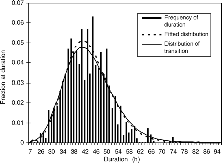
Fitted lognormal distribution of the duration at stage I derived from observed egg abundance and temperature by station from 1998 to 2007. The modified distribution incorporates a stage-transition variability used to estimate the distribution of durations and subsequently mortality at egg stage I.

For 2004 and 2007, where no separate annual estimate of egg mortality was available, the mean correction factor F_e of 1.44 was used. The resulting precision of the egg surveys of close to 30% includes estimates of errors in estimating egg abundance, egg mortality, atresia, and fecundity. The distributions derived from bootstrapping, and the fitted lognormal distributions used in the main model, are given in Figure 1.

Table A1.

Annual mean daily stage I and II egg mortality and stage duration (h; Portilla et al., 2007) and resulting correction factors and mackerel egg survey estimates of SSB (SSB_MES,y) including atresia, fecundity, and egg mortality.

Year	Daily mortality My	s.d.	Mean stage I duration Dy1	Correction factor Fy	s.d.	ICES TMHMES mackerel estimates	SSBMES,y including egg mortality
1992	0.665	0.021	43.3	1.71	0.015	3 370 000	5 760 000
1995	0.518	0.018	43.6	1.54	0.013	2 840 000	4 370 000
1998	0.623	0.025	42.6	1.64	0.018	3 750 000	6 150 000
2001	0.434	0.021	42.5	1.43	0.015	2 900 000	4 150 000
Mean	0.56		43.0	1.53
2004	0.56		43.0	1.53	0.015	2 750 000	4 210 000
2007	0.56		43.0	1.53	0.015	3 260 000	4 990 000

Appendix 2

Table of prior distributions and their parameters, and the three sets of starting values for the MCMC used for the baseline model.

	Priors		Initial conditions for the main model
Distribution	Parameters	Chain 1	Chain 2	Chain 3
N oldest true age (11)
T Y-1	Normal(µ, σ) > 10.0	8.0E + 4, 4.0E + 6	6.74E + 04	1.0E + 04	1.0E + 05
T Y-2	Normal(µ, σ) > 10.0	8.0E + 4, 4.0E + 6	6.11E + 04	1.0E + 04	1.0E + 05
T Y-3	Normal(µ, σ) > 10.0	8.0E + 4, 4.0E + 6	5.69E + 04	1.0E + 04	1.0E + 05
T Y-4	Normal(µ, σ) > 10.0	8.0E + 4, 4.0E + 6	7.27E + 04	1.0E + 04	1.0E + 05
T Y-5	Normal(µ, σ) > 10.0	8.0E + 4, 4.0E + 6	6.08E + 04	1.0E + 04	1.0E + 05
T Y-6	Normal(µ, σ) > 10.0	8.0E + 4, 4.0E + 6	8.07E + 04	1.0E + 04	1.0E + 05
T Y-7	Normal(µ, σ) > 10.0	8.0E + 4, 4.0E + 6	6.61E + 04	1.0E + 04	1.0E + 05
T Y-8	Normal(µ, σ) > 10.0	8.0E + 4, 4.0E + 6	7.11E + 04	1.0E + 04	1.0E + 05
T Y-9	Normal(µ, σ) > 10.0	8.0E + 4, 4.0E + 6	1.19E + 05	1.0E + 04	1.0E + 05
T Y-10	Normal(µ, σ) > 10.0	8.0E + 4, 4.0E + 6	7.09E + 04	1.0E + 04	1.0E + 05
T Y-11	Normal(µ, σ) > 10.0	8.0E + 4, 4.0E + 6	9.59E + 04	1.0E + 04	1.0E + 05
T Y-12	Normal(µ, σ) > 10.0	8.0E + 4, 4.0E + 6	1.72E + 05	1.0E + 04	1.0E + 05
N terminal year
Age 11	Normal(µ, σ) > 10.0	71 320, 5.6E + 6	7.38E + 04	1.0E + 04	1.0E + 05
Age 10	Normal(µ, σ) > 10.0	113 035, 8.9E + 6	1.02E + 05	2.0E + 04	2.0E + 05
Age 9	Normal(µ, σ) > 10.0	179 148, 1.4E + 7	1.60E + 05	4.0E + 04	4.0E + 05
Age 8	Normal(µ, σ) > 10.0	283 931, 2.2E + 7	2.72E + 05	8.0E + 04	8.0E + 05
Age 7	Normal(µ, σ) > 10.0	450 000, 3.6E + 7	3.47E + 05	2.0E + 05	2.0E + 06
Age 6	Normal(µ, σ) > 10.0	713 202, 5.6E + 7	5.12E + 05	4.0E + 05	4.0E + 06
Age 5	Normal(µ, σ) > 10.0	1 130 349, 8.9E + 7	9.27E + 05	8.0E + 05	8.0E + 06
Age 4	Normal(µ, σ) > 10.0	1 791 482, 1.4E + 8	5.18E + 05	1.0E + 06	1.0E + 07
Age 3	Normal(µ, σ) > 10.0	2 839 308, 2.2E + 8	3.25E + 06	2.0E + 06	2.0E + 07
Age 2	Normal(µ, σ) > 10.0	4 500 000, 3.6E + 8	4.99E + 06	4.0E + 06	4.0E + 07
Age 1	Normal(µ, σ) > 10.0	7 132 019, 5.6E + 8	7.60E + 05	4.0E + 06	4.0E + 07
Age 0	Normal(µ, σ) > 10.0	11 303 489, 8.9E + 8	5.47E + 05	4.0E + 06	4.0E + 07
Fbar
Fbar terminal year	Uniform(a, b)	0.001, 2	0.269189101	0.1	1.0
T Y-1	Uniform(a, b)	0.001, 2	0.30602243	0.1	1.0
T Y-2	Uniform(a, b)	0.001, 2	0.350189295	0.1	1.0
T Y-3	Uniform(a, b)	0.001, 2	0.310492461	0.1	1.0
T Y-4	Uniform(a, b)	0.001, 2	0.275209562	0.1	1.0
T Y-5	Uniform(a, b)	0.001, 2	0.249905656	0.1	1.0
T Y-6	Uniform(a, b)	0.001, 2	0.260652782	0.1	1.0
T Y-7	Uniform(a, b)	0.001, 2	0.232327736	0.1	1.0
T Y-8	Uniform(a, b)	0.001, 2	0.239031653	0.1	1.0
T Y-9	Uniform(a, b)	0.001, 2	0.308624558	0.1	1.0
T Y-10	Uniform(a, b)	0.001, 2	0.311775171	0.1	1.0
T Y-11	Uniform(a, b)	0.001, 2	0.304181787	0.1	1.0
T Y-12	Uniform(a, b)	0.001, 2	0.243885393	0.1	1.0
Age at 50% selection	Uniform(a, b)	0.1, 6.0	2.0	0.3	5.00
Age at 95% selection–Age at 50% selection	Uniform(a, b)	0.2, 6.0	2.0	0.3	5.00
Natural mortality M	Gamma(r, µ) × 0.15	1.5, 0.05	0.15	0.1	0.25
Catch factor Q	Uniform(a, b)	0.1, 30.0	1.5	30.0	0.15
Tau M (σ = 1/Tau0.5)	Gamma(r, µ)	0.001, 0.001	1.0	10.0	0.1
Tau s (σ = 1/Tau0.5), Age at 50% selection	Gamma(r, µ)	0.001, 0.001	1.0	0.1	0.05
Tau s (σ = 1/Tau0.5), Age at 95% selection–Age at 50% selection	Gamma(r, µ) > 0.05	0.001, 0.001	1.0	0.1	0.05
Tau c (σ = 1/Tau0.5), Random walk on age at 50% selection	Gamma(r, µ)	0.001, 0.001	1.0	10.0	0.1