-
PDF
- Split View
-
Views
-
Cite
Cite
Rüdiger Voss, Hans-Harald Hinrichsen, Martin F. Quaas, Jörn O. Schmidt, Olli Tahvonen, Temperature change and Baltic sprat: from observations to ecological–economic modelling, ICES Journal of Marine Science, Volume 68, Issue 6, July 2011, Pages 1244–1256, https://doi.org/10.1093/icesjms/fsr063
Close - Share Icon Share
Abstract
Temperature effects on Baltic sprat are many and include both direct and indirect effects. Increasing temperature is thought to increase the survival of all early life stages, resulting in increased recruitment success. We quantified the spatially resolved temperature trend for major spawning grounds and depth layers being most relevant for sprat eggs and larvae, using a three-dimensional hydrodynamic model for 1979–2005. Results confirmed an underlying positive temperature trend. Next, we tested these time-series as new explanatory variables in an existing temperature-dependent recruitment function and applied these recruitment predictions in an age-structured ecological–economic optimization model, maximizing for profit. Economic optimal solutions depended upon variability in temperature trajectories. Under climate-change scenarios, mean optimal fishing mortality and related yields and profits increased. The extent of the increase was limited by the general shape of the stock–recruitment model and the assumption of density-dependence. This highlights the need to formulate better environmentally sensitive stock recruitment models. Under the current knowledge of Baltic sprat recruitment, the tested climate-change scenarios would result in a change in management targets. However, to serve as a quantitative management advice tool, models will have to address the above-mentioned concerns.Voss, R., Hinrichsen, H-H., Quaas, M. F., Schmidt, J. O., and Tahvonen, O. 2011. Temperature change and Baltic sprat: from observations to ecological–economic modelling. – ICES Journal of Marine Science, 68: 1244–1256.
Introduction
There has been a general global warming trend throughout the past decades and for the European region, it has been calculated to be in the range of 0.4°C per decade (IPCC, 2007). Effects of climate-change-related temperature increase on marine ecosystems have been documented in many places, e.g. in the North Atlantic Ocean (Beaugrand, 2009) as well as in coral reefs (Hoegh-Guldberg et al., 2007). Such changes are affecting ecosystems on all trophic levels, i.e. from phytoplankton to carnivorous fish stocks (Beaugrand, 2009). In commercially exploited fish stocks, distribution patterns might change (Beaugrand, 2009) or stock dynamics could be influenced if stock–recruitment relationships turn out to be temperature-dependent (Lillegaard et al., 2005; Duplisea and Robert, 2008). Such changes in stock dynamics would inevitably have socio-economic impacts, because the fishing industry will be affected (e.g. fleet profitability: Bastardie et al., 2010; net economic production: Arnason, 2007). This requires adaptive management strategies to guarantee sustainability (Binder et al., 2010).
Management strategy evaluation (MSE) is a powerful tool for investigating and comparing different management options (Schnute et al., 2007). A number of frameworks have been established (e.g. TEMAS, Ulrich et al., 2007; FLR, Kell et al., 2007) and applied to a wide range of stocks (Dunstan and Bax, 2008; Dorner et al., 2009). Management goals are typically predefined and biologically driven (stock status) with subsequent (or parallel) economic considerations. MSE studies, including economics as well as climate-change effects, are, however, very scarce (Link and Tol, 2009). Nonetheless, conceiving strategies for more sustainable fisheries also requires an economic approach, for two complementary reasons. First, economic incentives determine how resources are used in a market economy. Second, unlike ecology, economics provide sound methods for operationalizing normative societal objectives, such as welfare and sustainability. Therefore, advice-giving organizations (in particular ICES) have recently broadened their scope to also exploring the potential of coupling ecological and economic considerations for integrated advice (ICES, 2009a).
In this study, we use Baltic sprat as an example of a feasible way to apply economic normative objectives (in this case, maximizing the net present value of resource rents) in an ecological–economic model of a fishery harvesting an age-structured fish population. We illustrate how dynamic economically optimal management trajectories of fishing mortality, yield, and stock size can be derived even when taking into account the effects of climate change. The results of this study are intended to provide an economic baseline scenario. Biological constraints have not been taken into account. This could be done by setting appropriate side conditions in the optimization, but for Baltic sprat, there is still a continuing discussion about the appropriate constraints. We used an age-structured ecological–economic model, because such models might result in significantly different management recommendations from classical biomass approaches (Tahvonen, 2008, 2009, 2010). Furthermore, using an age-structured approach fosters communication and data exchange between economists and stock assessment scientists.
In the Baltic Sea, sprat (Sprattus sprattus) is an ecologically important pelagic fish species (Kornilovs et al., 2001) as both a prey for top predators (e.g. cod and harbour porpoise) and a predator of zooplankton and fish eggs (Bagge et al., 1994; Köster and Möllmann, 2000a, b). Currently, it also represents the most abundant, commercially exploited species in the Baltic (ICES, 2010a). The Baltic sprat stock has displayed large fluctuations that were influenced by variable recruitment strength (Köster et al., 2003). Temperature appears to be one of the main drivers for recruitment success during all early life stages of sprat (Baumann et al., 2006a; their Figure 5). Higher temperatures result in: (i) lower egg mortality (Hinrichsen et al., 2007), (ii) faster egg development, resulting in lower predation mortality (Nissling, 2004; Petereit et al., 2008), (iii) higher larval growth rates, being coupled with better survival (Baumann et al., 2006b), (iv) higher larval prey abundance, i.e. Acartia sp. abundance (Möllmann et al., 2003; Dickmann et al., 2006), and (v) better juvenile growth and survival (Peck and Daewel, 2007).
Therefore, environmentally sensitive stock–recruitment models have been formulated that include temperature as an explanatory variable (ICES, 2010b). The model explaining most recruitment variability includes spawning-stock biomass (SSB), a larval transport index (bottom depth anomaly; Baumann et al., 2006a), and satellite data of sea surface temperature in May, recorded on a 2 × 2° grid (ICES, 2010b). However, sea surface temperature as recorded by satellite data might only be a rough indicator of temperatures experienced by sprat early-life-history stages. Eggs are usually found in 50–60 m depth (ICES, 2010c) and larvae, as well as juveniles, do not only inhabit a thin surface layer, but the upper 10 m of the water column (Voss et al., 2007).
The first objective of this study was therefore to confirm and quantify historical (1979–2005) temperature increase in the Baltic Sea in depth layers inhabited by sprat eggs and larvae/juveniles. Based on a spatially resolving hydrodynamic model for the Baltic Sea, we established a temperature time-series providing a full coverage of the potential distributional area of eggs and larvae/juveniles. The second objective was testing these time-series data as explanatory variables in the recruitment function to determine whether these data offered a better alternative to satellite data.
The third objective was to calculate optimal fishing mortality rates and corresponding stock size for a matrix of economic variables (costs and interest rate), as well as for environmental forcing variables (temperature and bottom depth anomaly). In a final step, we calculated optimal fishing mortalities, maximizing the net present value of resource rents under two climate-change scenarios. These final calculations should, however, be seen as only an illustrative example rather than real management advice, because some strong assumptions about species interactions and economic costs had to be made.
Material and methods
Temperature trends
To obtain vertically and spatially resolved temperature fields, a hydrodynamic model for the Baltic Sea (Lehmann, 1995) was utilized for 1979–2005. The hydrodynamic model is based on the free surface Bryan–Cox–Semtner model (Killworth et al., 1991), which is a special version of the Cox numerical ocean general circulation model (Bryan, 1969). A detailed description of the equations and modifications necessary to adapt the model to the Baltic Sea can be found in Lehmann and Hinrichsen (2000). A detailed analysis of the Baltic Sea circulation was done by Lehmann et al. (2002).
The model has a 5 km grid horizontal resolution and 60 depth levels. The thickness of the different levels is chosen to account best for the different sill depths in the Baltic. The Baltic Sea model is driven by atmospheric data provided by the Swedish Meteorological and Hydrological Institute (SMHI: Norrköping, Sweden) and river run-off taken from a mean run-off database (Bergström and Carlsson, 1994). The meteorological database covers the entire Baltic Sea drainage basin with a grid of 1 × 1° squares. Meteorological parameters, such as geostrophic wind, 2 m air temperature, 2 m relative humidity, surface pressure, cloudiness, and precipitation are stored with a temporal increment of 3 h. Prognostic variables of the model are the baroclinic current field, the three-dimensional temperature and salinity distributions, the two-dimensional surface elevations, and the barotropic transport. Physical properties simulated by the hydrodynamic model agree well with known circulation features and observed physical conditions in the Baltic (Lehmann and Hinrichsen, 2000).
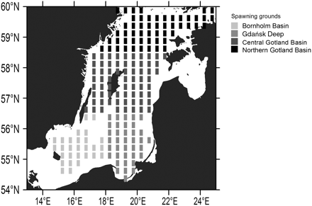
Data were primarily aggregated monthly for 10 m depth layers and for rectangles (representing quarters of ICES rectangles) of ∼15 × 15 nautical miles (Figure 1). To obtain life-stage-specific temperature trends, data about typical peak seasonal, as well as vertical abundance, were further aggregated over distribution ranges. Peak egg abundance was assigned to 50–60 m depth (ICES, 2010c) in May (Voss et al., 2006), with spawning being aggregated in the deep basins. Temperature trends were calculated separately for the three major spawning grounds (Bornholm Basin, Gdańsk Deep, Gotland Basin; Figure 1), as well as for the entire area (weighted by spawning ground size), by averaging temperature data in the specific depth intervals. Because sprat larvae and juveniles are distributed in the 0–10 m depth layer (Voss et al., 2007), we investigated whether there existed significant temperature trends in this depth layer in May (larvae) and August (juveniles). Because of the high drift and mixing potential (Hinrichsen et al., 2005; Baumann et al., 2006a), no sub-basin classification was applied for this life stage. We calculated decadal temperature trends by taking the slope from linear regression lines. These trends were tested for statistical significance.
Major sprat egg distribution areas (50–60 m depth) in the Baltic Sea. Rectangles indicate primary horizontal resolution; different shadings indicate aggregation to spawning grounds for later analysis.
Stock–recruitment models

The model revealed no violation of assumptions regarding the independence, homogeneity of variance, and normality of the residuals when checking the autocorrelation graphs and the Shapiro–Wilk normality test of residuals. The model explains more than 75% of the variance. The model was fitted to time-series 1979–2008, because BDAt is only available from 1979 on (Baumann et al., 2006a). We compared the fit of the model based on the Akaike information criterion (AIC) when using different temperature time-series: (i) May surface temperature based on satellite data (original model), (ii) May 0–10 m depth (larval distribution), (iii) August 0–10 m depth (older larvae/juveniles), and (iv) May 50–60 m depth (egg depth at peak spawning; aggregated data). AIC describes the predictive error of the model, thereby taking into account the fit, but also the model complexity (Burnham and Anderson, 2004). Terms that were no longer significant when using an alternative temperature time-series were removed from the model. For this comparison, the time-series had to be restricted to 1979–2005, because hydrodynamic model results were only available up to 2005.

Ecological–economic modelling
 .
. Parameters used in the ecological–economic model.
| Age class . | Maturity (ma) . | Weight (wa) (kg) . | Catchability (ϕa) . | Survival rate (ba) . | Numbers 1 April 2009 (109) . | Price ( € kg−1) . |
|---|---|---|---|---|---|---|
| 1 | 0.17 | 0.0053 | 0.31 | 0.6703 | 109.529 | 0.12 |
| 2 | 0.93 | 0.0085 | 0.54 | 0.7261 | 28.698 | 0.12 |
| 3 | 1.0 | 0.0097 | 0.76 | 0.7483 | 28.945 | 0.12 |
| 4 | 1.0 | 0.0103 | 1.0 | 0.7558 | 8.392 | 0.12 |
| 5 | 1.0 | 0.0108 | 1.0 | 0.7408 | 2.029 | 0.12 |
| 6 | 1.0 | 0.0112 | 1.0 | 0.7408 | 5.368 | 0.12 |
| 7 | 1.0 | 0.0113 | 1.0 | 0.7189 | 1.770 | 0.12 |
| 8 | 1.0 | 0.0110 | 1.0 | 0.7189 | 0.604 | 0.12 |
Parameters used in the ecological–economic model.
| Age class . | Maturity (ma) . | Weight (wa) (kg) . | Catchability (ϕa) . | Survival rate (ba) . | Numbers 1 April 2009 (109) . | Price ( € kg−1) . |
|---|---|---|---|---|---|---|
| 1 | 0.17 | 0.0053 | 0.31 | 0.6703 | 109.529 | 0.12 |
| 2 | 0.93 | 0.0085 | 0.54 | 0.7261 | 28.698 | 0.12 |
| 3 | 1.0 | 0.0097 | 0.76 | 0.7483 | 28.945 | 0.12 |
| 4 | 1.0 | 0.0103 | 1.0 | 0.7558 | 8.392 | 0.12 |
| 5 | 1.0 | 0.0108 | 1.0 | 0.7408 | 2.029 | 0.12 |
| 6 | 1.0 | 0.0112 | 1.0 | 0.7408 | 5.368 | 0.12 |
| 7 | 1.0 | 0.0113 | 1.0 | 0.7189 | 1.770 | 0.12 |
| 8 | 1.0 | 0.0110 | 1.0 | 0.7189 | 0.604 | 0.12 |
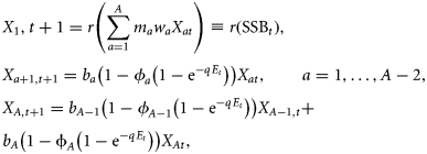
In Equation (3), Et denotes fishing effort in year t. In the following calculations, we choose units of effort such that the age-independent catchability parameter is normalized to unity, i.e. we set q= 1. Age-specific catchabilities (ϕa) were estimated based on mean age-specific fishing mortalities for 2007–2009 (FBAR 07–09), as reported in ICES (2010a), with ϕA = 1 for the oldest age class by normalization. With this specification of the harvesting function (Spence, 1973; Tahvonen, 2009), Et can be directly interpreted as the instantaneous fishing mortality that applies to the oldest age class.
Age-specific survival rates [ba = exp (−M2a)] were derived from predation mortality estimates (M2a values) as estimated by a stochastic multispecies model (SMS: Lewy and Vinther, 2004; ICES, 2010a) for the size of the cod stock in 2009 (ICES, 2010a). Age-specific maturity (ma), as well as age-specific weights (wa) used in Equation (3), were taken from single-species standard assessment (ICES, 2010a).


 to denote the discount factor, which can be calculated with the annual discount rate δ as
  .
.The term [1/(1−η)] formulates the fact that there is a broad aversion against large fluctuations in catches or income between years in the fishing industry. The higher the η, the more a constant income stream over time is preferred. Such a desire for relative constancy is reflected in several management plans for European fish stocks (e.g. Baltic cod; EU Commission, 2007), which have been agreed upon by a broad range of stakeholders, including fishers. For example, the formulation stipulates that TACs shall not change by more than a certain percentage between two subsequent years (15% for Baltic cod). For η= 0, the objective function, Equation (3), was simply the net present value of resource rents (or net revenues). In this study, results were calculated by applying a slightly non-linear objective function, η=0.1.
According to European legislation, sprat has only one marketing category, independent of age or size. Hence, the price p was the same for all age classes. Unit effort costs are denoted by c. Data availability did not allow an estimate of the unit effort cost for Baltic sprat. North Sea herring represents a stock similar to Baltic sprat in characteristics relevant to harvesting, i.e. a schooling pelagic fish that has a harvesting function available for unit effort cost (Bjørndal and Conrad, 1987; Nostbakken and Bjørndal, 2003; Nostbakken, 2008). In the following, we describe our approach of transferring the unit effort cost parameter for North Sea herring to our Baltic sprat model. Using a biomass model of North Sea herring, Bjørndal and Conrad (1987) estimated a catchability coefficient of qher-nsea,SSB= 0.0011 per vessel year. The relevant variable for the production function of a fishery is the concentration of fish (Clark, 1990, Chapter 7.6), which can be approximated as the current stock level divided by the carrying capacity (the unfished stock size). Nostbakken and Bjørndal (2003) estimated the carrying capacity of North Sea herring to be 5270 thousand tonnes.
When exerting zero fishing mortality in our age-structured population model, the parametrization yields a biomass of the unfished Baltic sprat stock of 1962 thousand tonnes. This can be interpreted as the carrying capacity of the Baltic Sea, which follows when applying our model specifications. Hence, for transferring the catchability parameter of North Sea herring to Baltic sprat, it has to be adjusted by the factor of 5270/1962≈2.69, which means that the same effort would result in a 2.69-fold higher fishing mortality for Baltic sprat than for North Sea herring. The catchability parameter for North Sea herring applies for the SSB, whereas in our model, it applies to the oldest age class. To adjust for this, we estimated the maximal fishing mortality relative to fishing mortality on SSB for Baltic sprat from ICES (2010a) data, obtaining a factor of 1.63 on average over the years 2006–2009. This results in a catchability parameter of q = 0.0011 × 2.69 × 1.63 = 0.0048 per vessel year. Nostbakken and Bjørndal (2003, Table 3) and Nostbakken (2008) report an average variable cost per vessel year of 1 189 656 NOK in 2001, which was equivalent to ∼0.15 million Euros. This yields a unit effort cost parameter of 0.15/0.0049 = 31.25 million Euros per unit of effort, where effort is measured in units of 1/q. To check for the influence of deviations from our cost estimate, we performed a sensitivity analysis for a broad range of cost estimates. The average price for sprat was, according to Finnish Statistics Yearbooks for 2004–2009 (Finnish Game and Fisheries Research Institute, http://www.rktl.fi/english/statistics/economy_and_the/producer_prices_for), 0.12 million Euros per 1000 t.
To determine the optimal management of the Baltic sprat, we numerically solved the optimization problem. For this, the dynamic optimization was performed using the interior-point algorithm of the Knitro (version 6.0) optimization software with Matlab (R2009b) and AMPL (A Modeling Language for Mathematical Programming, AMPL Optimization LLC, Albuquerque, USA).
Climate scenarios
Using this ecological–economic model, we investigated optimal management under two climate-change scenarios. These are based on International Panel on Climate Change (IPCC) emission scenarios A2 and B2 predicted using coupled regional atmospheric and hydrodynamic circulation models (BACC, 2008; Meier, 2006). The A2 scenario displays continually increasing emissions throughout the 21st century, whereas the B2 scenario displays an initial increase in emissions, which flattens from around 2050. These runs resulted in an increase in SST of 3.5 and 3°C, respectively, which are average projections for 2071–2100. We followed an approach of the Working Group on Integrated Assessments in the Baltic Sea (ICES, 2009b) to derive future temperature trends. In short, a time-series technique exploiting the autocorrelation pattern of the observed time-series was applied (Ripa and Lundberg, 1996) to create full-time trajectories of hydrographic variables. Time-series of future temperature were generated using the mean, variance, and autocorrelation structure of the historical time-series and a linear trend has been added to achieve the temperature values until 2100. Finally, to account for uncertainty in the predictions, a random noise component, based on the variation observed in 1973–2005, was added and 1000 future temperature time-series were generated and used for model forcing.
To estimate the potential impact of temperature change on optimal management results, the two climate-change scenarios were compared with a no-climate-change scenario, using the same mean, variance, and autocorrelation structure of the historical time-series, but without a trend added.
Results
Temperature trends
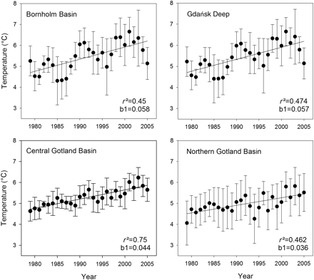
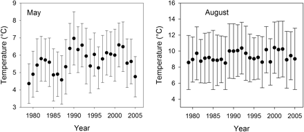
On all major spawning grounds, a significant (p< 0.01) temperature increase was recorded from 1979 to 2005 for the depth layer 50–60 m (Figure 2), which is most relevant for floating sprat eggs. The amount of temperature increase decreases from the Bornholm Basin to the Northern Gotland Basin, i.e. from southwest to northeast. Linear regression analysis estimated that the total temperature increase was ∼0.9°C (Northern Gotland Basin) to 1.5°C (Bornholm Basin) over the observation period. Despite the overall positive temperature trend, within-area variability (as measured by the standard deviation), as well as year-to-year variability, was high. Lowest variability was found for both components in the central Gotland Basin, where the fit of the linear regression was best. In all other areas, the general warming trend was partly masked by year-to-year variability because of additional effects. In the surface layer (0–10 m depth; Figure 3), the regressions were not significant (p> 0.05). Within-area variability was large. Year-to-year variation was more pronounced in May than August, and was stronger than the underlying warming trend.
Temperature trend in the depth layer 50–60 m from 1979 to 2005, for four major sprat spawning grounds in the Baltic Sea (see Figure 1). Area means are provided, along with standard deviations and the results of linear regression analysis (fit: r²; slope: b1).
Temperature trend in the surface layer 0–10 m depth from 1979 to 2005, for the complete Central Baltic in May (left) and August (right). Area means are provided along with standard deviations.
Stock–recruitment relationships
Using the alternative temperature time-series (1979–2005) as determined by hydrodynamic modelling did not improve the fit of the stock–recruitment function (Table 2). Out of the three tested variants, temperature at 0–10 m depth in August had the highest explanatory power (AIC = 20.3), but still explained less variance than the satellite data for May surface temperature (AIC = 18.65). When including density-dependence in the recruitment model (Table 3), temperature at 0–10 m depth in August, as derived from the hydrodynamic model, explained most of the variability. However, the differences in model fit using original, or new, model-based temperature datasets were rather small, compared with the difference that existed depending on whether or not data for the past 3 years were included. Overall, models including density-dependence had slightly higher AIC values.
Fit of sprat recruitment model (as estimated by ICES, 2010b), using different temperature time-series (SST).
| Model number . | Temperature source (SST) . | Years . | AIC . | Insignificant variables . |
|---|---|---|---|---|
 | ||||
| 1 | SAT-May (original model) | 1979–2008 | 30.67 | |
| 2 | SAT-May | 1979–2005 | 18.65 | BDA3 |
| 3 | 0–10 m Augusta | 1979–2005 | 20.3 | SST2 |
| 4 | 0–10 m Maya | 1979–2005 | 25.75 | SST2; BDA3 |
| 5 | 50–60 m Maya | 1979–2005 | 25.64 | BDA3 |
| Model number . | Temperature source (SST) . | Years . | AIC . | Insignificant variables . |
|---|---|---|---|---|
 | ||||
| 1 | SAT-May (original model) | 1979–2008 | 30.67 | |
| 2 | SAT-May | 1979–2005 | 18.65 | BDA3 |
| 3 | 0–10 m Augusta | 1979–2005 | 20.3 | SST2 |
| 4 | 0–10 m Maya | 1979–2005 | 25.75 | SST2; BDA3 |
| 5 | 50–60 m Maya | 1979–2005 | 25.64 | BDA3 |
Variables turning insignificant when using alternative time-series are indicated; SSB, spawning-stock biomass; SST, temperature; BDA, bottom depth anomaly; SAT-May, sea surface temperature in May as derived by satellite data; 0–10 m August, temperature in 0–10 m depth in August; 0–10 m May, temperature in 0–10 m depth in May; 50–60 m May, temperature in 50–60 m depth in May.
aData from hydrodynamic model.
Fit of sprat recruitment model (as estimated by ICES, 2010b), using different temperature time-series (SST).
| Model number . | Temperature source (SST) . | Years . | AIC . | Insignificant variables . |
|---|---|---|---|---|
 | ||||
| 1 | SAT-May (original model) | 1979–2008 | 30.67 | |
| 2 | SAT-May | 1979–2005 | 18.65 | BDA3 |
| 3 | 0–10 m Augusta | 1979–2005 | 20.3 | SST2 |
| 4 | 0–10 m Maya | 1979–2005 | 25.75 | SST2; BDA3 |
| 5 | 50–60 m Maya | 1979–2005 | 25.64 | BDA3 |
| Model number . | Temperature source (SST) . | Years . | AIC . | Insignificant variables . |
|---|---|---|---|---|
 | ||||
| 1 | SAT-May (original model) | 1979–2008 | 30.67 | |
| 2 | SAT-May | 1979–2005 | 18.65 | BDA3 |
| 3 | 0–10 m Augusta | 1979–2005 | 20.3 | SST2 |
| 4 | 0–10 m Maya | 1979–2005 | 25.75 | SST2; BDA3 |
| 5 | 50–60 m Maya | 1979–2005 | 25.64 | BDA3 |
Variables turning insignificant when using alternative time-series are indicated; SSB, spawning-stock biomass; SST, temperature; BDA, bottom depth anomaly; SAT-May, sea surface temperature in May as derived by satellite data; 0–10 m August, temperature in 0–10 m depth in August; 0–10 m May, temperature in 0–10 m depth in May; 50–60 m May, temperature in 50–60 m depth in May.
aData from hydrodynamic model.
Fit of sprat recruitment model (as estimated by ICES, 2010b, and including density-dependence), using different temperature time-series (SST).
| Model number . | Temperature source (SST) . | Years . | AIC . | Insignificant variables . |
|---|---|---|---|---|
 | ||||
| 6 | SAT-May (original model) | 1979–2008 | 34.87 | |
| 7 | SAT-May | 1979–2005 | 23.37 | BDA3 |
| 8 | 0–10 m Augusta | 1979–2005 | 20.77 | SST2 |
| 9 | 0–10 m Maya | 1979–2005 | 29.1 | SST2 |
| 10 | 50–60 m Maya | 1979–2005 | 29.8 | SST2 |
| Model number . | Temperature source (SST) . | Years . | AIC . | Insignificant variables . |
|---|---|---|---|---|
 | ||||
| 6 | SAT-May (original model) | 1979–2008 | 34.87 | |
| 7 | SAT-May | 1979–2005 | 23.37 | BDA3 |
| 8 | 0–10 m Augusta | 1979–2005 | 20.77 | SST2 |
| 9 | 0–10 m Maya | 1979–2005 | 29.1 | SST2 |
| 10 | 50–60 m Maya | 1979–2005 | 29.8 | SST2 |
Variables turning insignificant when using alternative time-series are indicated; SSB, spawning-stock biomass; SST, temperature; BDA, bottom depth anomaly; SAT-May, sea surface temperature in May as derived by satellite data; 0–10 m August, temperature in 0–10 m depth in August; 0–10 m May, temperature in 0–10 m depth in May; 50–60 m May, temperature in 50–60 m depth in May.
aData from hydrodynamic model.
Fit of sprat recruitment model (as estimated by ICES, 2010b, and including density-dependence), using different temperature time-series (SST).
| Model number . | Temperature source (SST) . | Years . | AIC . | Insignificant variables . |
|---|---|---|---|---|
 | ||||
| 6 | SAT-May (original model) | 1979–2008 | 34.87 | |
| 7 | SAT-May | 1979–2005 | 23.37 | BDA3 |
| 8 | 0–10 m Augusta | 1979–2005 | 20.77 | SST2 |
| 9 | 0–10 m Maya | 1979–2005 | 29.1 | SST2 |
| 10 | 50–60 m Maya | 1979–2005 | 29.8 | SST2 |
| Model number . | Temperature source (SST) . | Years . | AIC . | Insignificant variables . |
|---|---|---|---|---|
 | ||||
| 6 | SAT-May (original model) | 1979–2008 | 34.87 | |
| 7 | SAT-May | 1979–2005 | 23.37 | BDA3 |
| 8 | 0–10 m Augusta | 1979–2005 | 20.77 | SST2 |
| 9 | 0–10 m Maya | 1979–2005 | 29.1 | SST2 |
| 10 | 50–60 m Maya | 1979–2005 | 29.8 | SST2 |
Variables turning insignificant when using alternative time-series are indicated; SSB, spawning-stock biomass; SST, temperature; BDA, bottom depth anomaly; SAT-May, sea surface temperature in May as derived by satellite data; 0–10 m August, temperature in 0–10 m depth in August; 0–10 m May, temperature in 0–10 m depth in May; 50–60 m May, temperature in 50–60 m depth in May.
aData from hydrodynamic model.
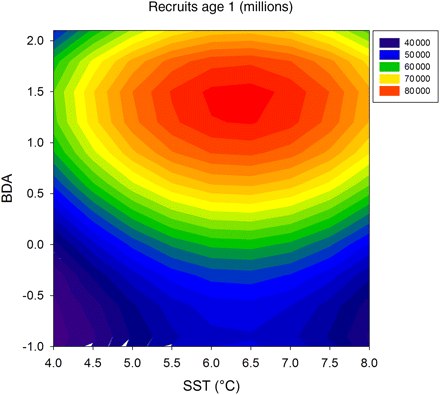
We assumed density-dependence in our modelling approach and used model number 7 (Table 3), i.e. the model giving the second best fit for this kind of stock–recruitment function (Table 3). We did not use model 8 (best fit), because temperature projections under climate-change scenarios are currently only available for satellite-derived surface temperature and not for any other water depth (Meier, 2006; BACC, 2008). We estimated the effect of variation in environmental conditions (SST and BDA) on recruitment strength (Figure 4). In these calculations, SSB was maintained at 800 000 t. In the range of historically observed variability, maximum recruitment was reached at ∼6.3°C sea surface temperature in May and a BDA of 1.4 (indicative of retention of larvae within spawning grounds). Because changes in BDA cannot currently be forecast, we used the average value in 1979–2008 for further computations (BDA = 0.096).
Sprat recruitment strength (age 1) in dependence of sea surface temperature in May (SST) and bottom depth anomaly (BDA, representing larval drift). Recruitment per SSB is calculated according to the formula:  .
.
Optimal management of the Baltic sprat stock
Time-trajectory under no climate change
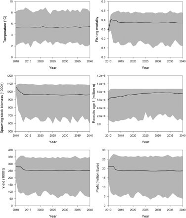
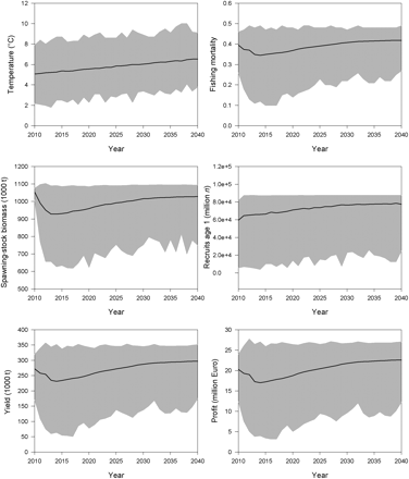
The time-trajectory assuming no positive trend in temperature demonstrated that the largest year-to-year changes in F, SSB, yield, and profit happened in the first 5 years of the simulation (Figure 5). Already after 5 years, i.e. in 2015, a stable steady state is reached. Mean optimal fishing mortality rapidly adjusted from <0.3 in the first year of the simulation (2010) to 0.39 in the steady state. Small deflections in the trajectories during transition to the steady state are attributed to the initial age structure. The long-term mean optimal size of the SSB is estimated at ∼970 000 t, with an annual catch of ∼250 000 t and an estimated profit of ∼19 million Euros. There is a broad range of possible solutions that depend on variability in the 1000 temperature time-series iterations. Because the recruitment function has a maximum at ∼6.3°C and because it is density-dependent, there is an upper bound, which is regularly reached. The existence of an upper limit in the recruitment function resulted in a skewed distribution of possible outcomes around the mean. This skewed distribution in recruitment caused skewed distributions also in the results on F, SSB, yield, and profit.
Maximizing net revenue from the Baltic sprat stock: model results of 1000 temperature time-series iterations, assuming no climate change. Mean values (black lines) are given along with a range of possible solutions (grey area).
Effect of SST and BDA
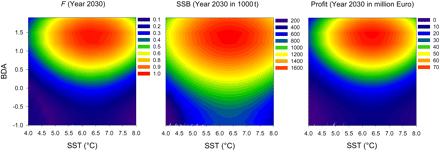
We investigated optimal management for a range of combinations of SST and BDA values that were held constant over time. The general shape is the same for fishing mortality, SSB, and profit (Figure 6). Highest values were calculated for a combination of environmental conditions that were most favourable for recruitment. After 20 years of simulation, i.e. when a steady state was reached after the initial adjustment period, instantaneous fishing mortality rates varied between 0.1 and 1. Only under a permanent state of optimal environmental conditions could values as high as 1 be reached. For the long-term mean values of BDA and SST, an optimal fishing mortality of ∼0.39 would result from the simulations (see also Figure 5). Therefore, SSB levels vary between 200 000 t and 1.6 million t, whereas profits range between 0 and 70 million Euros per year.
Ecological–economic optimization for a range of SST and BDA values: Results after 20 years modelling time, i.e. after reaching the steady state, are given for instantaneous fishing mortality (F; left panel), SSB (middle panel), and profit (right panel).
Effect of costs and interest rate
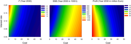
Variations in fishing costs have a large impact on the optimal solution (Figure 7). As could be expected, rising costs generally resulted in lower fishing mortalities and associated higher SSB values, but lower profits. In the extremes, fishing mortality ranged from 0.22 (high costs and small interest rate) to 1.27 (zero costs and high interest rate). Variation in interest rate had only minor impact at a cost parameter of 31.25, our best-guess estimate, but became important at very small cost estimates.
Ecological–economic optimization for a range of cost (unit effort cost parameter) and interest rate values. Results after 20 years modelling time, i.e. after reaching the steady state, are given for instantaneous fishing mortality (F; left panel), SSB (middle panel), and profit (right panel).
Climate-change scenarios
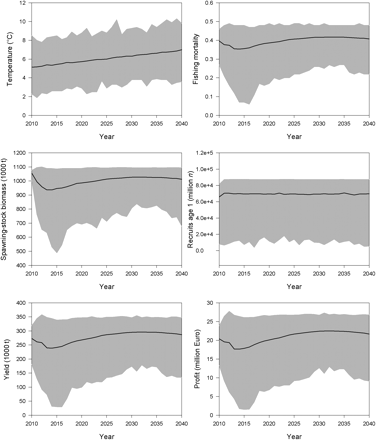
Using the climate-change scenarios A2 (Figure 8) and B2 (Figure 9) resulted in quite similar solutions. As for the no-climate-change scenario, the largest year-to-year changes occurred in the first 5 years. However, the period needed to achieve a (relatively) stable state was considerably longer. Over a long period, fishing mortality did not reach a fixed value, but steadily increased with temperature increase. After an initial decline, optimal SSB was calculated to be larger than in the no-climate-change scenario, i.e. >1 million tonnes in both scenarios. At the beginning of the simulation, mean yields and profits were somewhat lower, but reached higher values at the latest in 2020. Maximizing net revenues resulted in mean profits in 2030, which were >18% higher in the A2 scenario than in the no-climate-change scenario (15% for B2 scenario). At the start of the simulation, as well as after reaching the (relatively) steady state after 25 years, all output components (SSB, recruitment, F, yield, and profit) were statistically different between the no-climate-change scenario and scenarios A2 and B2 (Table 4). The two scenarios assuming climate change were, however, never statistically different (p> 0.05). After only 5 years of simulation, some statistical differences were noted (Table 4).
Results of statistical analysis (F-test), comparing outcomes of different climate-change scenarios.
| Years . | Scenario . | SSB . | Recruitment . | F . | Yield . | Profit . |
|---|---|---|---|---|---|---|
| 2 | NO-A2 | *** | *** | *** | *** | *** |
| 2 | NO-B2 | *** | *** | *** | *** | *** |
| 2 | A2-B2 | n.s. | n.s. | n.s. | n.s. | n.s. |
| 5 | NO-A2 | *** | n.s. | ** | * | n.s. |
| 5 | NO-B2 | *** | * | *** | *** | *** |
| 5 | A2-B2 | n.s. | n.s. | ** | * | n.s. |
| 25 | NO-A2 | *** | *** | *** | *** | *** |
| 25 | NO-B2 | *** | *** | *** | *** | *** |
| 25 | A2-B2 | n.s. | n.s. | n.s. | n.s. | n.s. |
NO, no climate change; A2, climate-change scenario A2; B2, climate-change scenario B2; SSB, spawning-stock biomass; F, fishing mortality; n.s., not significant.
*p<0.05; **p< 0.01; ***p< 0.001.
Maximizing net revenue from the Baltic sprat stock: model results of 1000 temperature time-series iterations, assuming climate change under the A2 scenario. Mean values (black lines) are given along with a range of possible solutions (grey area).
Maximizing net revenue from the Baltic sprat stock: model results of 1000 temperature time-series iterations, assuming climate change under the B2 scenario. Mean values (black lines) are given along with a range of possible solutions (grey area).
Discussion
This study examined how the effect of climate-change-induced temperature increase can be examined using an ecological–economic model of a fishery harvesting an age-structured fish population. For Baltic sprat, we illustrated how to combine field observations of temperature increase and stock–recruitment modelling to estimate optimal management strategies in dependence of economic factors and climate-change scenarios. Optimal management strategies, in our terminology, maximize a societal objective function that takes into account the benefits (i.e. the economic value of the yield) and the costs of fishing. We considered an explicitly dynamic framework, where current reductions in profit (which are necessary to rebuild the currently overfished stock) are pitted against higher future profits from fishing. The effects of fishing and climate-change on the stock were taken into account as dynamic constraints in the optimization.
Only a few studies have tried to quantify the economic consequences of climate change for fisheries. These include an analysis of the stability of fishery agreements under climate change (Brandt and Kronbak, 2010) or the fisheries impact of global warming on the Icelandic and Greenland economy (Arnason, 2007). A comparison of harvesting strategies under climate change (here: changes in the strength of the Atlantic thermohaline circulation) was provided by Link and Tol (2009) for the Barents Sea fisheries. They demonstrated that environmentally induced changes in recruitment success could cause the associated fisheries to become unprofitable and argue for a more flexible harvest strategy to deal efficiently with climate-change effects on fisheries.
Using Baltic sprat as an example of how to approach ecological–economic modelling of a fishery under climate change had several advantages because of data availability and process understanding. The three-dimensional ocean circulation model of the Baltic Sea used here to determine ambient temperatures of sprat early-life-history stages has been well corroborated and provides a coherent picture of the circulation, water mass exchange, and physical properties within the Baltic Sea (Lehmann and Hinrichsen, 2000; Meier et al., 2006). The large within-area temperature variability observed demands a more detailed investigation of mesoscale spatial processes which, however, was not a focus of the current study. Using temperature estimates for August at 0–10 m depth enhanced the recruitment prediction when assuming density-dependence. This agrees with earlier studies, which highlighted the importance of larval and juvenile stages for Baltic sprat recruitment (Baumann et al., 2006a; Voss et al., 2006).
A better spatial representation of egg and larval/juvenile distributions before averaging ambient temperature could improve the estimates and result in a more pronounced enhancement of the fit of temperature-dependent stock–recruitment functions. However, prognostic simulations with the circulation model of the Baltic Sea are unavailable. Therefore, surface temperature data were used, for which climate-change scenarios were available (ICES, 2010b).
Factors contributing to variations in recruitment strength are crucial for management considerations and stock projections (ICES, 2009c). In Baltic sprat, recruitment variation is largely influenced by environmental conditions (Baumann et al., 2006a; Voss et al., 2006). Environmentally sensitive stock–recruitment relationships were partially formulated by previous investigators (Köster et al., 2003; MacKenzie and Köster, 2004; Margonski et al., 2008), but those relationships did not include SSB and also utilized non-predictable environmental variables (i.e. January–February NAO index, MacKenzie and Köster, 2004). The fit of the models could be enhanced further using regionalized variables, such as the BDA (Baumann et al., 2006a), which are related to some degree to the NAO index, but remain unpredictable. These shortcomings made those models unsuitable for economic optimization purposes under climate-change scenarios. In this study, we used the most recent formulation of environmental dependence, including surface temperature as a predictable and BDA as an unpredictable variable (ICES, 2010b), as well as density-dependence of the spawning stock. A sensitivity analysis indicated that the model was influenced by different values of BDA; hence, for the climate-change scenarios, the average long-term value was employed. If climate change would, however, result in more frequent, stronger wind-driven larval transport to the coast, such changes in BDA could counteract the positive effect of temperature increase on sprat recruitment. The assumption of density-dependence in the stock–recruitment function seems reasonable, because sprat are cannibalistic (Köster and Möllmann, 2000a) and exhibit food competition (Casini et al., 2006, 2010). The available time-series of stock and recruit data do not indicate reduced recruitment at higher stock sizes (ICES, 2010a); however, these might be reached under an economic optimization setup. Although incorporating environmental forcing, the recruitment model does not capture irregularly appearing very strong year classes of sprat (ICES, 2010a). Therefore, the use of a stochastic stock–recruitment model is one challenge in our future work. This emphasizes the need for further coupled investigations of temperature change, ocean circulation, and recruitment dynamics in the Baltic to permit formulating effective harvest control rules.
In contrast to an MSE approach, our approach considers a one-dimensional objective (the current value of profits from fishing) rather than multiple criteria. In this respect, our approach is closely related to an economic cost–benefit analysis. Rather than considering one or a few management strategies, however, the optimization approach determines the optimal management strategy out of an infinite number of possibilities.
Given the rather strong assumptions, the results of this approach should be interpreted as an example of how to apply the method, rather than as a concrete proposal for a new management approach for the Baltic sprat fishery (such as the HCR proposed by ICES 2009c, d). Because of missing data, we had to transfer an economic parameter from the North Sea herring fishery to Baltic sprat, i.e. the unit effort cost parameter. The most relevant variable for the production function is the concentration of fish, which was approximated by the current stock level divided by the carrying capacity, thereby not explicitly taking into account area size. This approach assumes that catchabilities and vessel costs in North Sea herring and Baltic sprat fishery are the same. Herring is one of the best-studied examples in fisheries economics (Bjørndal and Conrad, 1987; Nostbakken and Bjørndal, 2003; Nostbakken, 2008) and is similar to sprat in characteristics relevant for fishing. Moreover, no ecological interactions, e.g. competition between sprat and herring stocks, or other feedbacks were incorporated into the model, although such relationships do exist (Casini et al., 2006, 2010). The only exception was cod predation on sprat, which was included in SMS, the most recent Baltic Sea multispecies model (Lewy and Vinther, 2004; ICES, 2010a). Changes in Baltic cod stock size, such as the successful rebuilding of this major predator stock to levels in the 1980s, would certainly influence our results both directly, via effects on natural mortality and therefore sprat stock size, as well as indirectly via changed unit effort costs because of lower concentrations of sprat (unpublished data).
Our simulations used a slightly non-linear objective function, η = 0.1. For a linear objective function (η = 0), the optimal outcome would be pulse fishing, i.e. intermittent high catches during one period interrupted by one or more periods with zero or very low catches. The annual mean catches have been demonstrated to be only slightly higher (<1%) than the non-pulse fishing solution, given η = 0.1. For η > 0.1, the long-term steady state was not influenced by increasing η, but the transition period towards the steady state was longer.
The goal of future work will be to provide appropriate multispecies management advice that includes economic considerations in a variable or changing environment. Under the current knowledge of Baltic sprat recruitment, the tested climate-change scenarios would result in a change in management targets. To serve as a quantitative management advice tool, however, the model will have to address the above-mentioned concerns.
Acknowledgements
We thank two anonymous reviewers and especially Anna Gårdmark for valuable comments on a first draft, which considerably improved the manuscript. The study was carried out with financial support from the Cluster of Excellence “Future Ocean” of Kiel University and from the European Communities as a contribution to the FP7 Specific Targeted Research Project 244966, Forage Fish Interactions (FACTS). This article does not necessarily reflect the views of the European Commission.


