Intrastock differences in maturation schedules of Atlantic cod, Gadus morhua

Abstract

Wright, P. J., Millar, C. P., and Gibb, F. M. 2011. Intrastock differences in maturation schedules of Atlantic cod, Gadus morhua. – ICES Journal of Marine Science, 68: 1918–1927.

Differences in maturation schedules from three subpopulations of North Sea cod (Gadus morhua) were examined using the demographic probabilistic maturation reaction norm (PMRN) approach. Declines in maturation probability with size and age were evident within the North Sea cod stock, but the magnitude of decline differed among subpopulations. The difference in the rate of decline led to significant spatial differences in recent times. Changes in maturation probability could not be explained by colonization from adjacent regions indicating a local response to conditions. The greatest decline in maturation probability followed the near collapse of regional spawning biomass during the 1980s and 1990s. A new methodology was developed to integrate the effects of temperature and competitive biomass into the estimation of the PMRN. Temperature had a positive effect on maturation probability, but could only partially explain the decreasing trend in PMRN midpoints. Consequently, regional selection for early maturing genotypes provides the most parsimonious explanation for the declines in maturation probability observed. The difference in maturation probability among North Sea cod subpopulations, and the additive contribution of temperature to the estimation of change, underscores the need to account for population structuring and to incorporate temperature as a covariate in future applications of the PMRN.

Introduction

Marked declines in size and age at maturity have been reported widely in many exploited fish stocks (Law, 2000; Jørgensen et al., 2007). Such changes in maturation schedules may arise from the reduced intraspecific competition associated with a declining stock, because fish growing faster will attain the size and condition required for maturation at an earlier age (Trippel, 1995; Grift et al., 2007). However, such a compensatory response does not explain why there is often a downward shift in the size-at-age trajectory of maturity. Indeed, in some cases, earlier maturation has been associated with a reduction in growth and condition (Morgan et al., 1994; Yoneda and Wright, 2004). Genetic selection has been implicated in such shifts in the size and age at maturity, because there is a heritable component to both (Gjerde, 1984). Fishing is probably an important contributing factor to this genetic change (Trippel, 1995; Law, 2000; Jørgensen et al., 2007) because the mortality it imposes can be considerably greater than natural mortality (Olsen and Moland, 2011) and may even change the pattern of selection from juveniles to adults (Conover, 2007). Life-history theory predicts that such changes in mortality schedules should select for earlier maturation, increased reproductive investment, and a change in growth rate (Roff, 1992; Law, 2000).

There is little direct genetic evidence for changes in maturation schedules, and attempts to identify such a response have looked for trends in traits that appear to counter that predicted from plastic responses alone (i.e. counter-trend variation; Dieckmann and Heino, 2007). Most such indirect evidence has come from applications of the probabilistic maturation reaction norm (PMRN) that describes the probability of immature fish maturing at a certain age and size (Heino et al., 2002) and condition (Grift et al., 2007). This maturation probability is expected to be independent of the variations in growth and mortality that confound descriptions of change based on maturity ogives. Nevertheless, interpretation of trends in PMRN reaction norm midpoints requires caution, because the method can be confounded by unaccounted for environmental influences on maturation, such as the growth-independent effect of temperature on the maturation-decision process (Dhillon and Fox, 2004; Tobin and Wright, 2011). Past studies have only considered the significance of such environmental influences from an analysis of the Lp50 cohort regression (e.g. Mollet et al., 2007). However, incorporating environmental factors into the estimation of PMRN, in addition to cohort, is the only statistically sound approach to the identification and disentanglement of additional plastic effects on maturation (Dieckmann and Heino, 2007). Moreover, as field applications are limited by a need to characterize gonad development macroscopically, reported midpoints reflect the energetic outcome of the continued gonadal development of a fish rather than its state when the physiological decision to continue gametogenesis was made (Wright, 2007).

The Atlantic cod (Gadus morhua) has been central to the debate over fisheries-induced genetic selection of life-history traits, because there have been rapid declines in PMRN reaction midpoints in some of the most heavily exploited stocks, such as the northern (Olsen et al., 2004) and Georges Bank (Barot et al., 2004a) populations. Like a number of marine fish species, stocks of Atlantic cod often consist of both resident and migratory subpopulations (Wright et al., 2006; Righton et al., 2007; Olsen et al., 2008). The North Sea cod stock was once one of the most productive (Brander, 1994), but is now highly depleted (ICES, 2009), with most of it now concentrated in the northern North Sea (Hedger et al., 2004; ICES, 2009). Studies of maturity in this stock have demonstrated that the mean age at first maturity has declined considerably over the past century (Holt, 1893; Oosthuizen and Daan, 1974; Rijnsdorp et al., 1991; Yoneda and Wright, 2004). More recently, Yoneda and Wright (2004) showed that since the last period of high spawning-stock size in the late 1960s, spatial differences in reproductive investment have developed, with cod from the northwest inshore (NW) region of the North Sea now maturing smaller and having a greater fecundity than those in the deeper northeastern North Sea. Differences in maturity at size were also detected between cod from this NW region and the southern (S) North Sea in both the field and under a common environment (Harrald et al., 2010). These regional differences in maturity reflect spatially (Wright et al., 2006; Righton et al., 2007) and genetically segregated spawning populations of the species in the North Sea (Hutchinson et al., 2001; Nielsen et al., 2009). Given regional differences in sea temperature and its recent rate of warming (Elliot et al., 1991; Sharples et al., 2006), the spatial pattern of maturation in the North Sea may reflect counter-gradient selection, fish tending to mature smaller in order to compensate for a less-favourable environment (Conover et al., 2006). Conversely, as North Sea fisheries targeting cod have tended to move from coastal to offshore waters over the past five decades (Jennings et al., 1999; Greenstreet et al., 2009), the current spatial variability in life-history traits could reflect divergent responses to local selective pressures. Any analysis of temporal changes in reproductive investment should therefore be considered in relation to population structure and environmental forcing, because failure to account for an appropriate spatial scale could lead to erroneous conclusions on the magnitude of the change.

In this study, trends in maturation schedules from three subpopulations of North Sea cod were examined using the demographic PMRN approach (Barot et al., 2004b). As maturation appears to be influenced by the state of the fish during critical periods of the year (Wright, 2007), which may in turn be influenced by temperature (Dhillon and Fox, 2004), trends in PMRN were examined in relation to the biomass of conspecifics and bottom sea temperature around the summer maturation decision phase (Davie et al., 2007). A methodology was developed to integrate these potential explanatory influences into the estimation of the PMRN. Unexplained trends in reaction norm midpoints were then considered in relation to predictions about genetically induced changes in life-history traits.

Material and methods

Data on sex, maturity, age, and length were extracted from the first quarter ICES (International Council for the Exploration of the Sea) International Bottom Trawl SMALK (sex–maturity–age–length keys) database (DATRAS), for the years 1971–2009. These bottom trawl surveys were undertaken between January and March, i.e. within 1 month of cod spawning (Hislop, 1984). The data were supplemented with additional research and commercial trawl sampling in the years 1999, 2002–2004, and 2008. Total length was measured to the nearest 1 cm, and maturity stage was determined macroscopically as either two stages before 1990 or four stages after 1990: 1, immature; 2, developing; 3, spawning; 4, spent. All data were segregated into three regions corresponding to putative subpopulations from the S, NW, and northeast offshore (NE) North Sea (Figure 1; see Hutchinson et al., 2001; Nielsen et al., 2009). Table 1 summarizes the number-at-age for each subpopulation and cohort. Data sparseness was a problem for age 3+ cod from the NW and S, with many cohorts having <100 individuals per age class. As SMALK data were from a length-stratified sampling programme, annual length increments between ages 1 and 4 caught in research bottom trawls were estimated from age-stratified length frequency compositions raised to catch per hour from the DATRAS database.

Table 1.

Number of cod at age (1–4) for each North Sea region (northeast, NE; northwest inshore, NW; southern, S), and the mean number per cohorts, 1976–2005.

		Age (years)
Region	Data type, cohorts	1	2	3	4	Total	% female aged 2–4
NE	Total, 1976–2005	168	2 310	2 061	1 092	5 631	49.5
	Mean per cohort	6	80	71	37	–	–
NW	Total, 1977–2005	2 001	2 641	1 330	454	6 426	46.0
	Mean per cohort	71	94	48	16	–	–
S	Total, 1976–2005	1 392	4 190	1 262	258	7 398	49.0
	Mean per cohort	48	144	43	9	–	–

Figure 1.

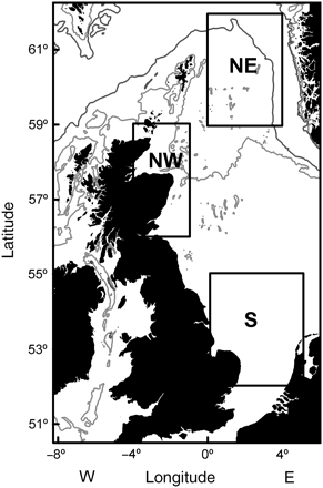
Location of the three regions of North Sea cod Gadus morhua (northeast, NE; northwest, NW; southern, S), indicated by solid lines. Dark grey and light lines represent the 200 and 100 m depth contours, respectively.

PMRN estimation

Two methods were applied to estimate the PMRN. As the data do not distinguish between first time and repeat spawners, the retrospective demographic PMRN method developed by Barot et al. (2004b) was used to permit comparison with previous studies. To consider possible environmental influences on the PMRN, an alternative approach was also applied, based on the ideas of survival analysis (Cox, 1972), which uses auxiliary information on growth plus other covariates, such as temperature, to reconstruct the full life history. This approach is referred to as the life-history PMRN model, and is similar in spirit to that presented by Van Dooren et al. (2005) and Kuparinen et al. (2008). Both models were fitted with Bayesian methods, using priors designed to give good frequentist properties. Model selection was based on t likelihood, using minimum Bayesian information criteria (BIC), and significance of terms was assessed using the likelihood ratio statistic. The demographic PMRN approach of Barot et al. (2004b) is presented along with the life-history PMRN model.

The retrospective demographic PMRN approach of Barot et al. (2004b) requires (for each sex, cohort, and subpopulation) estimates of the probability of being mature at each age a and size s, and estimates of the increase in size over the previous year, ⁠, of a fish that is currently at age a and size s. The difference is the probability that a fish of age a and size s matures at age a. Scaling by the probability that the fish is immature at age a–1 gives the probability of maturing at age a, conditional on being immature the previous year:

(1)

For each age a, the PMRN midpoint (or Lp50) is the size s at which m(a, s) = 0.5. The method assumes that immature and mature fish have the same rates of survival and growth; however, PMRN estimates are relatively robust to a relaxation of this assumption (Barot et al., 2004b).

Maturity ogives were estimated by logistic regression of individual maturity state (immature or mature) on length, age, sex, cohort, and subpopulation, and their interactions, with age and cohort treated as categorical variables. There were insufficient data to fit a full model, i.e. to estimate a separate maturity ogive for each combination of age, sex, cohort, and subpopulation, so a more parsimonious model was sought. This was chosen by forward and backward stepwise selection using the BIC to penalize models with many parameters. The final model was

(2)

which has a different slope (length effect) for each combination of age and subpopulation, and a different intercept for each combination of age and subpopulation, and each sex. Maturity ogive estimation was limited to ages at first maturity, i.e. 2–4, so requiring cod of age 1 to estimate growth increments.

Annual increases in size were estimated by fitting the growth model:

(3)

on the log link and assuming γ errors with constant coefficient of variation (CV), where l denotes length, a the age, and (the log mean length-at-age 1) and (a parameter that modifies the growth rate) are specific parameters of cohort, c, and subpopulation, r. Numbers at length were weighted by the catch per hour. Based on this model, the length in the previous year of an age a and length l fish was estimated to be ⁠, giving size increments

(4)

Inference about the Lp50 estimates is non-trivial, because the estimates are complicated functions of the maturity ogive and growth model parameter estimates, and are correlated because of the structure of the ogive model [Equation (2)]. Other authors (e.g. Barot et al., 2004a, b) have conditioned on the growth increments and used bootstrap methods and randomization tests to make inferences about PMRN and Lp50. A Bayesian approach was used here because it provides a more direct method to making inferences about a variety of PMRN quantities, including Lp50s. The attractiveness of the approach is its simplicity: given a draw from the posterior distribution of the ogive model parameters, and a draw from the posterior distribution of the growth model parameters, then assuming that the growth model is independent of the maturity model, a draw from the posterior distribution of any function of these parameters is computed easily, for example, an Lp50, or the slope between two Lp50s.

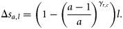
Markov chain Monte Carlo methods (MCMC; Gelman and Carlin, 2004) were used to sample from the posterior distribution of the growth and maturity model parameters. Specifically, single block update random walk Metropolis–Hastings algorithms were used where the variance matrix of the random walk was ⁠, being the variance matrix of the associated maximum likelihood estimates (attainable from standard software) and n the dimension of ⁠; an additional row and column was added to for the log CV of the growth model, which was assumed to be independent of all other estimates. The random walk is design to provide the chain optimal properties (Gelman and Carlin, 2004). Both chains were initiated at the maximum likelihood estimates and ran for 5000 iterations as a burn in, after which every fifth iteration was recorded to remove autocorrelation, until 1000 samples had been obtained. Credible intervals (the Bayesian equivalent of confidence intervals) for the Lp50s were then obtained as the 2.5th and 97.5th percentiles of the simulated distributions of each Lp50.

The posterior distributions were also used to test for an effect of sex or subpopulation on Lp50 and for a trend in Lp50 with cohort. The sex effect was measured by the mean difference in Lp50 between males and females, averaged across ages, cohorts, and subpopulations. A 95% credible interval for the mean difference was computed from the posterior distribution of the Lp50s, with sex having a significant effect if zero lay outside the credible interval. Similarly, the subpopulation effect was tested by calculating a two-dimensional 95% credible region for the mean differences in Lp50 (averaged across ages, cohorts, and sexes) between the NE and NW subpopulations, and between the NW and S subpopulations, and examining whether zero lay within that region. Finally, cohort trends in Lp50 for each sex, age, and subpopulation were assessed by smoothing the estimates of Lp50s and calculating the difference in the smoothed values Lp₁ and Lp₂ at the start and end of the time-series (1979 and 2005, corresponding to the shortest time-series). Again, a 95% credible interval was computed for this difference.

In addition, the magnitude of change was calculated as

(5)

and the apparent rate of evolutionary change, in the standard unit “darwin”, was calculated as

(6)

Incorporating explanatory variables in the estimation of maturation probability

Environmental covariates were integrated into the estimation of PMRN, in addition to cohort, because this is the only statistically sound approach to the identification and disentanglement of additional plastic effects on maturation (Dieckmann and Heino, 2007). One solution to achieving this is to model the probabilities of maturing and to use these estimates to build a cumulative probability of maturation to test against data. This is related to the approach taken by Van Dooren et al. (2005) and Kuparinen et al. (2008), in that the probabilities of maturing or the so-called hazard function is the focus. However, those approaches require knowledge of the time of first maturation, whereas the approach presented here does not. Also, discrete time is used here rather than continuous time.

Let the random variable T be the event that a fish matures taking values ⁠, which happens once at any time-step with probability ⁠. The so-called survivor function is the probability that a fish has remained immature (⁠⁠), and the hazard function is the conditional probability of maturing given immaturity up to that point (⁠⁠). The survivor function can be written in terms of the hazard function ⁠, and the distribution of T can be expressed as ⁠. In a survival analysis, such as that of Kuparinen et al. (2008), data are available that can be described directly by the probabilities and ⁠. However, in data available from field studies, there are no direct observations of ⁠, but rather the cumulative probability ⁠. This provides an indirect way to model data such as those described above in terms of ⁠, the probability of maturing. The latter is modelled on a logistic scale; the simplest model is

(7)

This model assumes that the probability of maturing is constant for all ages, lengths, cohorts, and subpopulations. Model selection can proceed using BIC, and the significance of terms can be assessed using likelihood ratio tests. The covariates used were length, age, sex, subpopulation, summer temperature, and competitive biomass. To incorporate covariates correctly, estimates back to the youngest age in the data are required. For example, the probability of being mature at age 3 by the 1992 spawning season could depend on the length of the fish and the summer temperature in 1991 and 1990. That the probability of being mature depends on the conditions experienced at every period of maturation labiality, rather than just at one time-point, is an important feature of the model, and for this reason, the method is referred to as the life-history PMRN approach.

Summer temperature was estimated as the number of degree-days in July and August derived from monthly mean North Sea bottom temperatures predicted from the NORWECOM model (Skogen et al., 1995; see ftp.imr.no/morten/WGOOFE_hindcast). Competitive biomass was estimated from numbers-at-age by length in the first quarter IBTS survey, raised to biomass using a length–weight relationship for cod aged 1–4. The temperature and biomass estimates were delimited to the three regions used to define the subpopulations (Figure 1).

The preceding length measurements of a fish were estimated by assuming that the mean length followed a power relationship with age, as in Equation (3). This results in predicted lengths of

(8)

where a is the observed age, the observed length of the fish, and i the age at which length is being predicted. As in Equation (3), a different was estimated for each subpopulation and cohort.

Values of Lp50 can be estimated if length is a covariate in the model. For any set of covariate values other than length (age, cohort, subpopulation, temperature), the probability of maturing can be written in the form ⁠, from which the Lp50 is estimated to be ⁠. A Bayesian approach, incorporating error from both the growth and maturity models (following Dellaportas and Stephens, 1995), was used to estimate the uncertainty in the Lp50 estimates. The MCMC algorithm had three steps: This was repeated 10 000 times: a burn in of 5000 then every fifth iteration from 5000 was stored to provide 1000 draws from the posterior distribution of the Lp50 values. This distribution was then used to obtain 95% credible intervals by taking 2.5 and 97.5% quantiles.

• sample from the posterior distribution of the values of Equation (3) using the method described previously (in practice, 10 000 values were simulated and stored separately);

• propose a plausible set of parameter values from the distribution of the PMRN model parameters conditional on ⁠;

• accept or reject the set of parameters with the appropriate probability.

The following base model was used to define average trends in Lp50 with cohort and subpopulation region:

(9)

where s(·) denotes a smooth function modelled as a piecewise polynomial with four interior knots placed evenly (Hastie, 1992) and × denotes a main effect and interaction. On the logistic scale, this allows the probability of maturation to have a different length slope for each subpopulation, while the level can change with age, population, age within population, and smoothly with cohort within population.

The additional effect of preceding summer temperature (T) and competitive biomass (C) on trends in cohort was fitted using the model

(10)

Results

Length-at-age

Age, cohort, subpopulation, and all interactions had a significant effect on length (analysis of variance, p < 0.001). Cod from the NE subpopulation were the smallest at age, and those from the S were the largest. There was a significant positive temporal trend in length-at-age in the S subpopulation, but a negative although small decline in the other subpopulations. The average annual growth increment for ages 2–3 was 15.8, 16.0, and 18.0 cm in the NE, NW, and S subpopulations, respectively (Figure 2).

Figure 2.

Average estimated growth increments. As a power model for growth was used, length increases with constant proportion from year to year. The lines represent the growth of an average fish taken directly from the growth model [Equation (3)]: solid line, NE; dashed line, NW; dotted line, S.

Probabilistic maturation reaction norms

There was a significant effect of sex, with mean Lp50 for females being on average 6.4 cm (95% confidence interval 5.5–7.6 cm) greater than for males. There was a significant effect of subpopulation, with the mean Lp50 for NW (44.7 cm; 39.7–48.9 cm) being significantly less than the mean Lp50 value for NE (64.9 cm; 63.2–66.5 cm) and S (62.1 cm; 54.8–75.2 cm). As NE cod only start to mature by age 3 and most NW and S cod were mature at this age by the end of the study period, trends in Lp50 for this age class are presented (Figure 3). The negative trend in Lp50 values in age 3 cod with cohort was significant for both sexes in all three subpopulations, except males in the S subpopulation (p < 0.05; Table 2). These trends corresponded to magnitudes of change of the order of 8, 30, and 20% within 26 years, for the NE, NW, and S subpopulations, respectively. As a result, although the Lp50 for NE cod was ∼7 cm greater at the start of the study than other subpopulations, by the end of the study, the difference had increased to between 29 and 14 cm. For males and females, respectively, the changes in Lp50 values corresponded to an estimated 3.5 and 3.3 k darwins in the NE subpopulation, 14.9 and 12.0 k darwins in the NW subpopulation, and 7.5 and 10.1 k darwins in the S subpopulation.

Table 2.

Estimated change (weighted additive regression) of estimates in PMRN midpoints (Lp50s) between the 1979 and 2005 cohorts, with asterisks denoting values significantly different from zero with a probability of 0.95.

Subpopulation	Sex	Change in Lp50 (cm)
NE	F	–6.1*
NE	M	–5.9*
NW	F	–17.3*
NW	M	–18.3*
S	F	–16.3*
S	M	–11.5

Figure 3.

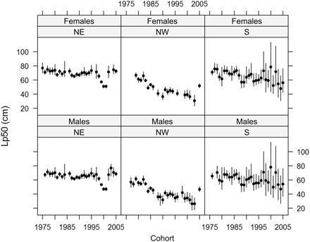
PMRN midpoints (Lp50s) for age 3 male and female North Sea cod from the NE (cohorts 1976–2005), NW (cohorts 1979–2005), and S (cohorts 1976–2005) subpopulations. The 95% credible intervals are shown as horizontal bars and incorporate error from the growth model.

Trends in potential explanatory factors

The significance of temperature to the spatial differences in maturation probability was partially confounded by the lack of overlap in ranges between the three subpopulation regions (Figure 4). There were weak but significant positive linear temperature trends in the NE and NW (t-test; p < 0.05), and a highly significant trend in the S (t-test; p < 0.0001), so tests were based on a generalized linear model fit using γ errors and an identity link function. Biomass aged 1–3 in the first quarter survey also differed among regions, although the only subpopulation with a significant declining trend with year was the NW subpopulation (t-test; p < 0.01).

Figure 4.

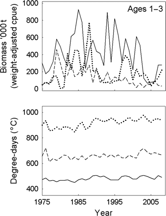
Time-trends by biomass and degree-days in summer by year by subpopulation region (stippled line, S; solid line, NW; dotted line, NE).

The life-history PMRN approach found a significant (p < 0.001) effect of sex, and sex interacting with subpopulation, age, and cohort within subpopulation. Given the significant effect of sex, subsequent analyses were conducted on males and females separately.

Linear effects of temperature and cod biomass were significant additions to the base model [Equation (10)], and were selected as the final models for both males and females (Table 3). The Lp50 values from these models are shown in Figure 5. Maturation probabilities were greater for ages 3 and 4 than for age 2. The average Lp50 was higher in the NE subpopulation, followed by NW, then S. The effect of length on maturation probability followed the same pattern. Temperature had a consistent significant positive effect in all subpopulations and sexes, except for females in the NE. Cod biomass did not have a consistent effect across population regions, but was consistent across sexes, having a positive effect in NE and a negative effect in the NW and S subpopulation. The combined effect of temperature and cod biomass can be seen in Figure 5 as additions to the cohort effect. This shows that the addition of temperature and cod biomass explains some of the decline in Lp50 values; this is due to a positive effect of temperature along with a generally increasing temperature trend experienced by the subpopulations. Figure 5 also shows that neither covariate explains the increasing positive trend in maturation probability, but that temperature increases the apparent magnitude of the trend.

Table 3.

Coefficients, standard errors, and significance (*0.05; **0.01; ***<0.001) of effects on the PMRN covariate model for cod subpopulations from the NE (p1), NW (p2), and S (p3).

	Female			Male
Parameter	Estimate	Standard error	Significance	Estimate	Standard error	Significance
Intercept	–7.28	0.6	***	–3.27	0.47	***
Length	0.08	0.01	***	0.07	0.01	***
Factor(age)3	1.20	0.16	***	0.90	0.15	***
Factor(age)4	1.23	0.35	***	0.72	0.36	*
p1	9.58	1.82	***	8.08	1.65	***
p2	2.18	1.06	*	0.80	0.67
Length:p1	0.07	0.01	***	0.12	0.01	***
Length:p2	0.04	0.01	***	0.05	0.01	***
Factor(age)3:p1	–1.65	0.33	***	–2.24	0.32	***
Factor(age)4:p1	–2.40	0.48	***	–2.73	0.48	***
Factor(age)3:p2	–0.57	0.27	*	–0.74	0.25	**
Factor(age)4:p2	–1.90	0.61	**	–0.50	0.55	–
p3:b	–0.03	0.04	–	–0.14	0.04	***
p1:b	0.38	0.07	***	0.42	0.07	***
p2:b	–0.43	0.12	***	–0.13	0.08	–
p3:t	2.17	0.33	***	0.32	0.28	–
p1:t	3.90	0.74	***	4.14	0.69	***
p2:t	0.12	0.49	–	0.39	0.38	–

Figure 5.

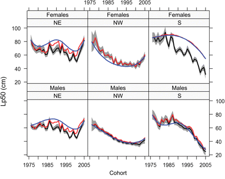
Life-history Lp50 estimates for 3-year-old cod plotted against cohort for each sex and subpopulation. The black line shows the model fit in which temperature and cod biomass were used in addition to the smooth trend in cohort; 95% pointwise credible intervals are denoted by the shaded region. The red line represents the same model, but with temperature fixed at the 1975 level to show the temperature effect, and the blue line shows the cohort effect with both temperature and conspecific biomass fixed at 1975 levels. Note that the credible intervals incorporate error from the growth model.

Discussion

Although past estimates of Lp50 values have often considered seasonal or annual temperature variation when considering the causes of shifts in maturation reaction norms (Barot et al., 2004b; Mollet et al., 2007; Pardoe et al., 2009), the life-history PMRN approach presented here provides the first method of integrating potential environment effects over the years that a cohort matures. The need for PMRN models to include temperature experienced during the maturation decision phase, rather than annual temperature, was demonstrated experimentally by Tobin and Wright (2011). The Lp50 estimates from both the demographic (Barot et al., 2004b) and the new life-history PMRN approaches were broadly consistent. The difference was greatest in the S subpopulation after 1995, with estimates from the life-history approach lying below and with smaller credible intervals than the retrospective demographic approach. There were several contributing factors to the difference in the size of credible intervals, one being that smoothing was used in the life-history approach, as opposed to treating cohort as a factor. The difference in levels is possibly due to a combination of factors. Very few immature fish were sampled at ages 3 and 4 in the S after 1999. Most age 3 and 4 fish are >35 cm and very few are <30 cm, so the data were extreme with respect to the parameters being estimated, although this is complicated by the fact that information on slopes and intercepts in both models were shared across ages and cohorts. Indeed, the approaches were modelling different things: the retrospective demographic approach assumed that the maturity ogives are linear with length on the logistic scale; this gives rise to PMRNs that tend to be non-linear on the logistic scale. The life-history approach assumed that PMRNs were linear with length on the logistic scale; this results typically in asymmetrical maturity ogives.

Declines in the values of Lp50 were evident within the North Sea cod stock, but the magnitude of decline differed among the three subpopulations examined. Although age and size close to spawning time may not be an accurate indicator of the energetic state of a fish around the time of its maturation decision (Wright, 2007), the magnitude of Lp50 changes in the NW subpopulation corresponds to more than an annual length increment. As maturation in cod is an annual decision (Davie et al., 2007) and size reflects earlier growth and condition, such marked shifts in Lp50 values reflect substantial changes in the energetic status of a fish around its maturation decision time. The magnitude and rate of Lp50 change found in the NW subpopulations is comparable with that found in Georges Bank cod stocks (Barot et al., 2004b) and stocks found off Newfoundland (Olsen et al., 2004), and close to the highest reported for cod and indeed any other fish species (Jørgensen et al., 2007). Northwest Atlantic cod stocks have declined substantially, as have the two most affected North Sea subpopulations (Holmes et al., 2008). In contrast, the small change in Lp50 found in the NE subpopulation is more in line with the low rates of change in the Northeast Arctic (Heino et al., 2002) and Icelandic cod stocks (Pardoe et al., 2009). Assuming that genetic selection is involved, a downward trend in the reaction norm is expected to stop once it falls below the size threshold at which selection no longer has any effect (Ernande et al., 2004), i.e. below the minimum size of capture that is close to the minimum landing size of 35 cm. In NW subpopulations, the Lp50 of all age groups came close to this threshold, so the trend might weaken in future.

The proportion maturing at age would be expected to differ among subpopulations even if they all had the same PMRN, because of differences in growth rate. However, this study indicates that most of the reported change in age at maturity of North Sea cod (Oosthuizen and Daan, 1974; Rijnsdorp et al., 1991; Yoneda and Wright, 2004) can be explained by the marked downward shift in PMRN midpoints from what were historically important components of the stock. Hence, the primary cause of changes in maturity at age was neither a density-dependent compensatory response nor an effect of a more favourable environment for somatic growth. In the NW population, there has also been a reduction in prespawning condition and an increase in weight-specific fecundity (Yoneda and Wright, 2004), contrary to expectations of a compensatory response (Trippel, 1995).

In the period before this study, cod throughout the North Sea matured much larger (L₅₀ > 64 cm; Holt, 1893) than currently found in the southern and northwestern North Sea. Even by the 1970s, Oosthuizen and Daan (1974) found that cod lengths at 50% maturity for the S subpopulation had decreased. At that time, there was no evidence for a regional difference in length at maturity between cod from the NW and S, with 50% maturity at around 59 cm and age 3 in the late 1960s (Oosthuizen and Daan, 1974; Yoneda and Wright, 2004). However, the present study indicates that the rate of decline in maturation probability since the 1980s was greater in the NW subpopulation. This would explain why differences in the size at maturity were found in age 2 cod from the NW and S, in a recent common environment experiment (Harrald et al., 2010). Although a large proportion of cod from the NW and S subpopulation now spawn at age 2, this is not the case in the NE. Moreover, cod in the NE still mature around a size similar to that in the 1970s and more than a century ago (see Holt, 1893). Even smaller differences in maturation reaction norms over spatial scales have been found in age 2 coastal cod inhabiting fjords along the Skagerrak coast (Olsen et al., 2008). The proximity between the Skagerrak and the late-maturing NE subpopulation region further highlights the fine scale of adaptive structuring in cod.

As applications of PMRN focus on a specific geographic region, it is important to consider whether apparent changes in Lp50 values could have arisen through colonization of early maturing genotypes from other areas (Andersen and Brander, 2009). Comparison of maturity–size relationships in areas next to the North Sea indicates that colonization is unlikely to have been important. Although some juveniles from the NE may intermix with coastal subpopulations in the Skagerrak before returning to the North Sea (Svedäng and Svenson, 2006), they mature at much greater sizes and ages (Olsen et al., 2008). Moreover, recent Lp50 values of first-maturing cod in the NW were lower than those found in cod off the Scottish west coast in the 1970s (Yoneda and Wright, 2004). This is not to say that collapse and recolonization of cod spawning areas in the North Sea cannot happen, because there is genetic evidence for this in one small region of the North Sea (Hutchinson et al., 2003). Nevertheless, tagging studies suggest that the relatively limited home ranges of the three subpopulations investigated have not changed during the period of this study (Wright et al., 2006; Righton et al., 2007). Therefore, differences in Lp50 values among subpopulations found in the present study are likely to reflect an adaptive response to local conditions rather than the confounding effect of colonization.

The rapid decline in maturation probability in the NW and S subpopulations took place following the near collapse of spawning biomass in these regions during the 1980s (Holmes et al., 2008). In the previous two decades, fishing mortality on ages 2–10 exceeded 1.0, and nearly all demersal fishing effort was concentrated in the coastal NW and southern North Sea (Jennings et al., 1999; Greenstreet et al., 2009; ICES, 2009). Conversely, until the current decade, spawning biomass remained high (Holmes et al., 2008), and fishing effort was low (Greenstreet et al., 2009) in the one region where the change in PMRN midpoints has been negligible. Catch curves derived from the first 10 years of survey data used in the present study similarly indicate a regional difference in total mortality, with Z=0.7 for ages 2–5 in the NE compared with 1.1 in the NW and S subpopulations. Consequently, it appears that mortality was historically much higher on the two subpopulations that have undergone the greatest change, so selection for early maturity would be expected to have been higher.

Summer temperature also explained some of the variation in maturation probability. Temperature can have a direct positive effect on gametogenesis during the maturation decision phase (Dhillon and Fox, 2004; Tobin and Wright, 2011), which would explain the positive effect on maturation probability found here. However, temporal trends in temperature within population regions were small or insignificant, and they did not explain the highly significant negative trends in PMRN midpoints. The regional difference in temperature range may have contributed to the difference among subpopulations, but the lack of overlap in temperature ranges confounds analysis of such an effect. The significant effect of competitive biomass was difficult to explain because it was both positive and negative, depending on subpopulation. Significant interactions in the life-history PMRN model were also not consistent among subpopulations. Modelling interactions as random effects would be an appropriate means of examining the significance of these terms more fully, and the development of such a model has started.

The different trends in maturation probability among subpopulations of North Sea cod underscores the need to account for population structuring in assessing maturation changes. Stock-level sampling may become biased towards the most abundant subpopulation as fish from areas declining in abundance become too scarce to be included in stratified sampling programmes. Consequently, if rapid declines in PMRN reflect a collapsing stock component, as found here, stock-level estimates will tend to underestimate the magnitude of change. Few other PMRN studies have tested for substock variation in maturation reaction norms. Mollet et al. (2007) found no difference in the maturation reaction norms of sole (Solea solea) between spawning areas in the German Bight and Dutch–Belgian coastal areas. Pardoe et al. (2009) attempted to consider population structure in their application of PMRN by weighting samples from different components of the Icelandic cod stock. However, weighting could still give a misleading trend if life-history responses to environmental change or selective pressures diverged between different subpopulations comprising that stock.

In conclusion, although one cannot be certain of the causes of the changes in maturation probability observed, it is possible to rule out some explanations. The slowest-growing subpopulation matured larger, contrary to expectations from counter-gradient selection (Conover et al., 2006). Further, neither regional temperature nor conspecific biomass could fully account for the highly significant negative trends in Lp50 values. Therefore, given the likely intense periods of size-selection mortality in the NW and S subpopulations, selection for early maturing genotypes appears to be the most parsimonious explanation for the temporal changes in maturation probability. Recent debate on fisheries-induced evolution has focused on the apparent rate of evolution estimated from PMRN studies and the lower rates expected from the estimation of selection differentials (Andersen and Brander, 2009). The results of the present study indicate that the combined effects of phenotypic response to temperature and genetic selection for earlier and smaller size at maturation could be additive, leading to bias in the estimate of evolutionary rates based on PMRN alone. Given that warming trends are evident in many of the regions where changes in fish maturation schedules have been reported, there is a need to revisit the potential contribution of temperature on the apparent rate of evolution inferred from the demographic PMRN approach.

Acknowledgements

This study was carried out with financial support from the European Commission, as part of the Specific Targeted Research Project Fisheries-induced Evolution (FinE, contract number SSP-2006-044276) under the Scientific Support to Policies cross-cutting activities of the European Community's Sixth Framework Programme. It does not necessarily reflect the views of the European Commission, and does not anticipate the Commission's future policy in the area. The work was also supported by Scottish Government ROAME MF 0764. We also acknowledge the contribution of the ICES IBTS survey and staff on the FRV “Clupea” and FVs “Auriga”, “Charisma”, “Falcon”, “Genesis”, “Helenus”, “Jasper”, “Sunbeam”, “Tranquility”, “Veracious”, and “Zenith” for samples. Rob Fryer provided helpful comments on the statistical analysis and manuscript.