Utility of 18-kHz acoustic data for abundance estimation of Atlantic herring (Clupea harengus)

Abstract

Saunders, R. A., O'Donnell, C., Korneliussen, R. J., Fässler, S. M. M., Clarke, M. W., Egan, A, and Reid, D. 2012. Utility of 18-kHz acoustic data for abundance estimation of Atlantic herring (Clupea harengus) – ICES Journal of Marine Science, 69: 1086–1098.

Current acoustic survey protocols for Atlantic herring (Clupea harengus) abundance estimation are principally dependent upon 38-kHz backscatter data. This can constitute a substantial problem for robust stock assessment when 38-kHz data are compromised. Research vessels now typically collect multifrequency data during acoustic surveys, which could be used to remediate such situations. Here, we investigate the utility of using 18- and 120-kHz data for herring abundance estimation when the standard 38-kHz approach is not possible. Estimates of herring abundance/biomass in the Celtic Sea (2007–2010) were calculated at 18, 38, and 120 kHz using the standard 38-kHz target-strength (TS) model and geometrically equivalent TS models at 18 and 120 kHz. These estimates were compared to assess the level of coherence between the three frequencies, and 18-kHz-derived estimates were subsequently input into standard 38-kHz-based population models to evaluate the impact on the assessment. Results showed that estimates of herring abundance/biomass from 18 and 38 kHz acoustic integration varied by only 0.3–5.4%, and acoustically derived numbers-at-age estimates were not significantly (p > 0.05) different from 1:1. Estimates at 120 kHz were also robust. Furthermore, 18-kHz-derived estimates did not significantly change the assessment model output, indicating that 18-kHz data can be used for herring stock assessment purposes.

Introduction

Acoustic survey techniques are used widely to provide data on fish abundance and distribution (Simmonds and MacLennan, 2005). Such techniques are particularly well suited to pelagic fish, such as Atlantic herring (Clupea harengus), which form distinct schools in midwater that can be detected effectively by echosounders. The general approach is that echo intensities of acoustically insonified fish schools are integrated and converted into fish numbers (or density) using species-specific target-strength (TS) relationships. TS relationships quantify the sound backscattering potential of a target species, which is largely dependent on acoustic frequency, body size, presence/absence of a swimbladder, and target orientation (McClatchie et al., 1996; Horne and Jech, 1999). Acoustic estimates of abundance are, therefore, highly dependent on accurate measurements of TS (Demer and Conti, 2005). Acoustic surveys are an effective tool for monitoring commercially targeted fish stocks because they enable almost continuous detection of fish throughout the water column at high resolution (typically one sample s⁻¹ by 20 cm in the vertical with 1 ms pulse duration at 38 kHz) over a relatively broad spatial scale. Acoustically derived estimates of herring abundance are now an integral component of routine stock assessments that are usually treated as indices to tune population assessment models (Simmonds, 2003).

ICES has adopted standard protocols for acoustic herring surveys and for calculating acoustic estimates of abundance for stock assessment purposes (ICES, 1982, 2008). The currently adopted approach is to calculate herring abundance from acoustic data collected at 38 kHz using a simple TS relationship of the form TS = 20log₁₀(L) – b₂₀, where L is fish length and b₂₀ is a species-specific intercept value at this acoustic frequency (Simmonds and MacLennan, 2005). ICES recommendation for North Sea herring is a TS–L relationship of TS = 20log₁₀(L) – 71.2, following Edwards and Armstrong (1981) and Nakken and Olsen (1977). However, research vessels often collect acoustic data at several acoustic frequencies (typically 18, 38, 120, and 200 kHz) during fishery surveys that could, in theory, also be used to provide herring abundance estimates. Optimal acoustic frequencies for measuring fish schools are those that are not affected by noise over the depth range occupied by the target species, and where the wavelength is similar to, or smaller than, the target size (Horne and Clay, 1998). Between 90 and 95% of the acoustic backscatter from fish possessing gas-filled swimbladders is from these organs (Foote, 1980). In the case of most schooling fish species, 38 kHz is an appropriate compromise between range and resolution, and most fishery survey and abundance estimation protocols have, therefore, become highly dependent on 38-kHz data. However, 18 kHz is also a suitable frequency for many commercially targeted fish species (Simmonds and MacLennan, 2005), and 18-kHz data could theoretically be used for herring abundance estimation and subsequent assessment purposes, assuming that an appropriate TS–L relationship is used to scale the acoustic backscatter. The frequency could also be potentially better than 38 kHz in some situations, as it has a greater noise-free range, and the species is a more suitable point target at 18 kHz (Simmonds and MacLennan, 2005). Data analysis and echogram scrutinizing procedures would have to consider, though, that some targets, such as siphonophores, Mullers pearlside (Maurolicus muelleri), or other small fish/fish larvae (myctophids) may be very strong acoustic scatterers at 18 kHz, but weak at other frequencies (Fernandes et al., 2006). Several small mesopelagic fish species also have a variable scattering response at 18 kHz that is largely associated with diel vertical migration (DVM) behaviour and swimbladder resonance, and these animals are often stronger acoustic scatterers at night and periods of DVM than during the day (Godø et al., 2009). Thus, echoes from such species could be mistaken for herring in scenarios where there are too few trawl samples to ground-truth the acoustic observations adequately, particularly when surveys are conducted at night and in more off-shelf regions. A further consideration is that the acoustic beam angle at 18 kHz is wider than that at 38 kHz (∼11° vs. 7°; Table 1), so it is possible that more fish could be insonified at 18 kHz in some situations. For example, if there is systematic horizontal avoidance athwartship, the wider beam might measure more fish than a narrower beam. If the horizontal avoidance was enough to cause fish to leave the beam of the 38-kHz sounder, but not the wider beam of the 18-kHz sounder, the fish density may also appear higher. However, there is evidence that fish avoidance might not be a significant source of bias on research surveys (Fernandes et al., 2000), and the mismatch in acoustic beam widths may be minimized by restricting multifrequency comparisons to certain sampling depths. The additional effective sampling volume at 18 kHz with an 11° beam angle, for example, is ∼260 m³ at 100 m range and 6591 m³ at 500 m range compared with that at 38 kHz with a 7° beam angle (Ona and Mitson, 1996).

Table 1.

Transducer specifications and settings during acoustic data collection in 2010.

	Frequency (kHz)
Specification	18	38	120	200
Transducer type	ES18-11	ES38B	ES120-7	ES200-7
Transducer depth (m)	8.8	8.8	8.8	8.8
Maximum power (W)	2 000	2 000	500	300
Pulse duration (ms)	1.024	1.024	1.024	1.024
Sample length (m)	0.194	0.194	0.194	0.194
Ping interval (s)	1.0	1.0	1.0	1.0
Bandwidth (kHz)	1.19	2.43	8.71	10.64
Sv transducer gain (dB)	23.02 (±0.08)	25.85 (±0.09)	25.49 (±0.21)	25.69 (±0.47)
Two-way equivalent beam angle (dB)	–17.0	–20.6	–20.8	–20.7
3-dB beam width alongship (deg)	10.47	6.93	7.21	6.74
3-dB beam width athwartship (°)	10.67	6.96	7.26	6.75
Absorption coefficient (dB km−1)	2.51 (±0.17)	9.55 (±0.44)	42.79 (±2.75)	62.2 (±5.60)
Sound velocity (m s−1)	1501.3 (±4.2)	1501.3 (±4.2)	1501.3 (±4.2)	1501.3 (±4.2)
Sa correction	–0.57 (±0.23)	–0.64 (±0.20)	–0.71 (±0.31)	–0.46 (±0.17)

The observed ranges of the parameters that varied between surveys are given in parentheses.

Although modern scientific echosounders are becoming increasingly robust, there can be instances when they fail, leading to a loss of data at a particular frequency during a survey. For example, physical failure in one of the system's transducer cables can be a problem with scientific echosounders that are mounted on retractable drop keels, as is the case with RV ‘Celtic Explorer’, where changes in tension on transducer cables can cause circuit damage over time, which will lead to the loss of one or more quadrants on a split-beam transducer. This causes distortions in the acoustic beam pattern on either transmit or receive, or both. Any data collected subsequently may still appear to be superficially normal, but the integrated values will be incorrect. In situations where acoustic abundance indices are solely based on one acoustic frequency, as is the case with the current ICES herring assessment protocols (exclusively 38 kHz), there can be serious implications for the assessment and management advice when data at this frequency are compromised. The availability of data at other suitable acoustic frequencies, such as 18 kHz, collected simultaneously during a survey could, therefore, be very useful in such scenarios, if protocols for the use of these data were available. However, there have been few published studies on the use of 18-kHz-derived herring abundance estimates for management purposes, and there is currently little guidance from ICES documentation on how 18-kHz data might be used to estimate herring abundance when 38-kHz data are unavailable.

The Irish Marine Institute has conducted an annual acoustic survey for herring in the Celtic Sea (ICES Divisions VIIaS, VIIj, and VIIg) onboard RV ‘Celtic Explorer’ for stock assessment purposes since 2004. In 2010, problems with the 38-kHz transducer cable resulted in quadrant dropout and compromising of the acoustic data collected. As the current ICES herring assessments are conducted with this index of abundance, this loss of data constituted a significant obstacle for the 2010 Celtic Sea herring assessment. In this paper, we investigate an alternative approach for calculating herring abundance using fully calibrated 18-kHz data. We also compare abundance estimates at 18, 38, and 120 kHz for previous acoustic surveys in the Celtic Sea and evaluate how useful 18-kHz-derived estimates are for stock assessment purposes in context with the standard 38-kHz herring assessment time-series.

Material and methods

Data collection

Acoustic data were collected onboard RV ‘Celtic Explorer’ during the Celtic Sea Herring Acoustic Survey in October 2007–2010 (Figure 1). Each year, the survey timing was standardized at around 6–26 October to minimize temporal aliasing. Data were collected using a Simrad EK60 scientific echosounder operating four transducers at frequencies of 18, 38, 120, and 200 kHz. The transducers were mounted adjacently (within 0.3 m) on a drop keel and were deployed ∼3 m below the hull. Echosounder properties and typical settings used during the surveys are shown in Table 1. The echosounder was calibrated using standard reference targets (64- and 60-mm copper spheres for 18 and 38 kHz, respectively, and a 38.1-mm tungsten carbide sphere for both 120 and 200 kHz) following the method of Foote et al. (1987). Data were collected during both day and night on these surveys, and the maximum bottom depth was ∼112 m in the survey area.

Figure 1.

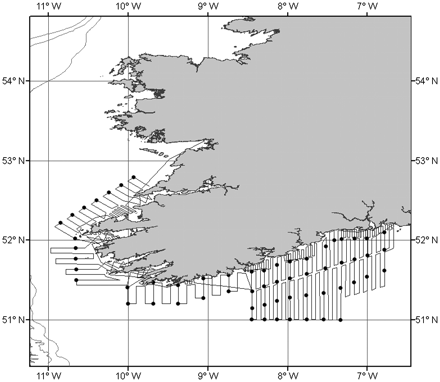
The Celtic Sea Herring Acoustic Survey study region. Filled circles show positions of hydrographic stations, and the 200-, 300-, and 500-m depth contours are also shown. Transect spacing ranges from 1 to 4 nautical miles.

During the surveys, major echotraces were sampled with a pelagic trawlnet with an effective sampling aperture of ∼330 m² and graded-mesh sizes reaching a minimum of 0.2 m at the codend. Each net haul was towed for ∼45 min at a speed of 3–4 knots. Net sampling depths were monitored using Scanmar depth sensors and a netsounder (50 kHz) fitted to the net headline. Trawl data provided information on echotrace species and size composition, as well as information on herring age and maturity status. A total of 120 trawl hauls were conducted over the four surveys (typically 30 hauls per survey), of which 35 hauls were composed exclusively of herring and 67 hauls were composed of >50% herring.

Acoustic data analysis

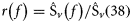
Acoustic data were analysed using Myriax Echoview software. Echograms were first scrutinized for regions of bad data (e.g. times off transect, periods of interference, and near-surface dead zones), and seabed echoes were masked such that all echograms were standardized for comparison. The near-surface dead zone was defined at 15 m depth to alleviate potential problems with surface bubble layers during bad weather, and the seabed exclusion zone was defined as 2 m above the 18-kHz bottom detection line. There was no evidence of herring shallower than 15 m during the four surveys. Echotraces from herring targets were then identified using information from the net hauls (Reid et al., 2000). All echograms were synchronized and scrutinized so that nautical-area backscattering coefficient (NASC; s_A) data from exactly the same herring echotraces could be exported at each frequency for the analysis (Figure 2). Due to potential issues with complex high-frequency backscattering (Holliday and Pieper, 1995), the analysis focused on 18-, 38-, and 120-kHz data, and the 200-kHz data were retained for further analysis. Figure 3a and b compared with c shows that the frequency-response r(200 kHz) for herring, i.e. the backscatter at 200 kHz relative to 38 kHz, is more uncertain than r(18 kHz) and r(120 kHz).

Figure 2.

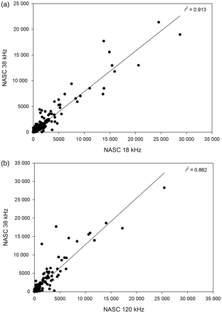
Relationship between herring backscatter (NASC) at (a) 18 and 38 kHz and (b) 120 and 38 kHz during the Celtic Sea Herring Surveys in 2009, 2008, and 2007. The solid line is the regression line.

Figure 3.

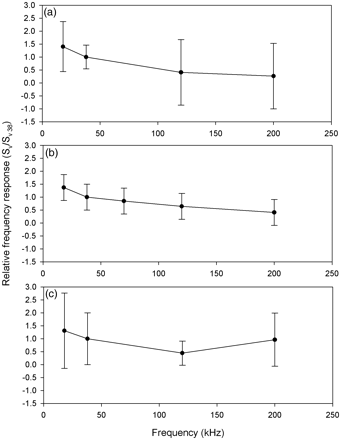
Mean values of relative frequency response r(f) for Atlantic herring schools (a) around Ireland between 2007 and 2009, (b) in the Norwegian Sea (1996–2010), and (c) in the North Sea (Fässler et al., 2007). The error bars represent the 95% confidence intervals.

Estimates of herring abundance and biomass at 38 kHz (for 2007–2009) were calculated using ICES standard protocols (ICES, 1982, 2008) following the long-established model of Dalen and Nakken (1983) and MacLennan (1990):

(1)

where subscript i refers to length groups at 0.5-cm intervals, ρ_a,i is the area fish density (number nautical mile⁻²), s_A,i is the mean NASC estimated from the actual length distribution (Dalen and Nakken, 1983), and [σ_bs,i] is the average backscattering cross-section per fish. If L_i is the mean length of group i in cm, [σ_bs,i] in m² is derived from the recommended length-based, TS function (ICES, 2008):

(2)

The number of herring within the j^th geographical region (e.g. 1° × 0.5° rectangle) is the sum of the ρ_a,i over all length groups (i = 1 to n) multiplied by the region area in nautical mile². Summing the results over all regions (j = 1 to m) yields the total number of herring (N_F) within the surveyed area:

(3)

Estimates of herring biomass (in 1000 t) were calculated from numerical abundance using the recommended allometeric length–weight relationship to scale the observed herring length frequency distributions (ICES, 2008):

(4)

where L is length in cm.

In addition, acoustic estimates of spawning-stock biomass (SSB), spawning-stock number (SSN), and abundance by age class (0–9 winter ring counts) were also calculated using data obtained from the trawl haul samples according to standard protocols (ICES, 2008). In this procedure, acoustic backscatter attributed to herring was partitioned into these age groups according to the actual proportions of the cohorts observed in the corresponding net trawls. SSB and SSN were calculated using a maturity ogive (derived from trawl data) applied to the abundance-at-age data. Data from the closest net trawls were used to scale herring backscatter in regions where no net sampling was possible, and spatially contiguous (usually within 5 nautical miles) trawl data were combined in regions where <100 individuals were sampled.

18- and 120-kHz herring TS

Estimates of abundance, SSB, and biomass were calculated at 18 kHz for all 4 years following the same procedure as above. As there are no recommended TS–L relationships at this frequency, we devised a simple TS model as follows. First, we assumed herring backscatter at both 18 and 38 kHz to be in the geometric scattering region, where backscatter is proportional to the cross-sectional area of the insonified object. Consequently, the TS at these two frequencies can be derived using the common TS = 20log₁₀(L) – b₂₀ relationship (Demer and Martin, 1995; Fernandes et al., 2006). Given this same geometric dependency at the two frequencies, it should then be possible to offset the intercept value of the standard 38-kHz TS model according to the difference in frequency response of herring at 18 kHz. Secondly, the frequency-specific characteristics of 200 confirmed herring echotraces detected over three surveys (2007–2009) were compared using the frequency-response measure r(f) (Korneliussen and Ona, 2003):

(5)

where ŝ_v(f) is the mean volume backscattering coefficient of the echotrace at frequency (f). Our analyses revealed that herring backscatter was ∼40% stronger at 18 than at 38 kHz [mean r(f) = 1.4 ΔdB relative to 38 kHz; Figure 3a]. This was supported strongly by ground-truthed acoustic data obtained from five herring surveys conducted in the Norwegian Sea (September–December 1996, 1999, 2005, 2009, and 2010) by the Institute of Marine Research (IMR) (Figure 3b), and by published data from multifrequency studies on Atlantic herring in the North Sea (Figure 3c; Fässler et al., 2007). Finally, we calculated our 18-kHz herring TS model based on this observed frequency response [r(f) = 1.4 ΔdB; which is 1.46 in 10log form, i.e. 10 × log(1.4) = 1.46] as:

(6)

and

(7)

where L is length in cm.

Herring abundance and biomass indices at 120 kHz were calculated using the same standard procedures as adopted for 38 kHz. The 120-kHz TS model was also determined using the same approach as that described above for 18 kHz. Our analyses, together with data from the Norwegian Sea and the North Sea, indicated that the mean r(f) of herring at 120 kHz was 0.5 ΔdB (–2.98 in 10log form) relative to 38 kHz (Figure 3). Therefore, the 120-kHz TS model was calculated as:

(8)

and

(9)

where L is length in cm.

Impact on analytical stock assessment and short-term forecast

In order to evaluate the impact of the use of the abundance data derived from the 18-kHz sounder, the data were used as part of the survey tuning index in the standard stock assessment method used for this stock (Annex 5 in ICES, 2010). This was carried out using Integrated Catch at Age Analysis (Patterson and Melvin, 1996). The analysis compared the standard operating procedure using the time-series of 2002–2009 survey estimates based on 38-kHz data with a time-series where the years 2007–2009 were replaced with estimates derived from 18-kHz data. It was not possible to extend this analysis to 2010, owing to the lack of 38-kHz data for that year. A short-term stock deterministic forecast was also calculated using the Multi Fleet Deterministic Projection (MFDP) model (Smith, 2000) with data from each of the assessment runs. This was conducted to evaluate the impact of the assessment using the 18-kHz abundance time-series on the scientific advice, mimicking the advisory process of setting total allowable catch (TAC) options.

Results

The overall herring biomass, SSB, SSN, and abundance in the Celtic Sea calculated from the 18-kHz data were substantially higher in 2010 than in 2007, 2008, and 2009, and these estimates constitute the highest in the region to date [153 769 t, coefficient of variation (CV) 19.4%; 121 719 t, CV 20.5%; 1064 million individuals, CV 19.2%; and 1415 million individuals, CV 19.2%, respectively; Table 2]. Although the 18-kHz-derived estimates are intrinsically valid, the acoustic herring stock abundance time-series is predominantly based on 38-kHz estimates. Therefore, we compared estimates at 18 and 38 kHz from surveys conducted in 2007, 2008, and 2009 to set the values in context and determine if the 18-kHz-derived estimates for 2010 could be used for the otherwise 38-kHz-based assessment models (Table 2). In 2009, the overall herring biomass estimates at 18 and 38 kHz varied by <1%, and the SSB, SSN, and abundance values varied by ∼2% between the two frequencies. The level of variation between the two acoustic frequencies was also relatively low for the 2008 survey, the difference being ∼1–3% for the biomass SSN and SSB estimates. The largest difference was 4.3% for the abundance estimates in 2008. The level of variation was also relatively low for the 2007 comparisons (<2% for biomass, SSN, and SSB estimates, and ∼5% for numerical abundance).

Table 2.

Acoustic estimates of herring abundance in the Celtic Sea at 18 and 38 kHz, October 2010–2007.

	18 kHz (CV%)	38 kHz (CV%)	120 kHz (CV%)	% difference 18 and 38 kHz	% difference 120 and 38 kHz	% difference 18 and 120 kHz
2010
Biomass	153.8 (19.4)	– (–)	161.2 (18.5)	–	–	4.8
SSB	121.7 (20.5)	– (–)	128.3 (18.6)	–	–	5.4
Abundance	1414.7 (19.2)	– (–)	1476.8 (18.3)	–	–	4.4
SSN	1064.0 (19.2)	– (–)	1123.0 (18.3)	–	–	5.5
2009
Biomass	119.5 (23.7)	119.1 (22.7)	123.8 (25.4)	0.3	3.8	3.6
SSB	93.0 (24.6)	90.9 (24.0)	94.0 (25.7)	2.3	3.3	1.1
Abundance	1122.4 (23.5)	1147.4 (23.1)	1213.5 (25.4)	2.2	5.4	8.1
SSN	541.2 (19.2)	526.6 (23.1)	544.5 (25.4)	2.7	3.3	0.6
2008
Biomass	94.8 (22.7)	93.3 (19.6)	97.1 (22.2)	1.6	3.9	2.4
SSB	93.4 (23.0)	90.9 (20.0)	95.3 (22.6)	2.7	4.6	2.0
Abundance	735.0 (22.3)	768.6 (19.2)	761.7 (22.1)	4.3	0.9	3.6
SSN	622.3 (22.3)	606.0 (19.2)	631.4 (22.1)	2.6	4.0	1.4
2007
Biomass	54.2 (19.9)	53.2 (23.0)	57.1 (23.3)	1.9	6.8	5.3
SSB	45.6 (21.7)	46.4 (24.9)	49.0 (24.9)	1.7	5.3	7.5
Abundance	478.8 (18.8)	454.0 (21.6)	497.1 (22.6)	5.3	8.6	3.8
SSN	341.3 (18.8)	347.5 (21.6)	368.5 (22.6)	1.8	5.6	7.9

Biomass and SSB estimates are in units of 1000 t, and abundance and SSN estimates are millions of individual fish.

The results of the 38- and 120-kHz comparisons also showed that the estimates of abundance and biomass were very similar between the two frequencies (Table 2). In each year, the 120-kHz indexes of biomass, SSB, abundance, and SSN were slightly higher than those derived from 38-kHz data, but the overall level of variation was only in the order of 3.3–5.4% in 2009, 0.9–4.6% in 2008, and 5.3–8.6% in 2007. The results further showed that the 120-kHz estimates were also comparable with those derived from 18-kHz data in each year, the level of variation generally being ∼1–8% greater than that at 18 kHz (Table 2).

Acoustically derived numbers-at-age estimates for adult herring (ages 2 and older) are used as tuning indices in the herring assessment models and are important for estimating the population structure of the Celtic Sea herring stock. Thus, the overall assessment model output and resulting management advice could be impacted if there were differences in the acoustic estimates of herring year-class abundance between different acoustic frequencies. Our analyses revealed that there were no significant differences in the acoustically derived numbers-at-age estimates (ages 0–9) at 18 and 38 kHz (p > 0.05; Students t-test) for any of the three surveys, and the estimates did not deviate significantly (p > 0.05; paired two-sample t-test) from 1:1 (Figure 4a). A similar trend was also obtained for the 38- and 120-kHz numbers-at-age comparison (Figure 4b), and there was no statistically significant difference between the estimates at these two frequencies (p > 0.05). Inspection of the abundance estimates by age class revealed that the main differences between the total abundance estimates at 38 and 18 kHz in 2007 and 2008 were due to slight differences in a single year class, either the 0-ring or the 1-ring group (Table 3). In 2008, the abundance of the 0-ring group was slightly lower at 18 than at 38 kHz (54.7 compared with 98.7 million individuals), and in 2007, the abundance of the 1-ring group was slightly higher at 18 kHz (137.0 compared with 106.0 million individuals). There were also slight differences in both of these two age groups in 2009, with the estimates ∼20 million individuals higher in magnitude at 38 than at 18 kHz (Table 3). The numbers-at-age estimates were considerably less variable between the two acoustic frequencies for the 2–9-ring age groups in each year, which resulted in relatively stable SSN estimates between 18 and 38 kHz. The pattern in variation between the 120- and 38-kHz numbers-at-age estimates was similar to that observed for the 18- and 38-kHz comparison in each year in that the main differences generally occurred within a single age class in the juvenile component in the population (either the 0-ring or the 1-ring age class), whilst the adult component (2–9-ring classes) was less variable. However, the 18-kHz-derived numbers-at-age estimates matched those derived from the 38-kHz data more closely than the 120-kHz-based estimates, suggesting that 18-kHz data were more suitable for the overall herring assessment. Thus, the 18-kHz estimates were used in the assessment model comparisons, and the 120-kHz data were retained for further analysis.

Figure 4.

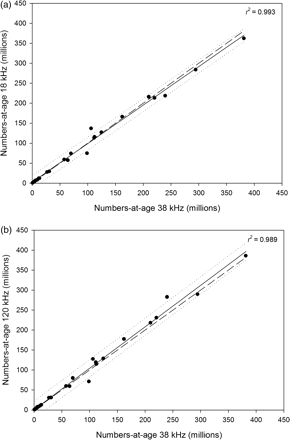
Comparison of the numbers-at-age estimates at (a) 38 and 18 kHz and (b) 38 and 120 kHz in the Celtic Sea during 2009, 2008, and 2007. The solid line is the regression fit and the heavy dashed line is the 1:1. The small dashed lines are the 95% confidence limits of the regression fit. Estimates did not deviate significantly from 1:1 (p > 0.05; paired two-sample t-test).

Table 3.

Acoustic estimates of herring abundance (millions of individuals) by age class (winter rings) in the Celtic Sea between 2010 and 2007.

	2010			2009			2008			2007
Age	18 kHz	38 kHz	120 kHz	18 kHz	38 kHz	120 kHz	18 kHz	38 kHz	120 kHz	18 kHz	38 kHz	120 kHz
0	4.7	–	4.0	218.7	239.5	282.8	54.7	98.7	71.1	0.6	0.5	1.0
1	346.2	–	349.7	362.4	381.4	386.1	58.0	64.0	59.2	137.0	106.0	127.6
2	548.9	–	582.3	115.9	112.0	114.8	290.6	294.5	289.9	74.3	69.8	79.9
3	155.9	–	165.3	216.0	209.8	218.2	117.1	111.4	119.4	213.1	220.3	231.0
4	193.0	–	203.7	59.0	57.5	60.1	172.8	162.0	177.6	29.3	30.6	31.0
5	65.2	–	67.9	127.3	124.6	128.7	28.9	26.7	30.5	8.4	9.0	9.0
6	91.0	–	93.9	12.0	11.7	11.7	7.1	6.2	7.7	12.1	13.1	13.0
7	6.7	–	7.0	3.5	3.7	3.7	5.8	5.0	6.3	3.3	3.7	3.5
8	3.1	–	2.9	6.4	6.3	6.5	–	–	–	0.9	1.0	1.1
9	–	–	–	1.0	0.9	0.8	–	–	–	–	–	–
Total	1414.7	–	1476.8	1122.4	1147.4	1213.5	735.0	768.6	761.7	478.9	454.0	497.1

Modelled recruitment, SSB, and mean fishing mortality (1958–2009) using abundance data from 18-kHz data for 2010 and a combination of 18- and 38-kHz data (for years 2007–2009) as input are presented in Figure 5. Results of comparative stock assessment runs showed that the stock size estimate for 2009 and the trajectories of SSB and recruitment over time displayed few differences (Figures 5a and b). The modelled fishing mortality (F) was also similar (Figure 5c). Thus, the population abundance estimation procedure for this stock was robust to the substitution of 18-kHz-based abundance estimates. Furthermore, there were only slight differences (∼2%) in the forecasted catch options that were calculated using abundance estimates at 38 and 18 kHz, indicating that the use of 18-kHz data would not have much impact on the overall management advice (Table 4).

Figure 5.

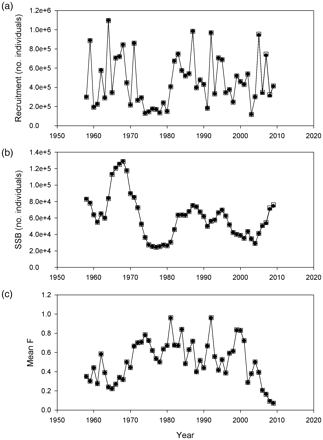
Output from the standard herring assessment models using 38-kHz (filled circles) and 18-kHz (open squares) data. (a) Estimated recruitment, (b) estimated spawning-stock biomass (SSB), and (c) mean fishing mortality (ages 2–5).

Table 4.

Standard ICES stock summaries and forecasts for Celtic Sea herring calculated using 38- and 18-kHz-derived estimates of abundance as input in the standard herring assessment model.

Rationale	Catch 2011	SSB 2011a	Basis	F 2011	SSB 2012	% TAC changeb
38-kHz data
MSY framework	16.8	72	Fmsy median estimate	0.25	67	66
F rebuilding plan	13.2	74	Fmgt	0.19	72	30
Policy paper	12.7	74	Category 1	0.18	73	25
Zero catch	0	81	F = 0	0	91	–100
	8.6	76.4	Fsq × 0.71	0.12	78.8	–15
Status quo	10.1	75.6	Fsq × 0.82	0.14	76.7	0
	11.6	74.7	Fsq × 0.98	0.165	74.6	15
	12	74.5	F2010	0.17	74	19
18-kHz data
MSY framework	17.2	72	Fmsy median estimate	0.25	68	69
F rebuilding plan	13.4	74	Fmgt	0.19	73	32
Policy paper	12.7	75	Category 1	0.18	74	25
Zero catch	0	82	F = 0	0	92	100
	8.6	77	Fsq × 0.69	0.11	80	–15
Status quo	10.1	76	Fsq × 0.82	0.14	77	0
	11.6	75.9	Fsq × 0.96	0.162	75.7	15
	12	75	F2010	0.17	75	20

Weights are in 1000 t.

^aFor this autumn spawning stock, the SSB is determined at spawning time and is influenced by fishery between 1 April and spawning.

^bCatch (assumed same as landings) in 2011 relative to TAC in 2010.

Discussion

Our results indicate that the acoustic estimates of herring abundance at 18 kHz were compatible with those at 38 kHz for the 2009, 2008, and 2007 surveys. The overall values varied by only a relatively small margin (<1–5.4%), and the use of 18-kHz-derived estimates of abundance did not have much impact on the overall assessment models. This suggests a relatively high degree of confidence in the 18-kHz estimates for the 2010 assessment, and it appears that the 18-kHz approach presented here is a suitable alternative when 38-kHz data are unavailable. Our results further indicate that the current herring assessment and management frameworks are robust enough to accommodate acoustic abundance estimates at 18 kHz. The substitution of three annual 18-kHz-derived abundance estimates into the standard 38-kHz-based acoustic time-series did not lead to significant changes in stock perception. This is because the 38-kHz-derived portion of the time-series is still the more influential component in the assessment model. It is possible that an entire time-series based on 18-kHz estimates could lead to different perceptions in herring stock, and analyses are ongoing. However, the approach presented here is not to substitute a whole time-series and does not advocate a switch to 18-kHz-based methodology, although there are several advantages to using 18 kHz instead of 38 kHz in some applications. For example, 18 kHz is less sensitive to changes in fish orientation than 38 kHz and other higher frequencies, because herring is closer to being a point-scatter at this frequency, so there is potentially less variability in the pattern of sound reflection with target orientation and angle (Godø et al., 2009). Hence, possible issues with ship motion or fish behaviour are reduced at 18 kHz. Using 18 kHz also reduces the inclusion of organisms without gas-filled organs in the acoustic analysis, as these organisms do not resonate well at 18 kHz (Holliday and Pieper, 1995), and the frequency can offer greater sampling potential for certain species at depth. In this paper, we maintain that there are advantages to adhering to a single acoustic frequency in fishery assessment applications, such as maintaining continuity with a historical time-series and reducing potential sources of unknown error. However, data collected at alternative frequencies are also highly informative, and there is much merit in adopting a more multifrequency approach during routine fish stock assessments.

A closer inspection of the survey results revealed that there were slight (but not statistically significant) differences between the 18- and 38-kHz abundance estimates (∼4–5%) that probably occurred due to slight mismatches within the 0- and 1-ring groups. During all four surveys, these smaller juvenile age groups were distributed predominantly in the more southerly sectors and occurred exclusively within mixed-school assemblages. The herring were mostly mixed with either Atlantic mackerel (Scomber scombrus) or sprat (Sprattus sprattus) of a similar body size. In the analysis, acoustic backscatter from mixed-school echotraces is allocated to species based on the proportions observed in the concurrent trawl hauls (ICES, 1982), but there could be some misallocation issues inherent in this procedure. For instance, the ability of the sample net to catch and retain fish may be different between species. It is therefore possible that backscatter from other components of the mixed schools contributed to the slight mismatch in abundance within these year classes during the 2009 and 2008 surveys. The frequency response of mackerel is different at 18 kHz compared with 38 kHz (Korneliussen, 2010), while sprat, a clupeoid fish closely related to herring, would be expected to have a frequency response closer to that of herring. Thus, the abundance estimates calculated at 18 kHz would be expected to be lower than those at 38 kHz, as is the case in 2009 and 2008, because mackerel has a lower frequency response at 18 kHz. However, species misallocation within mixed-school assemblages does not account for all of the observed variation between frequencies in this study, as the juvenile component (1-ring group) was more abundant at 18 kHz than at 38 kHz in 2007, and hence the total abundance was slightly higher.

One possible explanation for the slight discrepancy in the 2007 results could be that there is a depth-dependent difference between backscatter measurements at 18 and 38 kHz due to differences in sampling volume as a result of the different acoustic beam widths (i.e. 18 kHz may measure more samples because it has a greater beam angle than 38 kHz). However, the difference in sampling volume between the two frequencies was relatively small in this study as the maximum depth in the survey region was only ∼112 m, which would give a maximum of ∼327 m³ additional sampling volume at 18 kHz over this range. To a large extent, the results from the 120-kHz analysis also suggested that differences in sampling volume were not an issue in this particular case. The 120-kHz transducer has the same beam angle as the 38-kHz transducer (7°), and the results from these two frequencies were both highly comparable with each other and with the estimates calculated at 18 kHz. Had differences in sampling volume been an issue in this study, it would be expected that the 18-kHz-based estimates would have been consistently larger than both the 38- and 120-kHz-based estimates. However, this was not the case. Our results suggest that discrepancies in sampling volume due to small differences in beam angles might not be a major source of bias in pelagic fishery survey applications, at least at shallower depth ranges. This could be because acoustic integration measurements are expressed as a mean over the whole sampling volume (Central Limit Theorem; Urick, 1983). So, although a wider acoustic beam might measure more samples than a narrower beam, the backscatter measurements would be comparable because they are expressed as a mean over the total sampling volume.

Another possible explanation for the slight differences in abundance estimates at 18 and 38 kHz is that changes in fish physiology in response to pressure may cause differences in TS between frequencies. Depth and, hence, pressure are two factors that can affect fish TS and frequency response (Fässler and Gorska, 2009), so frequency-specific differences in backscatter measurements might occur through marked variations in fish vertical distribution (Godø et al., 2009). However, a recent modelling study of variations in herring TS over pressure/depth at various acoustic frequencies revealed that herring TS at 18, 38, and 120 kHz remained relatively constant over the ambient pressure range 1–7 bar (S. M. M. Fässler, pers. comm.; Figure 6). Therefore, marked variations in herring backscatter measurements due to depth-dependent changes in TS appear to be an unlikely source of bias over the depth range in the Celtic Sea. Other studies have also demonstrated that the frequency response of herring is relatively stable over depth (0–200 m) for these acoustic frequencies (Ona and Korneliussen, 2000), further suggesting that the changes in vertical depth distribution would not have impacted the results of this study. Furthermore, there was no evidence of pronounced variations in herring depth distribution during the four surveys, regardless of maturity status or age class, and the vast majority of schools were distributed in deeper regions of the water column, or in proximity to the seabed. All net hauls targeted at major herring echotraces were below 50 m, and the mean depth of the mixed-assemblage schools that contained juvenile herring during the 2007 survey was ∼90 m (SD 12.65), as determined using the Echoview School Detection Module (Barange, 1994; Coetzee, 2000). Thus, the slight differences observed in the 18- and 38-kHz abundance estimates are also unlikely to be attributable to differences in sampling in the surface layers.

Figure 6.

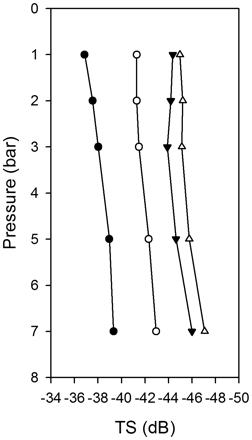
Modelled TS at four different frequencies (18 kHz, filled circles; 38 kHz, open circles; 120 kHz, filled triangles; 200 kHz, open triangles) of a 250-mm herring exposed to various water pressures ranging from 1 to 7 bar (Fässler et al., 2009). Acoustic backscatter was calculated using the Kirchoff-ray mode approximation (KRM) (Clay and Horne, 1994). TS values were averaged by fish orientation, assuming a normal tilt angle distribution with a mean of 86.9° and an SD of 14.2° (Ona, 2001).

Although the reasons for the slight mismatch between the 18- and 38-kHz abundance indices are not clear from the data, our results suggest that the main sources of error are largely confined to the 0–1-ring age-classes and not the adult component of the population (2–9-ring group). Therefore, the overall impact on the assessment would be negligible in an 18-kHz-based scenario because these abundance estimates of juvenile year classes are not used in the assessment models. It is widely accepted that the juvenile herring year classes are not sampled effectively within the confines of this type of acoustic survey, primarily because these fish generally occupy nursery areas that are situated in shallow coastal regions and are often inaccessible to large research vessels. As a consequence, their acoustic index is not used in the final stock assessment due to issues with undersampling.

Our results showed that estimates of abundance and biomass at 120 kHz were comparable with those obtained at 38 kHz, suggesting that 120-kHz data could also be used for assessment purposes within the predominantly 38-kHz-based framework. Although the 120-kHz estimates were slightly higher than those at 38 and 18 kHz, the acoustically derived numbers-at-age did not deviate significantly from 1:1. Therefore, the 120-kHz abundance-at-age estimates for the adult component of the population could have been used as a robust tuning index, and the data would still have given reasonable and valid output from the standard assessment models. A possible explanation for the trend in increased abundance/biomass at 120 kHz compared with the other frequencies could be that higher acoustic frequencies, such as 120 kHz, are more sensitive to variations in fish orientation than lower frequencies, which might lead to frequency-specific, behaviourally mediated differences in the backscatter measurements (Jech, 2011). Another explanation might be that the larger variation in absorption at 120 kHz compared with 18 and 38 kHz (Table 1) could have led inherently to greater variations in backscatter measurements calculated at 120 kHz than measurements calculated at 18 or 38 kHz. There are also potential issues with species misallocation inherent with higher frequencies because non-target organisms that have stronger backscatter at higher frequencies (e.g. plankton and Atlantic mackerel) may contribute to the measurements of acoustic backscatter allocated to fish schools. This also could have been a factor in the study. Although the 120-kHz data were applicable for the Celtic Sea herring survey, high-frequency systems have a limited observational range due to relatively rapid depth attenuation of the transmitted acoustic pulse. The use of 120 kHz is restricted to ∼300 m depth and, therefore, may not be appropriate for other pelagic fishery applications in deeper waters.

Although the use of alternative frequencies is new to the ICES herring working group protocols, other bodies, such as the Convention for the Conservation of Antarctic Marine Living Resources (CCAMLR), have occasionally incorporated such an approach in their ecosystem assessments. For example, Saunders et al. (2007) calculated estimates of Antarctic krill (Euphausia superba) density at 300 kHz when standard-protocol 120-kHz data were not available, and showed that there was relatively little difference between density estimates at these two frequencies. Our results support the notion that, as long as an acoustic frequency is suitable to the size range and depth of the target species, and there is a defensible, geometrically equivalent TS model for that species at this given frequency, then plausible abundance estimates can be calculated to support assessment purposes. An alternative approach for providing abundance estimates for herring from acoustic surveys when 38-kHz echosounder problems have occurred has been to reconstruct the data using beam-correction coefficients. This approach entails applying a correction factor to the 3-dB beam angle to account for the distorted beam pattern so that the volume backscatter can be calculated more appropriately. However, such an approach is highly problematical, as it is not always possible to identify where the fault occurred in the datastream. It is possible that the fault was intermittent during the survey, so applying a correction factor to the whole dataset would result in asymmetric errors that are difficult to quantify. A further complication is that the fault could also occur only on transmit or only on receive, such that differences in beam patterns might occur when the acoustic pulse is transmitted or received. As a consequence, the resulting abundance estimate could be highly erroneous, and this could have a significant impact on the overall assessment and resulting management advice. To date, there has been no robust assessment to quantify the level of error with this approach. Valid acoustic data and adequate calibration of scientific echosounders are essential prerequisites for robust fishery assessments. We maintain that this approach should not be used for assessments when data at other suitable frequencies are available, and that reconstructed acoustic data should be treated with caution. We also recommend that multifrequency data should be collected during routine fishery surveys using the most optimal settings and approaches following Korneliussen et al. (2008).

In this paper, we devised simple 18- and 120-kHz TS models for herring that appear to be fairly robust. Our approach was simply to rescale the standard 38 kHz TS intercept value according to the difference in the empirically derived frequency response of herring at 18 and 120 kHz. The results showed that herring typically backscatter ∼40% more strongly at 18 than at 38 kHz, and ∼50% more weakly at 120 kHz than at 38 kHz. These results were substantiated strongly by published data (Fernandes et al., 2006; Fässler et al., 2007) and ground-truthed acoustic data from Norway. Although these basic TS models seem suitable in the current scenario, more empirical TS models for herring at 18 and 120 kHz are required. Ona (1990) showed that the TS–L relationship for one species may vary naturally due to individual specific physiological differences, and has suggested that depth-related gonad indices should be incorporated into the TS–L relationship (Ona, 2003). Herring TS modelling is a rapidly advancing discipline that is revealing new and more realistic models for calculating commercially targeted fish abundance (Fässler and Gorska, 2009; Fässler et al., 2009). For example, these new TS models are starting to incorporate detailed swimbladder responses to depth (pressure) changes. We suggest that these studies should not just concentrate on 38-kHz data to fit in with the current ICES assessment protocol, but they should also investigate TS at other common frequencies used on fishery surveys so that scientists are presented with viable alternatives to cover any eventualities. We also recommend that current ICES standard protocols should be updated to provide guidance on ways to proceed when robust 38-kHz data are unavailable for assessment purposes, and that the assessment should be less dependent on one acoustic frequency. The analyses presented here provide some details on how 18- and 120-kHz data might be used for assessment purposes in future scenarios.

Acknowledgements

We thank the masters and crew of RV ‘Celtic Explorer’ for their assistance at sea, and S. Fielding, F. Armstrong, and J. Simmonds for advice on using beam-correction methods and alternative acoustic frequencies to process acoustic data when calibration issues arose. J. M. Jech is also thanked for his support with KRM modelling.

Author notes

Handling editor: Emory Anderson