The impact of social housing on mental health: longitudinal analyses using marginal structural models and machine learning-generated weights

Abstract

Background

Social housing may provide an affordable and secure residential environment, but has also been associated with stigma, poor housing conditions and locational disadvantage. We examined the cumulative effect of additional years, and tenure security (number of transitions in/out), of social housing on mental health in a large cohort of lower-income Australians.

Methods

We analysed a longitudinal panel survey that annually collected information on tenure and health from 2001 to 2013. To address the time-varying effect of previous health on social housing occupancy, we used marginal structural models. Stabilized inverse probabilities of treatment weights were generated using ensemble learning to improve prediction. To address remaining residual imbalance across covariates, double adjustment was made by additionally including baseline covariates in models. Mental health was measured using the Mental Health Short-Form summary measure of the SF-36 (MH), and psychological distress was measured using the Kessler Psychological Distress Scale (K10).

Results

People who had continuous exposure to social housing had worse mental health on average than people continuously occupying other tenures. The worst mental health outcomes, however, were observed for people who made multiple transitions. Mental health deteriorated and psychological distress increased with number of transitions: MH −1.04 [95% confidence interval (CI) −2.16; 0.09) and K10 0.56 (95% CI 0.12; 1.00). Estimates are in the order of 6% (MH) and 9% (K10) of one standard deviation for each measure.

Conclusions

The more transitions people made in/out of social housing, the greater the impact on mental health and psychological distress, supporting the case for provision of more stable forms of social housing.

Social housing, mental health, marginal structural models, machine learning

Key Messages

• Social housing provides capped rents and stronger leasing contracts, which may be beneficial to the mental health and well-being of tenants, through affordability, tenure and ‘ontological’ security. On the other hand, social housing is associated with locational disadvantage, stigma, poor quality of dwellings and perceived safety, which have potentially negative mental health effects.

• We used marginal structural models with machine learning-generated weights on a low-income cohort of a nationally representative longitudinal survey, to estimate the causal effect of cumulative exposure to social housing and social housing transitions on mental health and psychological distress.

• Psychological distress increases with increasing social housing transitions, supporting the case for provision of more stable forms of social housing.

Introduction

Social housing is regarded in policy terms as welfare housing,¹ and is allocated to those in ‘greatest need’² commonly defined by people’s poor health, disability and experiences of crisis. Across most high-income nations,the housing system is changing. Many governments have gradually moved away from the provision of social housing towards the private rental sector, assisted often by government rent subsidies.^3,4 Tenancy ‘churn’ within the social housing sector is one sequela, with concerns about impacts on social and health outcomes.⁵

Studies have highlighted the association between poor health and living in social housing driven by, for example, locational disadvantage, stigma, poor quality dwellings and perceived safety.^6–8 On the other hand, capped rents and stronger leasing contracts within social housing may be beneficial to the mental health and well-being of tenants, through affordability as well as tenure and ‘ontological’ security.⁹ This is particularly so in settings, such as Australia and New Zealand,¹⁰ where there are few enforced minimum standards for rental properties in the private sector.

There are substantial challenges to estimating the causal effect of social housing on health. First, most available data are from observational studies. Second, poor health is a key entry criterion for allocation within social housing.¹¹ Third, it is difficult to achieve exchangeability of populations.

To address these methodological challenges, we used annually collected, nationally representative longitudinal data to assess the cumulative impact of time spent in social housing, and of number of transitions into and out of social housing, on mental health, in three overlapping 5-year windows. To account for time-varying confounding and reverse causation due to the strong pathway of poor health leading to social housing, and to estimate the causal effect of social housing on mental health, we used marginal structural models (MSMs). MSMs are preferable to regression modelling with confounder adjustment as they account for time-dependent confounding that is also affected by previous exposure to social housing—an inevitable complexity in measuring the relationship between social housing and mental health, which has a bidirectional aspect. MSMs require calculation of inverse probability of treatment or exposure weights (IPTWs), sequentially over time. We extended the use of MSMs for causal estimation by using ensemble learning, a form of machine learning, to predict the IPTWs and demonstrate that this outperforms standard regression-based methods in achieving balance of covariates to achieve exchangeability of populations across tenures.

We sought to answer two questions. For a low-income cohort of Australians, what is the mental health effect of each additional year in social housing compared with other tenures? Does churn into and out of social housing also have a cumulative, negative effect on mental health? The hypothesized causal pathways, capturing the cumulative and transitional relationship between social housing tenure and two mental health outcomes, are represented in the directed acyclic graph in Figure 1.

Figure 1.

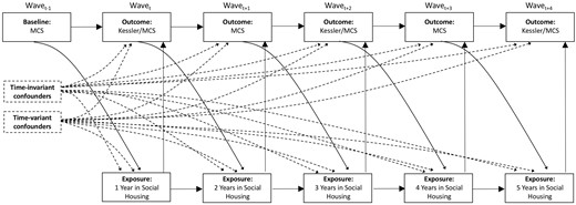
Directed acyclic graph (DAG).

Methods

Data source

The longitudinal Household, Income and Labour Dynamics in Australia Survey (HILDA) is a panel study of households. The outcome variable for this study, psychological distress as measured by the Kessler-10 (K10), was measured every second wave from 2009 to 2013, so we constructed three 5-year windows (2005–09 2007–11, 2009–13) with the last year of each window including the K10. Further, to examine a low-income cohort, we restricted participation to people residing in households in the lowest 40% of the income distribution in the first wave of each panel.

Housing exposure

The total number of years in social housing over five consecutive waves was constructed as both a categorical and a continuous variable ranging between 0 and 5. The number of transitions into and out of social housing, in each 5-year panel, was constructed as both a categorical and a continuous variable ranging from 0 to 4.

Mental health and psychological distress outcomes

We examined two mental health outcomes: (i) the mental health short-form summary score of the SF-36 (MH), ranging between 0 and 100 with increasing scores reflecting better mental health; and (ii) psychological distress, measured using the K10 ranging between 10 and 50 with lower score representing less psychological distress. Both were treated as continuous variables.

Potential confounders and time-varying variables affected by previous exposure

We included the following five time-invariant confounders: age (continuous), gender (female, male), country of birth (Australia, other English-speaking countries and other countries), Aboriginal or Torres Strait Islander status (yes, no) and highest educational qualification (graduate/postgraduate, high school/certificate, did not complete high school).

Poor mental health is plausibly related to social housing entry and pattern of occupancy, and (independent of social housing) future psychological distress and mental health. We included people’s MH score from the year preceding each panel (MH; continuous variable ranging from 0 and 100) as a time-invariant confounder.

In addition to including mental health as a baseline confounder, mental health in the year preceding each housing measure is also a time-varying mediator, as depicted in Figure 1. We therefore included lagged MH in the inverse probability weights generated for the MSMs.

At every wave, we included four time-varying confounders that we hypothesized were affected by housing status in the previous wave. These were household structure (couple with and without children, lone parent, lone person and other), equivalized household income (continuous measure adjusted for annual inflation), employment [employed, not in the labour force (NILF), unemployed] and long-term health condition (yes/no).

Statistical methods

Missing data

Data were missing in each of the 5-year window periods due to wave non-response and item non-response (Table 1). There was also data missing for the baseline MH score. Complete records were obtained for 45.6% of all participants included in the window 2005–09, 49.0% for 2007–11 and 48.0% for 2009–13.

Table 1.

Description of observed sample for 2005–09, 2007–11 and 2009–13

	2005–09		2007–11		2009–13
	n = 4788		n = 4999		n = 4543
Gende, (n, %)
Female	2625	54.8	2771	55.4	2515	55.4
Male	2163	45.2	2228	44.6	2028	44.6
Age (years; mean, SD)	48.94	21.4	48.23	21.5	49.36	21.9
Country of birth (n, %)
Australia	3461	72.3	3732	74.7	3358	73.9
Other main English-speaking	453	9.5	444	8.9	406	8.9
Other countries	662	13.8	648	12.9	631	13.9
Missing	212	4.4	175	3.5	148	3.3
Aboriginal/Torres Strait Islander (n, %)
Yes	207	4.3	245	4.9	241	5.3
Missing	212	4.4	175	3.5	148	3.3
Education (n, %)
High school/advanced certificate	1377	28.8	1567	31.4	1474	32.5
Graduate/postgraduate	650	13.6	717	14.3	636	14.0
Did not complete high school	2458	51.3	2455	49.1	2238	49.3
Missing	303	6.3	260	5.2	195	4.3
Household structure (n, %)
Couple with children	1489	31.1	1630	32.6	1272	28
Couple without children	1299	27.1	1305	26.1	1243	27.4
Lone parent	635	13.3	674	13.5	637	14.0
Lone person	1124	23.5	1130	22.6	1106	24.4
Other	241	5.0	260	5.2	285	6.3
Employment status (n, %)
Employed	1635	34.2	1865	37.3	1538	33.9
Not in the labour force	2623	54.8	2621	52.4	2553	56.2
Unemployed	227	4.8	253	5.1	257	5.7
Missing	303	6.3	260	5.2	195	4.3
Long-term health condition (n, %)
Yes	1887	39.4	1903	38.1	1902	41.9
Missing	304	6.4	260	5.2	200	4.4
Household income ($AUS, equivalized, CPI-adjusted) (n, mean)	16 293	4797.0	19 245	5958.7	21 070	7483.2
Mental health (SF36)
Mean, SD	71.84	18.6	71.6	18.7	71.76	18.9
Missing (n, %)	1128	23.6	1042	20.8	1208	26.6
Housing tenure (n, %)
Owner (outright and mortgage)	2900	60.6	2991	59.8	2611	57.5
Private renter	1089	22.7	1296	25.9	1200	26.4
Social renter	401	8.4	403	8.1	437	9.6
Other	394	8.2	306	6.1	273	6.0
Missing	4	0.1	3	0.1	22	0.5
Years in social housing (n, %)
0	3202	66.9	3487	69.7	3066	67.5
1	52	1.1	59	1.2	88	1.9
2	37	0.8	38	0.8	42	0.9
3	36	0.8	53	1.1	37	0.8
4	48	1	48	0.9	40	0.9
5	214	4.5	226	4.5	223	4.9
Missing	1199	25.0	1088	21.8	1047	23.1

To maximize information and minimize bias due to missing data, we performed multiple imputation through chained equations (MICE), using the R package MICE,¹² under the assumption that the data were missing at random (50 imputations using 50 cycles). Details of the imputation model and visual assessment of the imputed values are provided in Supplementary digital material, available as Supplementary data at IJE online. Complete-case analyses were performed as secondary analyses.

Marginal structural models

To deal with the time-varying confounders (listed above) and the strong pathway of mental health leading to social housing, and to estimate the causal effect of social housing on mental health, we used marginal structural models (MSMs).¹³ MSMs provide an unbiased average causal effect under the five assumptions of: (i) exchangeability (i.e. no unmeasured confounding); (ii) positivity (e.g. the existence of participants with 0 up to 5 years of social housing within strata of confounders); (iii) consistency (e.g. no variation in the quality of social housing and whether 2 or more years in social housing are consecutive or separated by time residing elsewhere); (iv) correct model(s) specification; and (v) no measurement error.

To reduce instability from small numbers of people making multiple transitions within a single 5-year window, we stacked the three panels before generating IPTWs (see below). We fitted an MSM by weighted linear regression of MH on number of years spent in social housing and number of social housing transitions made. We repeated the analysis with K10 as the outcome in the MSM, re-using the same non-truncated weights, so that exchangeability/probabilities incorporated a measure of mental health even though a K10 score was not available at each wave; that is, we used MH as the time-varying measure of mental health in the models where K10 (psychological distress) was the outcome variable at the fifth wave.

Construction of the inverse probability of treatment weighting

Inverse probability of treatment weights (IPTW) are a method to estimate the effect of time-dependent treatment (exposure) A_t whose value may depend on the treatment history (A_t-1, A_t-2, …, A₀) and on time-dependent covariates L_t that may themselves be influenced by the treatment history. For each wave in the analysis, the probability of observing the treatment A at time t for individual i was estimated using stabilized weights (SW):

$${SW}_{it}=\frac{p(A_{it}=a_{it}|{Ā}_{it-1}={ā}_{it-1})}{p(A_{it}=a_{it}|{Ā}_{it-1}={ā}_{it-1},{¯\mathit{L}}_{it}={¯\mathit{l}}_{it})}$$

Wherein:

ā_it = {a_it, a_it−1, … , a_i1}

The final weight is calculated by multiplying all the time-specific weights.

To maximize accuracy and precision of the weights, we used ensemble-learning methods.¹⁴ Specifically, we used the R package SuperLearner.¹⁵ In this approach, multiple models can independently be fitted to the same data, and the produced estimates can be combined into a weighted prediction. This approach allows automatic combination of the best features (accuracy of classification) of multiple types of base models (base learners) into a supermodel (Superlearner).

We tested three types of base learners: (i) a logistic regression model without interactions but including cubic b-splines of five degrees of freedom for the effect of age, MH at each wave and equivalized income at each wave; (ii) a gradient boosting machine (GBM); and (iii) a conditional inference forest. Both the GBM and conditional inference forest are decision-tree ensemble variations and are well described in Hothorn et al.¹⁶ and McCaffrey et al.¹⁷ We fitted MSMs using the weights estimated by each of these three base learners, as well as by the Superlearner that generates weighted averages from these three methods. The standardized mean differences between the exposed and unexposed, constituting balance diagnostics,¹⁸ for each potential confounder for the Superlearner approach are graphically presented in Supplementary Figure 2, available as Supplementary data at IJE online.

To address any remaining imbalance we fitted a ‘double robust’ linear model using both the IPTW and adjustment for baseline covariates age, gender, Indigeneity, employment status, presence of a long-term health condition and MH (see Supplementary Table 1, available as Supplementary data at IJE online).

Sensitivity analyses

To test how sensitive our findings were to the approach used to generate the IPTWs, we estimated an MSM where logistic regression was used to estimate IPTWs. We also estimated a model adjusted for previous cumulative exposure to social housing (for a restricted sample of respondents for whom this information was available) to gauge how much this source of residual confounding was likely to influence our findings.

To gauge the consequence of residual time-invariant confounding we sequentially added confounders to standard (non-IPTW) regression models: (i) age and sex; (ii) plus Indigenous status and country of birth; (iii) plus employment and education; (iv) plus baseline mental health, to determine attenuation from crude to fully time-invariant adjusted associations. A large attenuation, say over two-thirds, suggests that remaining (correlated) residual confounding or measurement error of included time-invariant confounders is responsible for any observed association.¹⁹

Results

Descriptive results

Table 1 shows the descriptive statistics for the observed data for each window. In each of the three analytical window samples 55% were female, and the mean age was between 48 and 49 years. The majority of participants were Australian-born (72–75%) and between 4% and 5% identified as Aboriginal or Torres Strait Islanders. Reflecting the low-income sample restriction, a significantly large proportion of people had not finished high school (29–32%) or were not in the labour force (52−56%); 38−42% reported having a long-term health condition. In terms of housing tenure, most people were outright owners and mortgage holders (ranging from 57% to 61% of the sample across the windows). Around 8% to 10% of the sample comprised social housing tenants at each window, with a significant number (ranging from 214 to 223) spending 5 years in social housing.

Figure 2 describes transitions, demonstrating that the majority of people who were in social housing in the first wave remained in social housing throughout the study period. Most transitions in and out of social housing were largely to and from private rental, and transitions to and from social housing and home ownership were less common again. To avoid clutter, only transitions between the same states, and to and from social housing, are shown. Transitions between private, owner/mortgage and other tenure are not shown. Only data in the first used imputed dataset per window are shown, and, these datasets were subsequently pooled across the windows.

Figure 2.

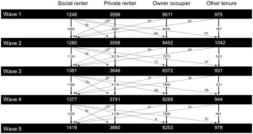
Transitions into and out of social housing in each panel.

Analytical results

Cumulative effect of years in social housing

When cumulative exposure to social housing was modelled as a categorical variable (Table 2), there was evidence of worsening of mental health across both K10 and MH measures with each additional year in public housing up to 4 years (compared with no years of social housing). People in 5 years of social housing, that is people who did not make a housing transition throughout the panel, had worse mental health than people who had no exposure to social housing; however, their mental health was not as bad, on average, as people who had made some form of social housing transition.

Table 2.

Cumulative exposure to social housing and social housing transitions in relation to measures of mental health and psychological distress

Social housing		MH estimate [95% confidence interval]	K10 estimate [95% confidence interval]
Categorical
Cumulative	0	Ref	Ref
	1	−0.37 [−2.70; 1.96]	0.14 [−0.74; 1.01]
	2	−2.54 [−6.16; 1.09]	0.77 [−0.55; 2.08]
	3	−3.32 [−7.13; 0.50]	2.20 [0.56; 3.84]
	4	−2.76 [−6.48; 0.96]	1.03 [−0.47; 2.53]
	5	−1.91 [−3.42; −0.39]	0.94 [0.35; 1.54]
Transitions	0	Ref	Ref
	1	−1.55 [−3.75; 0.65]	0.50 [−0.43; 1.44]
	2	−2.19 [−5.27; 0.89]	1.02 [−0.18; 2.21]
	3	−2.03 [−7.90; 3.84]	1.95 [−0.35; 4.26]
	4	−5.85 [−25.37; 13.67]	4.17 [−4.12; 12.46]
Continuous
Number of transitions		−1.04 [−2.16; 0.09]	0.56 [0.12; 1.00]

When the number of social housing transitions over each 5-year panel was modelled categorically (Table 2 and Figure 3), there is evidence of a nearly monotonic effect of social housing transitions on the MH measure (i.e. slight drop from −2.19 to −2.03 for two to three transitions), and monotonic for K10. Supplementary Figure 2 graphically shows these estimates, but for purposes of comparison the K10 has been rescaled from 0 to 100 and converted to the same negative direction as the MH; there is consistency between the MH and K10 results.

Figure 3.

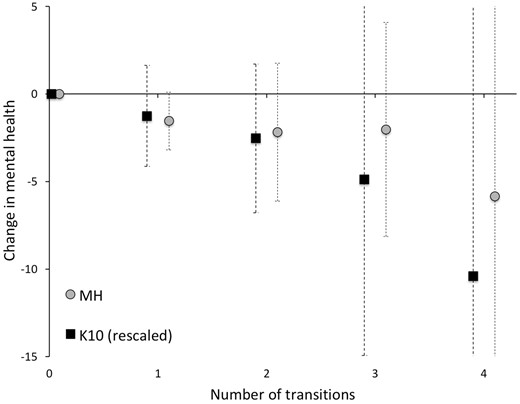
Estimates of the association between number of social housing transitions and mental health with 95% confidence intervals.

Given monotonicity, we fitted a linear association of the number of transitions as a continuous variable (Table 2), finding worsening mental health with each additional social housing transition made: -1.04 [95% confidence interval (CI) −2.16; 0.09] for the MH and 0.56 (95% CI 0.13; 1.00) for the K10. The change in MH is in the order of 6% of one standard deviation and of K10 is 9% of one standard deviation, thus three transitions compared with none are associated with an approximately 18% of a standard deviation in worsening of mental health and 27% standard deviation in worsening of psychological distress.

Sensitivity analyses

We generated estimates from MSMs using complete cases only. The pattern of results is broadly similar to estimates obtained from MSMs using multiple imputation for handling the missing data (Supplementary Table 2, available as Supplementary data at IJE online). We also estimated IPTW weights using logistic regression (Supplementary Table 2, available as Supplementary data at IJE online). This approach generated wider confidence intervals and worse balance across covariates (Supplementary Figures 1 and 2, available as Supplementary data at IJE online),

We restricted the dataset to people whose housing history in the 3 years preceding each panel was known (reducing the sample by 16%) so as to estimate models with and without adjustment for previous cumulative exposure to social housing (Supplementary Table 3, available as Supplementary data at IJE online). The strength of association of cumulative housing with mental health increased modestly when adjusting for previous cumulative housing, and the association of transitions into and out of social housing with mental health decreased modestly.

Finally, when we set IPTW weights aside and estimated the change in strength of association from crude to fully adjusted for time-invariant confounders, there was sizeable attenuation of estimates for cumulative exposure (0 vs 5 years) and transitions for each outcome (Supplementary Table 4, available as Supplementary data at IJE online; see Discussion).

Discussion

In an era of widespread changes to the role and provision of social housing,^3,4,20,21 this study has sought to answer two important questions on the mental health effects of cumulative exposure to social housing and social housing transitions. We found that people with no exposure to social housing report better mental health and less psychological distress than people who spend consecutive, cumulative time in social housing over a 5-year period. We also observed a negative effect on mental health of transitions into and out of socially provided housing, such that mental health worsened and psychological distress increased nearly monotonically with each additional transition. These findings remain important against a backdrop of the gradual introduction of fixed term, rather than lifetime, leases in the social housing sector across many high- and middle-income countries.⁵

We acknowledge a number of important limitations of these analyses. We thoroughly address time-varying covariates. We also adjusted for measured time-invariant confounders (including baseline mental health) both through the IPTWs and doubly robust adjustment in the MSM, and sensitivity analyses adjusting for previous social housing (although diminishing statistical power) did not overturn conclusions. However, as with most observational studies of this type, remaining residual confounding by time-invariant confounders remains a concern. In our sensitivity analyses determining the attenuation of effect by just adjusting for measured time-invariant confounders (Supplementary Table 4, available as Supplementary data at IJE online; e.g. education, previous mental health), we found large attenuation from the crude to adjusted analyses; it therefore remains possible that better measurement of time-invariant confounders could have driven our findings to the null. It must be noted that this caveat applies to most observational studies.

Second, there were a relatively small number of social housing transitions in our sample over the 5-year windows (as described Figure 1). Nonetheless, this is still the largest study to examine cumulative exposure to social housing and the ‘churn’ of transitions. Third, as with similar studies that use self-reported health outcomes, we note that they may be vulnerable to measurement error; however, baseline adjustment for mental health should ameliorate this to some extent if within-individual measurement error is stable over time. Fourth, our reference group necessarily contains a mix of private renters and owners/mortgagees in order to capture people’s movement into and out of social housing from a variety of tenures. This creates unavoidable heterogeneity in our reference group. Fifth, it is important to acknowledge that, as with the owned and privately rented housing sectors, there may be qualitative differences in the condition of social housing across jurisdictions. This limits to an unknown extent the generalizability of our findings. Finally, we have only considered social housing transitions in this paper, and do not know the comparative impact of transitions between other tenures on mental health and psychological distress.

Despite these limitations, this paper has important strengths. It is among the few to causally examine the effect of social housing on mental health.²² It uses nationally representative panel data and a rigorous suite of methods to address confounding and improve performance, including MSMs to account for the complexities of time-varying confounding, ensemble learning to improve prediction of IPTWs, double robust adjustment for baseline covariates to reduce residual confounding, multiple imputation to address missing data, and adjustment for previous social housing exposure and baseline mental health to address selection. This is the best we can do given it is not be feasible to conduct a randomized trial on this population.

Across many similar nations, social housing is a key welfare response specifically targeted to a high-needs population, making social housing tenants one of the most policy-important population groups. This study provides evidence that, although long periods of time in social housing are associated with worse mental health, housing stability may ensure better mental health outcomes for social housing tenants, with those who make the most transitions in the 5-year window having considerably worse mental health profiles than those who maintain stability of tenure in social housing.

Access to the Household, Income and Labour Dynamics in Australia survey is available to approved researchers by application to Melbourne Institute, University of Melbourne. The code in R used to run these models is available upon request from the authors.

Funding

R.B. and E.B. are funded by Australian Research Council (ARC) Future Fellowships (FT150100131 and FT1401100872 respectively). J.S. is funded by a National Health and Medical Research Council (NHMRC) Senior Research Fellowship (1104975). T.B. receives funding through the Burden of Disease Epidemiology, Equity and Cost-Effectiveness Programme, Health Research Council of New Zealand (16/443).

Acknowledgements

We would like to acknowledge the contribution of Frank Pega to the early conceptualization of these analyses. This paper uses unit record data from the Household, Income and Labour Dynamics in Australia (HILDA) Survey. The HILDA Project was initiated and is funded by the Australian Government Department of Social Services (DSS) and is managed by the Melbourne Institute of Applied Economic and Social Research (Melbourne Institute). The findings and views reported in this paper, however, are those of the authors and should not be attributed to either the DSS or the Melbourne Institute.

Conflict of interest: None to declare.

Author notes

Co-senior authors of this paper.