Fluid dynamics in heart development: effects of hematocrit and trabeculation

Abstract

Recent in vivo experiments have illustrated the importance of understanding the haemodynamics of heart morphogenesis. In particular, ventricular trabeculation is governed by a delicate interaction between haemodynamic forces, myocardial activity, and morphogen gradients, all of which are coupled to genetic regulatory networks. The underlying haemodynamics at the stage of development in which the trabeculae form is particularly complex, given the balance between inertial and viscous forces. Small perturbations in the geometry, scale, and steadiness of the flow can lead to changes in the overall flow structures and chemical morphogen gradients, including the local direction of flow, the transport of morphogens, and the formation of vortices. The immersed boundary method was used to solve the two-dimensional fluid-structure interaction problem of fluid flow moving through a two chambered heart of a zebrafish (Danio rerio), with a trabeculated ventricle, at 96 hours post fertilization (hpf). Trabeculae heights and hematocrit were varied, and simulations were conducted for two orders of magnitude of Womersley number, extending beyond the biologically relevant range (0.2–12.0). Both intracardial and intertrabecular vortices formed in the ventricle for biologically relevant parameter values. The bifurcation from smooth streaming flow to vortical flow depends upon the trabeculae geometry, hematocrit, and Womersley number, |$Wo$|⁠. This work shows the importance of hematocrit and geometry in determining the bulk flow patterns in the heart at this stage of development.

immersed boundary method, heart development, trabeculation, hematocrit, fluid dynamics, haemodynamics

1. Introduction

Fluid dynamics is important to organogenesis in many systems. The advection and diffusion of morphogens as well as the haemodynamic forces generated are known to regulate morphogenesis (Patterson, 2005). Forces such as shear stress and pressure may be key components that activate developmental regulatory networks (Tarbell et al., 2005). These mechanical forces act on the cardiac cells, where the mechanical stimuli is then transmitted to the interior of the cell via intracellular signalling pathways, i.e. mechanotransduction. In terms of mixing, the magnitude, direction, and pulsatile behaviour of flow near the endothelial layer may influence receptor-ligand bond formation (Taylor et al., 1996) and enhance the mixing of chemical morphogens. Advection-driven chemical gradients act as epigenetic signals driving morphogenesis in ciliary-driven flows (Cartwright et al., 2009; Freund et al., 2012), and it is possible that flow-driven gradients near the endothelial surface layer also play a role in cardiogenesis and vasculogenesis.

The notion that flow is essential for proper vertebrate cardiogenesis is not a recent idea. It was first investigated by Chapman in 1918 when chicken hearts were surgically dissected during embryogenesis, and their resulting circulatory systems did not develop properly (Chapman, 1918). Moreover, the absence of erythrocytes at the initiation of the first heart beat and for a period of time later, supports the belief that the early developing heart does not pump for nutrient transport. These results suggest that the function of the embryonic heart is to aid in its own growth as well as that of the circulatory system (Burggren, 2004).

Later experiments show that obstructing flow in the venous inflow tract of developing hearts in vivo results in problems in proper chamber and valve morphogenesis (Hove et al., 2003; Stekelenburg-de Vos et al., 2003; Gruber & Epstein, 2004). For example, Gruber & Epstein (2004) found that irregular blood flow can lead to hypoplastic left heart syndrome (HLHS), where the ventricle is too small or absent during the remainder of cardiogenesis. Hove et al. (2003) observed that when inflow and outflow tracts are obstructed in 37 hours post fertilization (hpf) zebrafish, regular waves of myocardial contractions continue to persist and neither valvulogenesis, cardiac looping, nor chamber ballooning occur. Similarly, Stekelenburg-de Vos et al. (2003) performed a similar experiment in chicken embryos at a similar morphological stage of development, e.g. HH-stage 17 (Hamburger & Hamilton, 1951; Martinsen, 2005), whereby the venous inflow tract was obstructed temporarily. They noticed that all haemodynamic parameters decreased initially, i.e. heart rate, peak systolic velocity, time-averaged velocity, peak and mean volumetric flow, and stroke volume. Only the heart rate, time-averaged velocity, and mean volumetric flow recovered near baseline levels.

Trabeculae are particularly sensitive to changes in intracardiac haemodynamics (Granados-Rivero & Brook, 2012). Trabeculae are bundles of muscle that protrude from the interior walls of the ventricles of the heart. The sensitivity of the trabeculae under varying mechanical loads is important when considering they may serve as important structures in which cellular mechanotransduction occurs. Trabeculation may also help regulate and distribute shear stress over the ventricular endocardium, enhance mixing and modify chemical morphogen gradients. Furthermore, the presence of trabeculation may contribute to a more uniform transmural stress distribution over the cardiac wall (Malone et al., 2007). Even subtle trabeculation defects arising from slight modifications in haemodynamics may magnify over time. As the mechanical force distribution changes due to the absence of normal trabeculae, Neuregulin signalling, along with other genetic signals, are disrupted, leading to further deviations from healthy cardiogenesis. For example, zebrafish embryos that are deficient in the key Neuregulin co-receptor ErbB2 display severe cardiovascular defects including bradycardia, decreased fractional shortening, and impaired cardiac conduction (Liu et al., 2010). Disrupted shear distributions in the ventricle leads to immature myocardial activation patterns, which perpetuate ventricular conduction and contractile deficiencies, i.e. arrhythmia, abnormal fractional shortening and possibly ventricular fibrillation (Reckova et al., 2003).

The fluid dynamics of heart development, particularly at the stage when the trabeculae form, is complex due to the balance of inertial and viscous forces. The Reynolds number, |$Re$| is a dimensionless number that describes the ratio of inertial to viscous forces in the fluid and is given as |$Re = (\rho U L)/\mu$|⁠. In cardiac applications, |$\mu$| is the viscosity of the blood, |$\rho$| is the density of the blood, |$U$| is the characteristic velocity (often chosen as the average or peak flow rate) and |$L$| is the characteristic length (often chosen as the diameter of the chamber or vessel). Another dimensionless parameter that is often used in describing cardiac flows is the Womersley number which is given by |$Wo = \frac{2\pi f L^2}{\nu}$|⁠, where |$f$| is the frequency of contraction and |$\nu=\frac{\mu}{\rho}$| is the kinematic viscosity. Note that the |$Wo$| describes the transient inertial force over the viscous force and is a measure of the importance of unsteadiness in the fluid. During critical developmental stages such as cardiac looping and the formation of the trabeculae, |$Re \approx 1$| and |$Wo \approx 1$|⁠. In this regime, a number of fluid dynamic transitions can occur, such as the onset of vortical flow and changes in flow direction, that depend upon the morphology, size of the chambers and effective viscosity of the blood. The flow is also unsteady, and the elastic walls of the heart undergo large deformations.

Since analytical solutions are not readily available for complex geometries at intermediate |$Re$|⁠, recent work has used computational fluid dynamics (CFD) to resolve the flow in the embryonic heart. For example, DeGroff et al. (2003) reconstructed the 3D surface of human heart embryo using a sequence of 2D cross-sectional images at stages 10 and 11, when the heart is mere valveless tube (Hill, 2017). The cardiac wall was fixed, and steady and pulsatile flows were driven through the chambers. They found streaming flows (particles released on one side of the lumen did not cross over or mix with particles released from the opposite side) without coherent vortex structures. Liu et al. (2007) simulated flow through a three-dimensional model of a chick embryonic heart during stage HH-21 (after about 3.5 days of incubation) at a maximum |$Re$| of about 6.9. They found that vortices formed during the ejection phase near the inner curvature of the outflow tract. More recently, Lee et al. (2013) performed 2D simulations of the developing zebrafish heart with moving cardiac walls. They found unsteady vortices develop during atrial relaxation at 20–30 hpf and in both the atrium and ventricle at 110–120 hpf. Goenezen et al. (2016) used subject-specific CFD to model flow through a model of the chick embryonic heart outflow tract.

The numerical work described above, in addition to direct in vivo measurements of blood flow in the embryonic heart (Hove et al., 2003; Vennemann et al., 2006), further supports that the presence of vortices is sensitive to changes in |$Re$|⁠, morphology, and unsteadiness of the flow. Santhanakrishnan et al. (2009) used a combination of CFD and flow visualization in dynamically scaled physical models to describe the fluid dynamic transitions that occur as the chambers balloon, the endocardial cushions grow, and the overall scale of the heart increases. They found that the formation of intracardial vortices depended upon the height of the endocardial cushions, the depth of the chambers, and the |$Re$|⁠. Their paper only considers steady flows in an idealized two-dimensional chamber geometry with smooth, stationary walls.

In this article, we quantify the kinematics of the two-chambered zebrafish heart at 96 hpf and use that data to construct both the geometry and prescribed pumping motion of a two-chambered heart computational model. We use the immersed boundary method to solve the fluid-structure interaction problem of flow through a two-chambered pumping heart. The model we develop prescribes the pumping motion of the chambers, based on kinematic data taken from in vivo 2D cross-sectional temporally-sliced images of a zebrafish heart at 4 days post fertilization (dpf) from Liu et al. (2010). The goal of this paper is to discern bifurcations in the intracardial and intertrabecular flow structures due to scale (⁠|$Wo$|⁠), trabeculae height and hematocrit. We find a variety of interesting bifurcations in flow structures that occur over a biologically relevant morphospace. The implications of the work are that alterations in bulk flow patterns, and particularly the presence or absence of intracardial and intertrabecular vortices, will augment or reduce mixing in the heart, alter the direction and magnitude of flow near the endothelial surface layer, and potentially change chemical gradients of morphogens which serve as an epigenetic signal.

2. Numerical method

2.1 Model geometry

A simplified two dimensional geometry of a 96 hpf zebrafish’s two-chambered heart, containing trabeculae, was constructed using Fig. 1(a,b). The ventricle and atrium were idealized as an ellipse, with semi-major axis |$V_a$|⁠, and |$A_a$|⁠, and semi-minor axis |$V_b$| and |$A_b$|⁠, respectively. The atrioventricular canal (AV canal) connects the atrium and ventricle and is modelled as endocardial cushions, which move to occlude or promote flow through the heart chambers. The sinus venosus (SV) and bulbus arteriosus (BA) are modelled similarly. The width of the AV canal, SV and BA are given by |$w_{AV}, w_{SV}$| and |$w_{BA}$|⁠, respectively. The above parameters are labelled systole and diastole separately, e.g. the ventricular subscripts are given an |$exp$| label right before systole and are labelled |$con$| before diastole, while the atrial labels are opposite.

Fig. 1.

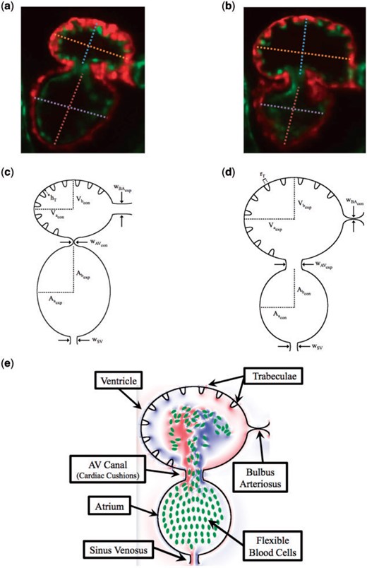
(a, b) Snapshots of an embryonic zebrafish’s ventricle at 96 hpf right using spinning disk confocal microscopy. The snapshots were taken right before its diastolic and systolic phase, respectively. The protrusions into the ventricular chamber are trabeculae. Dashed lines show the minor and major axes. Images are from Tg(cmlc2:dsRed)s879; Tg(flk1:mcherry)s843 embryos expressing fluorescent proteins that label the myocardium and endocardium, respectively (Liu et al., 2010). The red fluoresces the myocardium, while the green fluoresces the endocardium. (c, d) illustrate the computational geometry right before diastole and systole, respectively. The computational geometry, as shown in (e), includes the two chambers, the atrium (bottom chamber) and ventricle (top chamber), the atrioventricular canal connecting the chambers and the bulbus arteriosus and sinus venosus, which all have endocardial cushions, which can occlude cardiac flow, as well as flexible blood cells.

Elliptical blood cells of uniform semi-major and semi-minor axis lengths, |$C_a$| and |$C_b$|⁠, respectively, were included. The volume fraction, or hematocrit, was varied between |$[0\%, 25\%]$|⁠. Hematocrit increases linearly throughout development (Al-Roubaie et al., 2011) from |$0\%$| to roughly |$32\%$| (Eames et al., 2010). The desired volume fraction of blood cells was calculated within the atrium, and the blood cells were spaced evenly apart within it. Moreover, as the ejection fraction is |$60\%$| (Forouhar et al., 2006), |$60\%$| of the number of blood cells in the atrium were spaced evenly within the ventricle. in vivo images from Liu et al. (2010) are shown in Fig. 2. Note that this placement of blood cells occurred immediately before diastole.

Fig. 2.

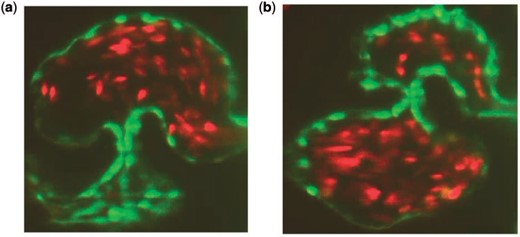
(a, b) Snapshots of an embryonic zebrafish’s ventricle at 96 hpf right using spinning disk confocal microscopy. The snapshots were taken right before systole and diastole, respectively. The protrusions into the ventricular chamber are trabeculae and blood cells are fluorescing red (Liu et al., 2010).

The trabeculae geometry was modelled using the following perturbed Gaussian-like function,

\begin{equation} T(x) = h_T \left(1 - \left(\frac{x}{r_T}\right)^2 \right) e^{-\left(\frac{x}{0.7r_T} \right)^8 }, \end{equation}

(1)

where |$r_T$| and |$h_T$| are the radii and height of each trabecula, respectively, and |$x\in[-r_T,r_T]$|⁠. Trabeculae are placed equidistant, as estimated from Fig. 1(a,b). The full geometry can be seen in Fig. 1. Each trabeculae in this model is filled with fluid that has same physical properties as the fluid elsewhere.

The blood cells were approximated as ellipses, using Figure 2 to estimate their length to width ratios, with respect to the size of the ventricle. The blood cells were held nearly rigid, as described in Section 2.2.

The dimensionless geometric model parameters are found in Table 1, which were scaled from measurements taken from Fig. 1(a,b). The radii, |$r_T$|⁠, and number of the trabeculae were constant in all numerical simulations, while the height of the trabeculae, |$h_T$|⁠, was varied.

Table 1

Table of dimensionless geometric parameters used in the numerical model. The non-dimensionalization was done by dividing by |$V_{\rm a_{exp}}$|⁠. The height of trabeculae, |$h_T$|⁠, were varied for numerical experiments

Parameter	Symbol	Value
Contracted ventricle semi-major axis	|$V_{\rm a_{con}}$|	0.80
Contracted atrium semi-major axis	|$A_{\rm a_{con}}$|	0.68
Contracted ventricle semi-major axis	|$V_{rm _{con}}$|	0.64
Contracted atrium semi-major axis	|$A_{\rm b_{con}}$|	0.76
Expanded ventricle semi-major axis	|$V_{\rm a_{exp}}$|	1.00
Expanded atrium semi-major axis	|$A_{\rm a_{exp}}$|	0.88
Expanded ventricle semi-major axis	|$V_{\rm b_{exp}}$|	0.84
Expanded atrium semi-major axis	|$A_{\rm b_{exp}}$|	1.02
Contracted AV-canal width	|$w_{\rm AV_{con}}$|	0.02
Contracted bulbus arteriosus width	|$w_{\rm BA_{con}}$|	0.015
Open AV-canal width	|$w_{\rm AV_{exp}}$|	0.34
Open bulbus arteriosus width	|$w_{\rm BA_{exp}}$|	0.29
Sinus venosus width	|$w_{\rm SV}$|	0.2
Blood cell semi-major axis	|$C_a$|	0.050
Blood cell semi-major axis	|$C_b$|	0.025
Trabeculae radii	|$r_T$|	0.06
Trabeculae height	|$h_T$|	|$\{0, 0.09, 0.18, 0.27, 0.36\}$|

2.2 Numerical method

The immersed boundary method (Peskin, 2002) was used to solve for the flow velocities within the geometric model from Section 2.1. The immersed boundary method has been successfully used to study the fluid dynamics of a variety of biological problems in the intermediate Reynolds number range, defined here as |$0.01<Re<1000$| (see, for example, (Jung, 2001; Tytell et al., 2010; Hershlag & Miller, 2011; Bhalla et al., 2013). The model consists of stiff boundaries that are immersed within an incompressible fluid of dynamic viscosity, |$\mu$| and density, |$\rho$|⁠. The fluid motion is described using the full 2D Navier–Stokes equations given as

\begin{gather} \rho \left( \frac{\partial {\bf{u}}({\bf{x}},t) }{\partial t} + {\bf{u}}({\bf{x}},t)\cdot \nabla {\bf{u}}({\bf{x}},t) \right) = -\nabla p({\bf{x}},t) + \mu \Delta {\bf{u}}({\bf{x}},t) + {\bf{F}}({\bf{x}},t) \\ \end{gather}

(2)

\begin{gather} \nabla\cdot {\bf{u}}({\bf{x}},t) = 0, \end{gather}

(3)

where |${\bf{u}}({\bf{x}},t) = (u({\bf{x}},t),v({\bf{x}},t))$| is the fluid velocity, |$p(\bf{x},t)$| is the pressure, |${\bf{F}}({\bf{x}},t)$| is the force per unit volume (area in |$2D$|⁠) applied to the fluid by the immersed boundary, i.e. two-chambered heart. The independent variables are the position, |${{\bf{x}}}= (x,y)$|⁠, and time, |$t$|⁠. Equation (2) is equivalent to the conservation of momentum for a fluid, while (3) is a condition mandating that the fluid is incompressible.

The interaction equations between the fluid and the immersed structure are given by

\begin{gather} {\bf{F}}({\bf{x}},t) = \int {\bf{f}}(r,t)\delta({\bf{x}}-{\bf{X}}(r,t)) dr\\ \end{gather}

(4)

\begin{gather} {\bf{U}}({\bf{X}}(r,t),t) = \frac{\partial {\bf{X}}(r,t)}{\partial t} = \int {\bf{u}}({\bf{x}},t) \delta( {\bf{x}} - {\bf{X}}(r,t) ) d{\bf{x}}, \end{gather}

(5)

where |${\bf{X}}(r,t)$| gives the Cartesian coordinates at time |$t$| of the material point labelled by Lagrangian parameter |$r$|⁠, |${\bf{f}}(r,t)$| is the force per unit area imposed onto the fluid by elastic deformations in the boundary, as a function of the Lagrangian position, |$r$|⁠, and time, |$t$|⁠. Equation (4) applies a force from the immersed boundary to the fluid grid through a delta-kernel integral transformation. Equation (5) sets the velocity of the boundary equal to the local fluid velocity.

The regularized delta function used in (4) and (5) is defined as

\begin{equation} \delta_h(\textbf{x}) = \delta_h(x)\delta_h(y), \end{equation}

(6)

where |$\delta_h(x) = \frac{1}{h} \psi\left(\frac{x}{h}\right)$| and |$\psi(r)$| is the four-point function described in Peskin (2002),

\begin{equation} \psi(r) = \left\{ \begin{array}{l} \frac{1}{8}(3-2|r|+\sqrt{1+4|r|-4r^2} ) \ \ \ \ 0\leq |r| < 1 \\ \frac{1}{8}(5-2|r|+\sqrt{-7+12|r|-4r^2}) \ \ \ \ 1\leq|r|<2 \\ 0 \ \ \ \ \ \ \ \ \ \ \ \ \ \ \ \ \ \ \ \ \ \ \ \ 2\leq |r|.\\ \end{array}\right. \end{equation}

(7)

This regularized delta function is used to both spread the force from the Lagrangian force density of the curvilinear mesh onto the Cartesian fluid grid, (4), and to interpolate the velocity onto the Lagrangian mesh based from the underlying local fluid velocity of the Cartesian grid, (5).

The force equations are specific to the application. In a simple case where a preferred motion or position is enforced, boundary points are tethered to target points via springs. The equation describing the force applied to the fluid by the boundary in Lagrangian coordinates is given by |${\bf{f}}(r,t)$| and is explicitly written as,

\begin{equation} {\bf{f}}_{\rm trgt}(r,t) = k_{\rm target} \left( {\bf{Y}}(r,t) - {\bf{X}}(r,t) \right)\!, \end{equation}

(8)

where |$k_{\rm target}$| is the stiffness coefficient, and |$\textbf{Y}(r,t)$| is the preferred Lagrangian position of the target structure. In all simulations the motion of the two-chambered heart (atrium, the trabeculated ventricle, AV canal, SV and BA) was prescribed by applying a force proportional to the distance between location of the actual boundary and the preferred position. The deviation between the actual and preferred positions can be controlled with the variable |$k_{target}$|⁠.

The blood cells’ deformations and movement was governed by fully coupled fluid-structure interaction and movement was not prescribed. Linear springs were used to model the flexibility of blood cells; however, the spring stiffnesses were large as only to allow negligible deformations. Springs were attached between both adjacent Lagrangian points as well as the Lagrangian point across from them. The forces applied to the fluid from deformations of the blood cells is given by

\begin{equation} {\bf{f}}_{\rm spr}(r,t) = k_{\rm spring} \left( 1 - \frac{R_L}{||{\bf{X}}_{SL}(r,t)-{\bf{X}}_{M}(r,t)||} \right) \cdot \left( \begin{array}{c} x_{SL} - x_M \\ y_{SL} - y_M \end{array} \right)\!, \end{equation}

(9)

where |${\bf{X}}_{M}$| and |${\bf{X}}_{SL}$| give the positions in Cartesian coordinates of the master and slave nodes, respectively, |$k_{\rm spring}$| is the spring stiffness, and |$R_L$| is the resting length of the spring. In this formulation, the master and spring node will undergo the same deformation force, but in opposite directions. Deformable blood cells have been modelled using immersed boundary framework previously (Crowl & Fogelson, 2009, 2011); however those studies were not in the vein of embryonic cardiac flows.

2.3 Prescribed motion of the two chambers

The motion of the two-chambered heart was modelled after a video taken using spinning disk confocal microscopy from Liu et al. (2010) of a wild-type zebrafish embryo at |$96 $| hpf. The video’s images were acquired with a Nikon Te-2000u microscope (Nikon) at a rate of 250 frames per second using a high-speed CMOS camera (MiCam Ultima, SciMedia) (Liu et al., 2010). Using the MATLAB software package DLTdv (Hedrick, 2008), the systolic and diastolic periods were determined by measuring maximum width and height of both the atrial and ventricular chambers. These results are shown in Fig. 3(a,b). The maximum width of the AV canal was also measured in pixels right before diastole, and found to be |$25$| pixels. Assuming the width of the AV canal is |$42\, \mu m$| (Forouhar et al., 2006), each single pixel corresponds to |$1.68 \, \mu m.$| The converted height and widths in |$\mu m$| are found in Table 2. The average heights and radii of the trabeculae were found to be |$20.96\, \mu m$| and |$7.29\, \mu m$|⁠, respectively.

Fig. 3.

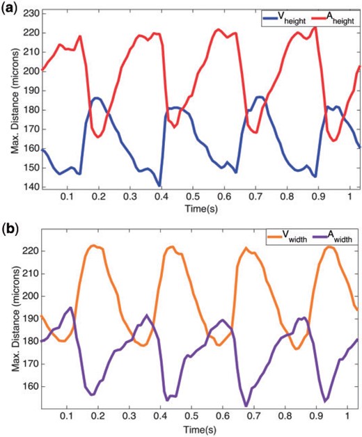
(a, b) Illustrate the maximum distance for the height and width (in pixels) respectively, in the atrium and ventricle of a 4 dpf embryonic zebrafish heart from Liu et al. (2010).

Table 2

The morphological parameters in physical units as computed from the kinematic analysis.

Ventricular parameters		Atriuml parameters		Trabecular parameters
Parameter	Max. length (⁠|$\mu m$|⁠)	Parameter	Max. length (⁠|$\mu m$|⁠)	Parameter	Length (⁠|$\mu m$|⁠)
|$\tilde{V}_{\rm a_{con}}$|	89.20	|$\tilde{A}_{\rm a_{exp}}$|	98.11	|$\tilde{r}_T$|	7.29
|$\tilde{V}_{\rm b_{con}}$|	70.84	|$\tilde{A}_{\rm b_{exp}}$|	113.11	|$\tilde{h}_T$|	20.97
|$\tilde{V}_{\rm a_{exp}}$|	111.98	|$\tilde{A}_{\rm a_{con}}$|	76.59
|$\tilde{V}_{\rm b_{exp}}$|	93.78	|$\tilde{A}_{\rm b_{con}}$|	84.10

One entire heart cycle was found to take place in approximately |$27$| frames. Assuming the heart beat frequency is |$3.95\ \rm beats/s$| (Malone et al., 2007), each pumping cycle lasts |$\sim0.25\,\rm s$|⁠. Each heart chamber undergoes four phases during each cycle: a rest period at the end of contraction, a period of expansion, a rest period at the end of expansion, and a period of contraction. The average percentage and duration of each phase are given in Table 3.

Table 3

Average percentage and duration of each phase during the heart cycle obtained from kinematic analysis.

Ventricular phases			Atrial phases
Phase	% of period	Time (s)	Phase	% of period	Time (s)
Rest after contraction	20.7	0.05	Rest after expansion	20.7	0.05
Expansion	24.0	0.06	Contraction	24.0	0.06
Rest after expansion	7.9	0.02	Rest after contraction	2.2	0.01
Contraction	47.4	0.12	Expansion	53.1	0.13

The prescribed motion of the two-chamber hearts was performed by interpolating between different phases of the heart cycle. This is illustrated in Fig. 4 which show the beginning of each phase. Phase 1: the ventricle rests after contraction and the atrium rests after expansion. The AV canal goes from fully occluded to |$10\%$| occlusion. Phase 2: The diastolic phase when the ventricle expands while the atrium contracts. Phase 3: the ventricle rests after expansion and the atrium rests after contraction. The AV canal becomes fully occluded state. Phase 4: The systolic phase, when the ventricle contracts and the atrium expands. Note we model the time in each phase after the ventricle motion, only. Moreover, note in each phase the volume within each trabeculae remains the same.

Fig. 4.

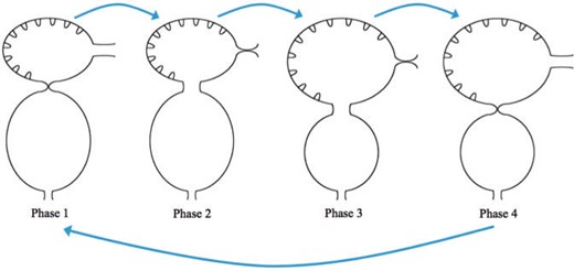
We describe four phases of each heart cycle. Note that the position at the beginning of each phase is shown. Phase 1: the ventricle rests after contraction and the atrium rests after expansion. The AV canal goes from fully occluded to |$10\%$| occlusion. Phase 2: The diastolic phase when the ventricle expands while the atrium contracts. Phase 3: the ventricle rests after expansion and the atrium rests after contraction. The AV canal becomes fully occluded state. Phase 4: The systolic phase, when the ventricle contracts and the atrium expands.

The actual motion of the heart is driven by changing the preferred position of the target points. Each phase transition used the following interpolation function,

$$ {\bf{X}}_{\rm target} = {\bf{X}}_{\rm current} + g_j(t)\left[ {\bf{X}}_{\rm next} - {\bf{X}}_{\rm current} \right]\!, $$

where |${\bf{X}}_{\rm current}$| is the current phase |$(X,Y)$|- positions of the Lagrangian structure, and |${\bf{X}}_{\rm next}$| are the |$(X,Y)$|-coordinates for the next phase of the heart cycle. Note that the target position, |${\bf{X}}_{\rm target}$|⁠, is |$\textbf{Y}(r,t)$| from (8). This initializes a penalty force to drive the Lagrangian structure towards its preferred position at each time-step, where the preferred position is the interpolated position between the current phase and next phase, shown in Fig. 4. The interpolation function, |$g_j(t)$| is defined below,

\begin{equation} g_j(t) = \left\{ \begin{array}{ll}\displaystyle c_1 \left( \frac{t}{T_{P_j}} \right)^2 & t<t_1 \\ \displaystyle c_3\left(\frac{t}{T_{P_j}}\right)^3 + c_4\left( \frac{t}{T_{P_j}}\right)^2 + c_5\left(\frac{t}{T_{P_j}}\right) + c_6 & t_1\leq t \leq t_2 \\ \displaystyle -c_2 \left( \frac{t}{T_{P_j}}-1 \right)^2 + 1 & t>t_2, \end{array}\right. \end{equation}

(10)

where |$T_{P_j}$| is the total time for Phase |$j$|⁠. Equation (10) was chosen to enforce continuous accelerations between phases. The coefficients |$\{c_k\}_{k=1}^{6}$| are given in Table 4 and the durations of each phase are reported in Table 5.

Table 4

Table of polynomial coefficients for the interpolating function, |$g_j(t)$|

Parameter	Value
|$c_1$|	2.739726027397260
|$c_2$|	2.739726027397260
|$c_3$|	|$-$|2.029426686960933
|$c_4$|	3.044140030441400
|$c_5$|	|$-$|0.015220700152207
|$c_6$|	0.000253678335870

Table 5

Table of temporal parameters used in the interpolating function, |$g_j(t)$|

Phase 1		Phase 2
Parameter	Time	Parameter	Time
|$T_P$|	|$0.207\times$| Period	|$T_P$|	|$0.240\times$| Period
|$t_1$|	|$0.05\times T_{P_1}$|	|$t_1$|	|$0.07\times T_{P_2}$|
|$t_2$|	|$0.95\times T_{P_1}$|	|$t_2$|	|$0.93\times T_{P_2}$|
Phase 3		Phase 4
Parameter	Time	Parameter	Time
|$T_P$|	|$0.079\times$| Period	|$T_P$|	|$0.474\times$| Period
|$t_1$|	|$0.05\times T_{P_3}$|	|$t_1$|	|$0.04\times T_{P_4}$|
|$t_2$|	|$0.95\times T_{P_3}$|	|$t_2$|	|$0.96\times T_{P_4}$|

To determine the |$Wo$| within the heart, we take characteristic values for zebrafish embryonic hearts between |$4$| and |$4.5$| dpf and match our dimensionless model parameters accordingly. The characteristic frequency, |$\tilde{f}$| was measured in vivo, and the characteristic length, |$\tilde{L}$|⁠, was taken as the height of the ventricle right before systole. The |$Wo$| was then calculated as

\begin{equation} Wo = \tilde{L}\ \sqrt{ \frac{2\pi\cdot \tilde{f}\cdot \tilde{\rho} }{ \tilde{\mu} } } = 0.77, \end{equation}

(11)

where |$\tilde{f} = 3.95\ \rm s^{-1}$| (Malone et al., 2007), |$\tilde{\rho} = 1025$||$\rm kg/m^3$| (Santhanakrishnan & Miller, 2011), |$\tilde{\mu} = 0.0015$||$\rm kg / (m\cdot s)$| (Al-Roubaie et al., 2011; Mohammed et al., 2011), and |$\tilde{L} = =2\tilde{V}_{\rm b_{exp}}= 0.188\ \rm mm$| from DLTdv analysis. Note that the properties of embryonic blood are different to measure during embryogenesis and so |$\tilde{\rho}$| and |$\tilde{\mu}$| are only approximately correct.

The characteristic velocity, |$V$|⁠, was taken as the average of the minimum and maximum velocity measured in vivo. The dimensionless frequency may then be calculated as

\begin{equation} f=\frac{\tilde{L}}{\tilde{V}}\cdot \tilde{f} = 0.1, \end{equation}

(12)

where |$\tilde{V} = 0.75$||$\rm cm/s$| (Hove et al., 2003).

For the mathematical model, the parameters were chosen to keep the dimensionless frequency fixed at |$f=1.0$|⁠. The |$Wo$| was varied by changing the kinematic viscosity, |$\nu = \mu / \rho$|⁠. The computational parameters are reported in Table 5. For the simulations, the |$Wo_{\rm sim}$| is calculated using a characteristic length of |$2V_{\rm b_{exp}}$| and characteristic velocity is set to the maximum velocity in the AV canal during diastole. Since the pumping motion is prescribed, the maximum velocity in the AV canal remains close to constant, regardless of |$Wo$|⁠. The simulations were performed for |$Wo_{\rm sim} = \{0.2, 0.5,1.0,2.0,4.0,8.0,12.0\}$|⁠. The stiffnesses of the target points were chosen to minimize the deviations from the preferred position. The same stiffness was used in all simulations, regardless of |$Wo_{\rm sim}$|⁠, across all of the two chamber geometry, including the trabeculae, AV, SV and BA, but explicitly excluding the flexible blood cells.

We used an adaptive and parallelized version of the immersed boundary method, IBAMR (Griffith et al., 2007; Griffith, 2014). IBAMR is a C++ framework that provides discretization and solver infrastructure for partial differential equations on block-structured locally refined Eulerian grids (Berger & Oliger, 1984; Berger & Colella, 1989) and on Lagrangian (structural) meshes. IBAMR also includes infrastructure for coupling Eulerian and Lagrangian representations.

The Eulerian grid on which the Navier–Stokes equations were solved was locally refined near the immersed boundaries and regions of vorticity, e.g. (15), with a threshold of |$|\omega| > 0.05$|⁠. This Cartesian grid was organized as a hierarchy of four nested grid levels, and the finest grid was assigned a spatial step size of |$dx = D/1024$|⁠, where |$D$| is the length of the domain. The ratio of the spatial step size on each grid relative to the next coarsest grid was 1:4. The temporal resolution was varied to ensure stability. Each Lagrangian point of the immersed structure was chosen to be |$\frac{D}{2048}$| apart (twice the resolution of the finest fluid grid). The fluid flow between the SV, AV and BA was resolved, as those canals are never fully occluded, and there are sufficient Cartesian grid widths, e.g. at least 40 mesh widths, separating the sides during |$90\%$| occlusion, the maximum occlusion in this model.

3. Results

In this article, we describe the bulk flow structure within a two-chambered embryonic heart containing both trabeculae and blood cells. Velocity fields and pressure were all initialized at zero and the prescribed motion of the atrium and ventricle induced all subsequent fluid motion, with no assumed inflow or outflow conditions. The |$Wo$| is varied from |$0.2$| to |$12$|⁠, and the trabecular heights are varied from half to twice the biologically relevant case. Note that we consider |$Wo$| beyond the biologically relevant range for embryonic zebrafish to gain insight into why hearts may change shape and pumping properties as they grow in developmental or evolutionary time. We consider trabeculae heights outside of the biologically relevant range to gain insights into whether or not physical factors constrain the developing heart to this region of the morphospace.

Streamlines and vorticity plots are used to show the direction of flow and mixing within the heart. We are interested in the direction of flow since endothelial cells are known to sense and respond to not only the magnitude of flow but also to its direction (Wang et al., 2013; Heuslein et al., 2014). We are also interested in the direction of flow near the cardiac wall since it may alter the advection of morphogens or other signaling agents (Turing, 1952; Dan et al., 2005; Wartlick et al., 2009; Howard et al., 2011). The streamline and vorticity graphs were generated using VisIt visualization software (Childs et al., 2012). When interpreting streamlines, please note that a neutrally buoyant, small particle in the fluid will follow the streamline. The streamlines are drawn by making a contour map of the stream function, since the stream function is constant along the streamline. The stream function, |$\psi({\bf{x}}, t)$|⁠, in 2D is defined by the following equations:

\begin{eqnarray} u({\bf{x}},t)&=&\frac{\partial \psi({\bf{x}},t)}{\partial y}\\ \end{eqnarray}

(13)

\begin{eqnarray} v({\bf{x}},t)&=&-\frac{\partial \psi({\bf{x}},t)}{\partial x} \end{eqnarray}

(14)

The vorticity, |${\bf{\omega}}$|⁠, is the curl of the velocity field and describes the local rotation of the fluid.

\begin{equation} {\bf{\omega}} = \nabla \times {\bf{u}}. \end{equation}

(15)

Figure 5 shows the vorticity within the two-chambered heart at different times during one period of the heart cycle, |$T$|⁠. The trabeculae heights were fixed at the biological scale and no blood cells were simulated. Five different |$Wo$| were considered, |$Wo=\{0.5,1.0,4.0,8.0,12.0\}$|⁠. Note that the biologically relevant case is |$Wo=0.77$|⁠, which falls between the |$Wo=0.5$| and |$Wo=1.0$| cases. From the vorticity plots, it is clear there is not much difference in vortical flow between these cases, either during disatole or systole. Furthermore, vortices do not form within the atrium during atrial filling. As |$Wo$| increases to |$Wo=4.0$|⁠, two distinct intracardial vortices form, and after systole, a remnant vortex is still present in the ventricle. Two vortices form within the atrium during filling. The higher |$Wo>4$| cases, show similar vortex existence; however, the ventricular and atrial vortices that form during diastole and systole, respectively, move within the chamber. Moreover, in the |$Wo=12.0$| case, distinct vortices are observed between trabeculae, and some minor vortex shedding appears as high speed flow moves over the trabeculae. It is clear as |$Wo$| increases, intracardial and intertrabecular mixing also increases. The |$Wo$| of adult zebrafish and larger vertebrates is above 4 (Santhanakrishnan & Miller, 2011), and this suggest that the role of the trabeculae in the adult may be different than it is during development. It is also interesting to note that adult hearts across the animal kingdom operating at |$Wo<4$| typically lack trabeculae.

Fig. 5.

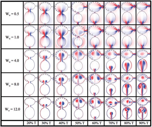
Vorticity analysis performed for the case of biologically sized trabeculae and varying |$Wo$| at different time points during one heart cycle.

Forces along the endocardial surface and trabeculae were calculated using the target point deformation force model, given by (8), and broken into the tangential and normal components. All forces are reported as dimensionless quantities.

It is clear from Fig. 6 that the region that experiences the largest force is on the left side of the ventricle, e.g. the side opposite to the bulbus arteriosus, when diastole finishes. Next we examined the the average magnitude of the force over a trabeculae over one heart cycle for |$Wo=0.8$|⁠, see Fig. 6b. During one heart beat, there appears to be three local extrema in the magnitude of the force for trabeculae |$\#3,\#4,\#5$|⁠, two local maxima and one local minimum. To decipher what forces were dominant, we computed the average magnitude of the normal and tangential components of the force on the trabeculae, as illustrated in Fig. 6c. The analysis shows that the normal component of the force dominates for trabeculae |$\#3,\#4,\#5$|⁠. Moreover, two local maxima and one local minimum are observed for the normal component of the force, averaged over the heartbeat. One local maximum appears for the tangential component of the force for |$Wo=0.8$|⁠.

Fig. 6.

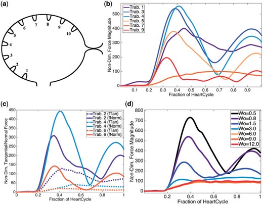
(a) Illustrating the indexing of trabeculae (b) Plot illustrating the average magnitude of the force on chosen trabeculae over the course of one heart cycle for |$Wo=0.8$|⁠, the biologically relevant case. (c) Plot showing the average magnitude of the tangential and normal forces at each time, for chosen trabeculae, during one heart cycle for |$Wo=0.8$|⁠. (d) A plot illustrating the average magnitude of force at each time-step for |$Wo$| ranging from |$0.5$| (half the biologically relevant case) to |$12.0$|⁠.

Furthermore, for trabecula |$\#3$|⁠, a scaling study was performed for |$Wo$| ranging from |$0.5$| to |$12.0$|⁠. Figure 6d depicts the average magnitude of the force over one heartbeat cycle for trabecula |$\#3$|⁠. The analysis yielded similar functional behaviour, compared with the analogous case in Fig. 6b, for |$Wo\leq3$|⁠. For |$Wo> 3$|⁠, there is a clear bifurcation where the average force magnitude no longer displays three local extrema, but instead appears to monotonically increase to an asymptotic maximum over one heartcycle.

3.1 Effects of trabeculae height

Figure 7 shows closed streamlines for |$Wo=\{0.5,1.0,4.0\}$| and trabecular heights ranging from half to twice the biologically relevant size. No blood cells were added to the simulations, and the trabeculae radii and locations were fixed, keeping them equidistant along the ventricular chamber. The analysis was performed within the ventricle immediately after diastole finishes, e.g. the ventricle stops expanding.

Fig. 7.

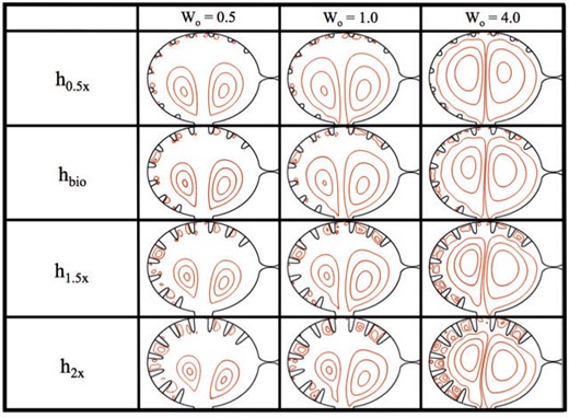
Streamline analysis for |$Wo=\{0.5,1.0,4.0\}$| and trabecular heights from half to twice the biologically relevant size. The analysis was performed within the ventricle immediately after diastole finishes and when the ventricle stops expanding.

In the |$h_{0.5x}$| case, i.e. half the biologically relevant height, some small vortices appear to form between trabeculae, as seen by the closed streamlines. These closed loops are small relative to the intertrabecular spacing. Note also that the flow velocities between the trabeculae are also quite small, see Fig. 8, which illustrates the magnitude of velocity for simulations of varying |$Wo$| for biologically relevant trabeculae heights. Large intracardial vortices are clearly present in all cases, and the size and strength of these vortices grow as |$Wo$| increases.

Fig. 8.

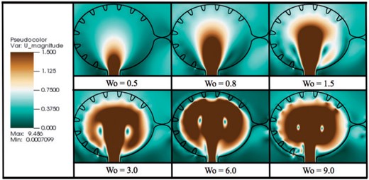
Magnitude of velocity colourmaps, corresponding to simulations of varying |$Wo$| for biologically relevant trabeculae height. The images were taken immediately after diastole, when the ventricle stops expanding.

As the trabeculae height increases, the intertrabecular vortices grow larger. The intracardial vortices remain approximately the same size as height increases. Note also that the intracardial vortex pair becomes more asymmetric as the trabeculae increase in height. Moreover, in the |$h_{1.5x}$| and |$h_{2x}$| cases, as |$Wo$| increases intertrabecular vortices become larger and increase in number (note that these regions still represented relatively slow flow).

The intracardial vortices both spin in opposite directions, e.g. the vortex to the left rotates counter-clockwise while the vortex on the right spins clockwise. Therefore, the intertrabecular vortices on the left side of the ventricle, which form near the head of the trabeculae, spin clockwise, and vice versa on the opposite side of the ventricle. Furthermore, there is a somewhat stagnant region opposite to the AV canal, where the two vortices diverge, and hence no large intertrabecular vortices form, as compared to different intertrabecular regions in the same simulation. There are small vortices that form in the intertrabecular region opposite to the AV canal in the |$h_{0.5x}$| cases; however, as the trabeculae increase in height in the |$Wo=0.5$| and |$Wo=1.0$| cases, this region becomes scarce of vortical flow, while there remains a small amount in the |$Wo=4.0$| case.

3.2 Effects of hematocrit

Figure 9 shows the effect that the addition of blood cells has in flow patterns over a range of |$Wo$|⁠. In these simulations, trabeculae height, radii, and spacing were fixed. Trabeculae heights were modelled at the biologically relevant size. The analysis was performed within the ventricle immediately at the completion of diastole.

Fig. 9.

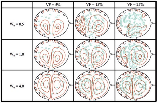
Streamline analysis for |$Wo=\{0.5,1.0,4.0\}$| and hematocrit of |$VF= \{5\%,15\%,25\%\}$|⁠. The analysis was performed within the ventricle immediately after diastole finishes and the ventricle ceases its expansion.

In the case of |$Wo=0.5$|⁠, it is clear the addition of blood cells alters the flow pattern within the ventricle. When |$VF=5\%$|⁠, the flow resembles that of the analogous case with no hematocrit as seen in Fig. 7; however, as hematocrit is increased to |$VF=15\%$|⁠, the flow patterns are very different. For |$VF=5\%, 15\%$|⁠, there are still coherent right or clockwise rotating vortices (shown as the closed streamlines) that form on the right side of the ventricle. The right vortex stretches directly above the AV canal and the left vortex is reduced. For |$VF = 25\%$|⁠, coherent intracardial vortices are not evident. For larger |$Wo$| (⁠|$Wo=1, 4)$|⁠, the coherent intracardial vortex pair is observed even for higher hematocrit.

In general as |$Wo$| increases, the intracardial vortices become more well-defined, e.g. vortical flow is smoother. However, in all cases hematocrit still affects vortical flow patterns intracardially as well as intertrabecularly. Moreover, in these simulations it is clear that after diastole, no blood cells have moved between trabeculae, but rather stay within the middle of the chamber, regardless of volume fraction of |$Wo$|⁠. These results suggest that for larger adult vertebrates, when the relative size of the blood cells would also be smaller, the presence of blood cells does not dramatically change the bulk flow. The blood cells do appear to affect the formation of coherent intracardial vortices at this stage of development when |$Wo = 0.5-1$|⁠.

3.3 Fluid mixing

As a rough approximation of the rotation and mixing in the fluid, we calculated that spatially-averaged vorticity in the ventricle. Figure 10 (a,b) give the spatially-averaged fluid vorticity on the left and right side of the ventricle, respectively, immediately after diastole, as a function of |$Wo$| for |$VF=\{0\%,5\%,\ldots,25\%\}$|⁠. It is evident that there is a non-linear relationship between spatially-averaged vorticity and |$Wo$|⁠. Furthermore, the overall net sign of the spatially-averaged vorticity is positive in the left side of the ventricle, while it is opposite on the right side. Moreover, the presence of blood cells does not appear to significantly affect the spatially-averaged fluid vorticity for |$Wo\leq1$|⁠, although it does affect the generation of a coherent vortex pair. %However, the effect of hematocrit may not be apparent at this snapshot in the heart cycle and more significant deviations between all cases may be seen at other times.

Fig. 10.

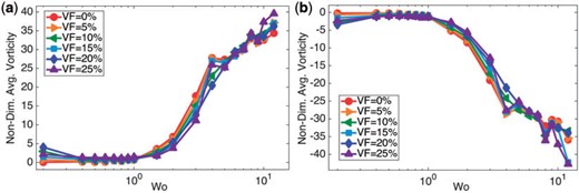
(a, b) Illustrate the average fluid vorticity on the left and right side of the ventricle, respectively, immediately after diastole, as a function of |$Wo$|⁠. It is clear there is a non-linear relationship between the spatially-averaged vorticity and biological scale, given by |$Wo$|⁠.

We report the spatially-averaged vorticity at different times during an entire heartbeat in each side of the ventricle in Fig. 11. The spatially averaged vorticity was calculated for |$Wo=\{0.5,0.8,1.5,8.0\}$| (note the biologically relevant case is |$Wo=0.8$|⁠) for hematocrit, |$VF=\{0\%,5\%,15\%,25\%\}$|⁠. When |$Wo\leq 1.5$|⁠, there is a clear peak before diastole ends (the vertical dotted line), while for |$Wo=8.0$|⁠, the peak occurs the moment when diastole ends. Note also that the width of this peak is larger for |$Wo=8.0$| when inertia dominates.

Fig. 11.

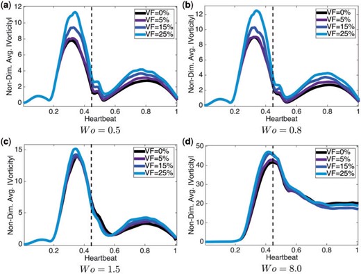
Plots of the spatially-averaged magnitude of vorticity for |$Wo=\{0.5,0.8,1.5,8.0\}$| for |$VF=\{0\%,5\%,15\%,25\%\}$|⁠. The vertical dotted line indicates when diastole ends. For every case of |$Wo$|⁠, the higher the hematocrit, the more spatially-averaged vorticity magnitude is induced.

In general as hematocrit increases, so does the spatially-averaged vorticity. Locally, the presence of blood cells act to increase vorticity in either direction through their tumbling motion, and this enhancement is not captured in the spatial average.

Although all Eulerian variables are initialized at zero, the resulting flow fields are not suspected to dramatically change between the first and subsequent heart cycles in the biologically relevant |$Wo$| regime. This is due to the high relative viscosity. For cases with |$Wo>1$|⁠, the flow fields in subsequent cycles may differ; however, as Figs 5, 7, 9, 10 and 11 illustrate, there is not much difference in the dynamics between the lower |$Wo\leq1$| cases. Note that in Fig. 9, the streamline analysis shows large differences between the |$Wo=0.5$| and |$Wo=1$| cases; however, the location of the blood cells are almost equivalent. The reason for the difference in streamlines is due to low velocities in the |$Wo=0.5$| case. Furthermore, the explicit streamlines in Fig. 9 are sensitive due to initial placement of the blood cells; however, the reason for the analysis is to highlight that there is different net fluid dynamic effects due to the addition of blood cells in cardiac models in heart development, more than the exact streamlines observed.

4. Conclusions

Two-dimensional immersed boundary simulations were used to solve for the fluid motion within an idealized two-chambered pumping heart. The presence of blood cells, trabeculae, and the relative importance of unsteady effects (e.g. the |$Wo$|⁠) were considered. The geometry models an idealized embryonic zebrafish heart at |$4\ \rm dpf$|⁠, and the motion of the chambers was approximated from the kinematic analysis of video taken from a wild type embryonic zebrafish. The main results of the study are as follows: (1) without the presence of blood cells, a large vortex pair forms in the ventricle during filling; (2) with the presence of blood cells at lower |$Wo$|⁠, a coherent vortex pair is not formed; (3) for |$Wo>4$|⁠, intertrabecular vortices form and vorticity separates from the trabeculae (suggesting the effect of the trabeculae is different in adult vertebrates than in embryos); (4) the presence of blood cells enhances spatially averaged vorticity in the ventricle, which peaks during diastole; (5) the presence of blood cells does not significantly alter the forces felt by the endocardial cells and (6) the majority of force is felt by the trabeculae on the outer region of the ventricle.

As mentioned above, an oppositely spinning large intracardial vortex pair forms for all |$Wo$| considered, here for |$Wo>0.2$|⁠. The vortex on the left spins counterclockwise, while the vortex on the right spins clockwise. This distinction becomes important when considering the formation of vortices between trabeculae. Larger intertrabecular vortices form for simulations with taller trabeculae. Furthermore, when the trabeculae height was |$1.5x$| or |$2x$| the biologically relevant height in the |$Wo=4$| case, stacked vortices formed between trabeculae; the top vortex spinning opposite to that of the closest intracardial vortex, while the vortex near the base spinning opposite to that. With the addition of blood cells, coherent intracardial vortices do not form when |$Wo<4$| and |$VF\leq15\%$|⁠; however, intertrabecular vortical flow patterns were not significantly changed as blood cells were not advected into these regions.

Note that the presence or absence of vortices alter the magnitude and direction of flow near the endocardial wall as well as the mixing patterns within the ventricle. When an intracardial vortex forms, the direction of the flow changes. The presence of two large intracardial vortices forms a stagnation point on the opposite side of the ventricle to the AV canal. Also, the presence of intertrabecular vortices changes the direction of the flow between trabeculae; not all intertrabecular regions have the formation of these vortices. In such cases, the direction of flow between different trabeculae will move in different directions. Since endothelial cells are known to sense and respond to changes in both magnitude and direction of flow (Heuslein et al., 2014), the formation and motion of intracardial and intertrabecular vortices may be important epigenetic signals.

For the biologically relevant parameter choices, |$Wo$| between |$0.5$| and |$1.0$|⁠, it is clear that the addition of blood cells significantly affects the formation of coherent vortices. This illustrates the importance of considering hematocrit when conducting fluid dynamics studies at this stage of development. Furthermore, this study demonstrates that small changes in viscosity, scale, morphology and hematocrit can influence bulk flow properties in the embryonic heart. This presents an interesting challenge since each of these parameters are continuously changing during heart morphogenesis. In addition, estimating the effective viscosity and hematocrit of the embryonic blood is nontrivial.

Moreover, 2D simulations are used as there is no highly resolved data available of the 3D morphology of the trabeculae at this developmental stage. As compared to adult mammalian cardiac trabeculae, the trabeculae in zebrafish at this stage are more bump-like, rather than elongated hoops. At biologically relevant |$Wo$| of these embryonic hearts, the importance of the 3D geometry for vortex shedding and vortex stretching will be minimum. We present a first step approach to the modelling of trabeculae, in which, future 3D studies can use as a basis of comparison. Furthermore, the benefits of 2D model make it feasible for large parameter sweeps, e.g. |$Wo$| sweeps, hematocrit sweeps, and trabeculae morphology sweeps, that 3D simulations would not allow for computational efficiency.

The results of this article demonstrate the importance of scale, morphology and the presence of blood cells in determining the bulk flow patterns through the developing heart. This is important because there is a strongly coupled relationship between intracardial haemodynamics, genetic regulatory networks, and cardiac conduction (Hu & Clarke, 1989; Hove et al., 2003; Bartman et al., 2004; Scherz et al., 2008; Culver & Dickinson, 2010; Santhanakrishnan & Miller, 2011; Garita et al., 2011; Granados-Rivero & Brook, 2012; Jamison et al., 2013; Chen et al., 2014; Samsa et al., 2015). Besides contractions of the myocardial cells, which in turn drive blood flow, haemodynamics are directly involved in proper pacemaker and cardiac conduction tissue formation (Tucker et al., 1988). Moreover, shear stress is found to regulate spatially dependent conduction velocities within the myocardium (Reckova et al., 2003). Myocardial contractions are also required for trabeculation (Samsa et al., 2015). It is important to note that changes in the conduction properties of the embryonic heart will also affect the intracardial shear stresses and pressures and patterns of cyclic strains.

The cyclic stresses and strains of the cardiomyocytes can also help shape the overall architecture of the trabeculated ventricle. The dynamics of these strains depend upon the intracardial fluid dynamics. For example, greater resistant to flow will induce larger cyclic stresses and possibly reduced cyclic strains. It is known that cyclic strains initiate myogenesis in the cellular components of primitive trabeculae (Garita et al., 2011). Since trabeculation first occurs near peak stress sites in the ventricle, altering blood flow may directly produce structural and morphological abnormalities in cardiogenesis. Previous work focusing on haemodynamic unloading in an embryonic heart has resulted in disorganized trabeculation and arrested growth of trabeculae (Bartman et al., 2004; Sankova et al., 2010; Peshkovsky et al., 2011). On the other hand, embryos with a hypertrabeculated ventricle also experience impaired cardiac function (Peshkovsky et al., 2011)

The exact mechanisms of mechanotransduction are not yet clearly understood (Weinbaum et al., 2003; Paluch et al., 2015). Biochemical signals are thought to be propagated throughout a pipeline of epigenetic signaling mechanisms, which may lead to a regulation of gene expression, cellular differentiation, proliferation, and migration (Chen et al., 2014). In vitro studies have discovered that endothelial cells can detect shear stresses as low as |$0.2\ \rm dyn/cm^2$| (Olesen et al., 1988) resulting in up or down regulation of gene expressions. Embryonic zebrafish hearts around |$36$| hpf are believed to undergo shear stresses of |$\sim$| 2 |$\rm dyn/cm^2$| and shear stresses of |$\sim$| 75 |$\rm dyn/cm^2$| by |$4.5$| dpf (Hove et al., 2003). Shear stresses in the |$\sim$|8–15 |$\rm dyn/cm^2$| range are known to cause cytoskeletal rearrangement (Davies et al., 1986). Mapping out the connection between fluid dynamics, the resulting forces, and the mechanical regulation of developmental regulatory networks will be critical for a global understanding of the process of heart development.

Acknowledgements

The authors would like to thank Steven Vogel for conversations on scaling in various hearts. We would also like to thank Lindsay Waldrop, Austin Baird, Leigh Ann Samsa, Julia Samson, William Kier and Arvind Santhanakrishnan for discussions on embryonic hearts.

Funding

This project was funded by NSF DMS CAREER #1151478, NSF CBET #1511427, NSF DMS #1151478 and NSF POLS #1505061 awarded to L.A.M. Funding for N.A.B. was provided from an National Institutes of Health T32 grant [HL069768-14; PI, Christopher Mack].