Aggregation and travelling wave dynamics in a two-population model of cancer cell growth and invasion

Abstract

Cells adhere to each other and to the extracellular matrix (ECM) through protein molecules on the surface of the cells. The breaking and forming of adhesive bonds, a process critical in cancer invasion and metastasis, can be influenced by the mutation of cancer cells. In this paper, we develop a nonlocal mathematical model describing cancer cell invasion and movement as a result of integrin-controlled cell–cell adhesion and cell–matrix adhesion, for two cancer cell populations with different levels of mutation. The partial differential equations for cell dynamics are coupled with ordinary differential equations describing the ECM degradation and the production and decay of integrins. We use this model to investigate the role of cancer mutation on the possibility of cancer clonal competition with alternating dominance, or even competitive exclusion (phenomena observed experimentally). We discuss different possible cell aggregation patterns, as well as travelling wave patterns. In regard to the travelling waves, we investigate the effect of cancer mutation rate on the speed of cancer invasion.

cancer mutation, two-population mathematical model, cell–cell and cell–matrix adhesion, integrins, aggregation patterns, travelling wave patterns

1. Introduction

Normal cells proliferate, divide and die in a highly controlled manner. This proliferation requires mitogenic signals, which are transmitted into the cell by the transmembrane receptors and bind signalling molecules, i.e. diffusible growth factors, extracellular matrix (ECM) components and cell–cell adhesion molecules (Hanahan & Weinberg, 2000). When a cell divides, its DNA is copied by the two new cells. However, if the DNA is damaged or not copied correctly, the new damaged cells will either die or start to proliferate in an uncontrolled manner, creating a signalling of oncogenes that act by mimicking growth signalling (Hanahan & Weinberg, 2000), eventually leading to an abnormal mass of tissues from cells that differ in clinically important phenotypic features (Marusyk et al., 2012). More precisely, tumour formation is a result of clonal expansion driven by somatic mutation, developed by a single precursor (monoclonal) that undergoes genetic and biological changes (Khalique et al., 2007; Nowell, 1976). This transformation of normal cells to cancer cells is a multistep process described via the steps of hyperplasia, premalignant change and dysplasia (Beckmann et al., 1997). Cancer cells lose their ability to regulate genome stability which leads to further genetic changes and tumour development (Khalique et al., 2007). Over the last three decades it has been shown experimentally that tumours consist of heterogeneous populations of cells, which are the result of genetic instability (Stackpole, 1983; Khalique et al., 2007; Loeb & Loeb, 2000; Martelotto et al., 2014). Intra-tumour heterogeneity appears in almost all phenotypic cell features: from cell morphology, to gene expression, motility, proliferation, immunogenicity and metastatic potential (Nicholson, 1984, 1987; Marusyk & Polyak, 2010). It should be mentioned that also normal cells are heterogeneous for various characteristics (e.g. surface antigens). Nevertheless, cellular heterogeneity is more pronounced in malignant neoplasms (Nicholson, 1987). Since the characteristics of the most abundant cell types inside these heterogeneous tumours might not necessarily predict the properties of mixed populations (Marusyk et al., 2012), we need to gain a better understanding of the dynamics of tumours formed of different mutated cell types. In fact, experimental studies have shown complex interactions between clonal sub-populations: from stable coexistence to dominant behaviours (Schuh et al., 2012). For example, some studies have shown the possibility of having competitive exclusion of clonal cancer cell sub-populations in heterogeneous tumours (Leith et al., 1989; Schuh et al., 2012). Other studies have shown that some tumour clones can compete with alternating dominance (Keats et al., 2012). We emphasize that the clonal composition of heterogeneous tumours usually changes over time (Greaves & Maley, 2012), and hence we can expect to see different competition outcomes as time increases (e.g. from transient coexistence of multiple clones to long-term competitive exclusion). Moreover, in some cancer clones there is evidence of contact domination, i.e. the inhibition of growth in some clones is the result of cell–cell contact between various cell sub-populations (Aabo et al., 1994).

The metastatic and invasive potential of heterogeneous tumours is influenced by the interactions amongst cells, and the interactions between cells and the ECM, via cell surface receptors and various cytokines and chemokines. A major group of cell surface receptors is represented by the integrins, which are involved in both cell–cell adhesion and cell–matrix adhesion (Weitzman et al., 1995). In particular, the successful colonization of new sites by cancer cells requires changes in integrin expression (Hanahan & Weinberg, 2000). Another group of molecules involved in cell–cell adhesion is represented by the cadherin families (Hanahan & Weinberg, 2000). The processes through which cells bind to each other and to ECM via these surface receptors, are responsible for tissue formation, stability and breakdown (Armstrong et al., 2006). In particular, to detach from the main aggregation/tissue, cells loose cell–cell adhesion and strengthen cell–matrix adhesion, which leads to ECM remodelling and degradation (with the help of enzymes called matrix metalloproteinases), thus helping cell migration through the ECM (Friedl & Wolf, 2003).

Over the last 20 years, mathematical models have been used intensively to try to gain a better understanding regarding the mechanisms behind cancer invasion and metastasis or the mechanisms behind the aggregation of other types of cells (see, e.g. Ambrosi & Preziosi (2002); Andasari & Chaplain (2012); Andasari et al. (2011); Anderson et al. (2000); Armstrong et al. (2006); Byrne & Preziosi (2003); Chaplain et al. (2011); Cristini et al. (2009); Deakin & Chaplain (2013); Domschke et al. (2014); Dyson et al. (2016); Enderling et al. (2006, 2010); Gerisch & Chaplain (2008); Green et al. (2010); Knútsdóttir et al. (2014); Mogilner & Edelstein-Keshet (1995); Mogilner et al. (1996); Painter et al. (2010); Sherratt et al. (2009); Painter et al. (2015) and many references therein). The early mathematical models were described by local systems of partial differential equations incorporating some generic chemotaxis or haptotaxis mechanisms (Gerisch & Chaplain, 2008; Painter, 2009), or incorporating implicit cell–cell interactions via tumour surface forces (Byrne & Chaplain, 1996). For example, Anderson et al. (2000) developed a local Partial Differential Equations (PDE) model of parabolic type for the invasion of cancer cells via cell–matrix interactions that lead to ECM degradation. Byrne & Chaplain (1996) modelled phenomenologically the influence of cell adhesion on tumour growth, by considering surface forces on tumour spheroids. As it became more clear that the movement in response to chemical/haptotactic gradients was facilitated by the binding and unbinding of cell surface molecules to other cells and to ECM, new mathematical models of parabolic type have been derived to describe these cell–cell and cell–matrix adhesion processes (Armstrong et al., 2006; Dyson et al., 2016; Gerisch & Chaplain, 2008; Gerisch & Painter, 2010; Green et al., 2010; Painter et al., 2015). Since these models incorporate the assumption that cells at position x bind/unbind to/from other cells at position x ± s (for some s > 0 within cells sensing radius), they are generally nonlocal. For example, Armstrong et al. (2006) focused on cell movements due to cell–cell adhesion, and introduced a nonlocal term that described the nature, the direction, as well as the strength of the adhesive forces between cancer cells. The authors also extended the nonlocal model to two populations that interact via adhesive forces (thus incorporating self-population and cross-population adhesion), and studied the effect of different adhesion strengths on the sorting or the mixing of cell populations. A similar two-population nonlocal model of parabolic type, which incorporated also cell proliferation and cell movement in response to cell ‘packing’, was described and investigated by Painter et al. (2015). The model in Armstrong et al. (2006) was further generalized by Gerisch & Chaplain (2008), Painter et al. (2010), Domschke et al. (2014) to include also cell-matrix interactions. While the majority of these models investigated cell–cell and cell–matrix adhesion in one cell population, a few models considered also multiple interacting cell populations (Domschke et al., 2014). In particular, Domschke et al. (2014) also assumed mutation between different cell populations. A different class of nonlocal models for cancer invasion has been developed in the context of the velocity-jump framework introduced in Othmer et al. (1988) and the kinetic models for active particles framework described, e.g. in Bellomo et al. (2010); see the transport models in Kelkel & Surulescu (2012), Lorenz & Surulescu (2014), Engwer et al. (2015, 2017), Hunt & Surulescu (2017).

We should emphasize here that all these nonlocal models for cell invasion are variations or generalizations of nonlocal models developed over the last two decades to describe the dynamics of cell populations (Edelstein-Keshet & Ermentrout, 1990), bacterial populations (Othmer et al., 1988; Xue et al., 2011; Perthame et al., 2016) or the dynamics of self-organized animal populations (Mogilner & Edelstein-Keshet, 1999; Topaz et al., 2006; Eftimie et al., 2007; Fetecau & Eftimie, 2010; Carrillo de la Plata et al., 2015; Fetecau, 2011). While the models describing collective cell movement are usually of parabolic type, the latest models for collective bacterial movement and collective animal movement are usually of hyperbolic/transport type.

In this study, we will investigate the role of cancer mutation on the possibility of clonal competition with alternating dominance or even competitive exclusion between two cancer cell sub-populations (as discussed before, these types of competition have been observed experimentally (Leith et al., 1989; Keats et al., 2012; Schuh et al., 2012)). To this end, we will introduce a nonlocal model for cell–cell and cell–matrix adhesion for two populations of cells (this model is a generalization of the models in Armstrong et al. (2006); Gerisch & Chaplain (2008); Painter et al. (2015)). However, in contrast to these previous models which are of parabolic type, here we consider a parabolic–hyperbolic model. More precisely, we assume that one ‘normal’ cancer cell population moves both randomly and in a directed manner in response to cell–cell and cell–matrix adhesive forces, while a second ‘mutant’ cancer cell population (i.e. a mutated clone) moves predominantly in a directed manner following cell–cell interactions (with cells from both populations) and cell–matrix interactions (as suggested by experimental observations in Goswami et al. (2005); Hagemann et al. (2005)). By incorporating this assumption, we aim to bring a more realistic approach to the models since the various intra-tumour cell sub-populations have been shown to be distinct not only in their adhesion capabilities but also in their motility and metastatic potential (Marusyk & Polyak, 2010). Moreover, we are interested in investigating the effect of mutation on the spreading speed of the mutated cancer cells, since the invasion levels of the mutant cancer cells are higher compared to those of ‘normal’ cancer cells (Chapman et al., 2014; Wojciechowska & Patton, 2015). Also, while previous nonlocal models have assumed constant adhesive interactions, here we will assume that these adhesive interactions depend on the level of integrins. Note that instead of assuming a kinetic (mesoscale) approach for cell-dependence on integrins as in Lorenz & Surulescu (2014), Engwer et al. (2015), Perthame et al. (2016), Engwer et al. (2017), Hunt & Surulescu (2017), here we follow a microscale–macroscale approach similar to Stinner et al. (2014, 2015, 2016) and Meral et al. (2015a,b) and couple the parabolic–hyperbolic model for spatial cell dynamics with an Ordinary Differential Equation (ODE) for integrins dynamics. We then investigate this complex multiscale model in terms of pattern formation, with particular attention being payed to the role of mutation rate on the coexistence (or not) of cell sub-populations that form stationary aggregations or travelling wave patterns.

The layout of this paper is as follows. In Section 2 we formulate a model of partial integro-differential equations for the dynamics of two cancer cell populations, coupled with ordinary differential equations describing ECM and integrins dynamics. In Section 3 we use linear stability analysis to investigate the ability of the model to form cell aggregations. In Section 4 we investigate numerically some types of spatio-temporal patterns exhibited by this nonlocal model. In Section 5 we investigate numerically and analytically travelling wave behaviours. We conclude in Section 6 with a summary and discussion of the results.

2. A mathematical model of two cancer cell sub-populations

2.1. Derivation of the model

Cancer invasion is a complex process involving cell–cell interactions, and interactions between cells and non-cellular components (Calvo & Sahai, 2011). To develop our model we consider two populations of cancer cells, a ‘normal’ (original clone) cancer population and a ‘mutant’ (descendant clone) population, which interact with each other as well as with the ECM via long-range adhesive and repulsive forces (Deman et al., 1976; Geiger, 1991); see Fig. 1.

Fig. 1.

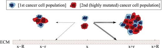
A caricature illustration of movement decisions made by cells at x, following interactions with neighbouring cells at x − r and x + r, and with the ECM. For very strong attraction (represented here by thicker arrows), cells move towards larger cell aggregations.

Let |$\varOmega \subset \mathbb {R}^{d} $| denote a bounded spatial domain (here we consider only d = 1; for a 2D version of the model see Appendix A), with periodic boundary conditions. Let |$I_{T} = \left [0,\infty \right )$| be the time interval. Denote by |$u_{1}\left (x,t\right )$| the density of ‘normal’ cancer cells at position x and time t, and by |$u_{2}\left (x,t\right )$| the density of ‘mutant’ cancer cells at position x and time t. We also denote by |$f\left (x, t\right )$| the ECM density, and by |$c\left (x, t\right )$| the density of integrin receptors on the surface of cancer cells (receptors involved in cell–cell and cell–matrix interactions). For compact notation, we define the vectors |$\underline {u}\left (x,t\right ) =\left ( u_{1}\left (x,t\right ), u_{2}\left (x,t\right )\right )^{\top }$| and |$\underline {\upsilon }\left (x,t\right ) =\left (\underline {u}\left (x,t\right ), f\left (x,t\right )\right )^{\top }$|⁠.

Dynamics of cancer cells. Experimental studies (Chapman et al., 2014) have shown that cancer cells can switch from a homogeneous type of invasion to a heterogeneous type of invasion described by invading chains (Chapman et al., 2014; Friedl & Wolf, 2003; Wojciechowska & Patton, 2015). Here, we assume that u₁ cells can mutate into u₂ cells at a constant rate M. We can derive a model for heterogeneous cancer cell populations by considering the equations

\begin{align} \frac{\partial u_{i}}{\partial t}=-\frac{\partial J_{i}}{\partial {x}}+(-1)^{i}Mu_{1}+G_{i}\left(\underline{u}\right),\quad i=1, 2, \end{align}

(2.1)

where J_i, i = 1, 2, are the cell fluxes and |$G_{i}\left (\underline {u}\right ), i=1, 2$|⁠, are the growth functions of populations u_i, i = 1, 2. The fluxes describe the factors that define cell movement. In this study we assume that the movement of the ‘normal’ cancer cell population u₁ is governed by random motility (which underlines a homogeneous type of invasion), as well as directed motility in response to cell–cell and cell–matrix adhesive forces (which underlines the heterogeneous type of invasion) (Calvo & Sahai, 2011). In contrast, the ‘mutant’ u₂ cell population moves only in a directed manner (hence exhibiting an heterogeneous type of invasion) in response to cell–cell and cell–matrix adhesion forces. Biologically, this directed movement of ‘mutant’ (more invasive) cancer cells can be explained by the increase of macrophage density near highly mutated cancer cells (Lin et al., 2006), which promotes the directed movement and invasion of these cancer cells, and decreases their random movement (Goswami et al., 2005; Hagemann et al., 2005). Therefore, in this study we assume that the movement of u₂ population due to random walk can be considered negligible. In this case, the total fluxes will be

\begin{align} J_{1}=J_{D}+J_{a_{1}} \;\; \text{and}\;\; J_{2}=J_{a_{2}}, \end{align}

(2.2)

where J_D is the flux due to Fickian diffusion, given by J_D = −D∂u₁/∂x, with D to be the diffusion coefficient, and |$J_{a_{i}}, \; i=1, 2$|⁠, are the adhesive fluxes for cell–cell and cell–matrix adhesion. In the case of u₂ the diffusion is considered very small and thus we ignore it.

Cell–cell/cell–matrix adhesion–mediated directed cancer cell migration occurs as a result of the social forces, i.e. attraction and repulsion, between cells and between cells and ECM components, when adhesive bonds are formed and broken. Cell–cell adhesion is described as the adhesion between cells of the same population, as well as cross-adhesion between cells of the two sub-populations. The cell–cell/cell–matrix adhesion forces are created through the binding of adhesion molecules, e.g. integrins, at cell surface. To model these forces, let us define R > 0 to be the sensing radius of the cells, i.e. the maximum range over which cells can detect other surrounding cells, which biologically represent the extent of the cell protrusions (e.g. filopodia) (Armstrong et al., 2006). Let |$g_{i}\left (\underline {\upsilon }\left (x+r, t\right ), c\left (x, t\right )\right ) i=1, 2$|⁠, describe the nature of the cell–cell and cell–matrix adhesive forces created at x due to signalling with cell/ECM components at x + r. These functions increase when the cell density and ECM density increase, and accordingly they decrease when the cell density and ECM density decrease. The functions g_i, i = 1, 2, are chosen as in Bitsouni et al. (2017) to be given by

\begin{align} g_{1}\left(\underline{\upsilon}\left(x+r, t\right), c\left(x, t\right)\right):=S_{1}\left(c\left(x, t\right)\right)u_{1}\left(x+r, t\right)+S\left(c\left(x, t\right)\right)u_{2}\left(x+r, t\right)+C_{1}\left(c\left(x, t\right)\right)f\left(x+r, t\right), \end{align}

(2.3)

and

\begin{align} g_{2}\left(\underline{\upsilon}\left(x+r, t\right), c\left(x, t\right)\right):=S_{2}\left(c\left(x, t\right)\right)u_{2}\left(x+r, t\right)+S\left(c\left(x, t\right)\right)u_{1}\left(x+r, t\right)+C_{2}\left(c\left(x, t\right)\right)f \left(x+r, t\right), \end{align}

(2.4)

where |$S_{i}\left (c\left (x, t\right )\right )$| is the cell–cell self-adhesion strength function for populations u_i, |$S\left (c\left (x, t\right )\right )$| is the cell–cell cross-adhesion strength function between the two populations, and |$C_{i}\left (c\left (x, t\right )\right )$| is the adhesion strength function between population u_i and ECM. We should mention here that a similar term was considered before by Chaplain et al. (2011). Other studies (Armstrong et al., 2006; Gerisch & Chaplain, 2008) consider volume filling effect to avoid unbounded aggregations. While unbounded aggregations are possible in this type of nonlocal models, these have not been observed in our system (at least not for the parameter ranges used in this study).

We define these adhesion strength functions in terms of the integrin density c: the more integrins a cell has, the stronger its adhesion force (Gallant et al., 2005). However, the adhesion strength reaches a plateau for a large integrin density (Maheshwari et al., 2000). Thus, we require an increasing, bounded function, so that we avoid extreme phenomena for large values of integrin density. A biologically realistic choice is a sigmoid function. This choice is supported by various other experimental studies in the literature which have shown that different biological processes can be described by sigmoid functions: from cell adhesion via integrins (Cutler & García, 2003; Michael et al., 2009), to oxygen saturation (Shiao & Ou, 2007). Note also that since cell mutation could lead to more integrins (Kidera et al., 2010), we consider strength functions with different integrin levels for each of the two populations. To this end, we choose the adhesion strength functions to be given by:

\begin{align} S_{1}\left(c\right)&={s_{1}}^{\ast}\left(1+\tanh\left(a_{1} c\right)\right),\; S_{2}\left(c\right)={s_{2}}^{\ast}\left(1+\tanh\left(a_{2} c\right)\right),\; S\left(c\right)=s^{\ast}\left(1+\tanh\left(dc\right)\right), \nonumber\\ C_{1}\left(c\right)&={c_{1}}^{\ast}\left(1+\tanh\left(b_{1} c\right)\right),\; C_{2}\left(c\right)={c_{2}}^{\ast}\left(1+\tanh\left(b_{2} c\right)\right), \end{align}

(2.5)

where d, a_i, b_i, i = 1, 2, and s*, s_i*, c_i*, i = 1, 2, are positive real numbers.

Within this sensing radius, let us now define K_cc and K_cm, the kernels for cell–cell and cell–matrix adhesion ranges, respectively:

\begin{align*} K_{cc}\left(r\right)= \left[\begin{array}{@{}cc@{}} K_{11}\left(r\right) & K_{12}\left(r\right)\\ K_{21}\left(r\right) & K_{22}\left(r\right) \end{array}\right],\quad K_{cm}\left(r\right)= \left[\!\!\begin{array}{cc} K_{1}\left(r\right) \\ K_{2}\left(r\right) \end{array}\!\!\right]. \end{align*}

These interaction kernels describe the dependency of the force magnitude on the distance r from x. Here K_ij, i, j = 1, 2, are the interaction kernels between population i and population j (i.e. cell–cell interactions), and K_i, i = 1, 2, are the kernels for cell–matrix interactions (for the two populations). For simplicity, throughout this study we will consider (see also Domschke et al., 2014):

\begin{align} K_{11}=K_{12}=K_{1}\ \text{and}\ K_{22}=K_{21}=K_{2}. \end{align}

(2.6)

Moreover, we assume that these kernels are attractive at medium/long ranges (i.e. at the edges of the cell) and repulsive at very short ranges (i.e. over cell surface), and thus can be defined as

\begin{align} K_{1,2}(r):=q_{a}K^{1,2}_{a}(r)-q_{r}K^{1,2}_{r}(r), \end{align}

(2.7)

with q_a and q_r describing the magnitudes of attractive and repulsive interactions, and |$K_{a}^{1,2}(r)$| and |$K_{r}^{1,2}(r)$| describing the spatial ranges over which these interactions take place. We will discuss various examples of attractive (K_a) and repulsive (K_r) kernels in Section 3, in the context of linear stability analysis.

Therefore, the local cell–cell and cell–matrix adhesion forces will be described by the product of functions g_i and |$K_{i}\left (r\right ),\; i=1, 2$|⁠. To describe the nonlocal cell–cell and cell–matrix adhesion and repulsion forces (Deman et al., 1976; Geiger, 1991), we sum all such forces by integrating over space to obtain the total forces:

\begin{align} F_{1}[{\kern.6pt}\underline{u}, f, c](x,t)&:=\frac{1}{R}{\int_{0}^{R}}\sum_{k=0}^{1} \eta(k) K_{1}(r)g_{1}(\underline{\upsilon}(x+r\eta(k), t), c(x, t))\ \mathrm{d}r, \end{align}

(2.8)

and

\begin{align} F_{2}[{\kern.6pt}\underline{u}, f, c](x,t)&:=\frac{1}{R}{\int_{0}^{R}}\sum_{k=0}^{1} \eta(k) K_{2}(r)g_{2}(\underline{\upsilon}(x+r\eta(k), t), c(x, t))\, \mathrm{d}r, \end{align}

(2.9)

where |$\eta \left (k\right )=\left (-1\right )^{k}, k=0, 1$|⁠, is the direction of the forces. Thus, the full nonlocal interaction terms are described by

\begin{align} F_{1}[{\kern.6pt}\underline{u}, f,c](x,t)=&\frac{1}{R}{\int_{0}^{R}} \sum_{k=0}^{1} \eta(k) K_{1}(r)\big[S_{1} (c)u_{1}(x+r\eta(k),t)+S(c) u_{2}(x+r\eta(k),t)\big]\ \mathrm{d}r\nonumber\\ &+\frac{1}{R}{\int_{0}^{R}} \sum_{k=0}^{1} \eta(k) K_{1}(r)C_{1}(c)f(x+r\eta(k),t)\ \mathrm{d}r, \end{align}

(2.10)

and

\begin{align} F_{2}[{\kern.6pt}\underline{u}, f,c](x,t)=&\frac{1}{R}{\int_{0}^{R}} \sum_{k=0}^{1} \eta(k) K_{2}(r)\big[S_{2} (c)u_{2}(x+r\eta(k),t)+S(c) u_{1}(x+r\eta(k),t)\big]\ \mathrm{d}r\nonumber\\ &+\frac{1}{R}{\int_{0}^{R}} \sum_{k=0}^{1} \eta(k) K_{2}(r)C_{2}(c)f(x+r\eta(k),t)\ \mathrm{d}r. \end{align}

(2.11)

We assume that the adhesive fluxes are proportional to the density of the cells and the nonlocal adhesion forces, F_i, i = 1, 2. Thus, we obtain the following expressions for the two adhesive fluxes:

\begin{align} J_{a_{i}}=u_{i}F_{i}[{\kern.6pt}\underline{u}, f, c], \quad i=1, 2. \end{align}

(2.12)

Substituting (2.12) into the general mass conservation equations, we have the following equations describing the dynamics of the two cancer cell populations:

\begin{align} \frac{\partial u_{1}}{\partial t}=D\frac{\partial^{2} u_{1}}{\partial x^{2}} -\frac{\partial}{\partial x} \left(u_{1}F_{1}[{\kern.6pt}\underline{u}, f, c]\right)-Mu_{1}+G_{1}(\underline{u}), \end{align}

(2.13a)

\begin{align} \frac{\partial u_{2}}{\partial t}=-\frac{\partial}{\partial x} \left(u_{2}F_{2}[{\kern.6pt}\underline{u}, f, c]\right)+Mu_{1}+G_{2}(\underline{u}). \end{align}

(2.13b)

We assume that both u₁ and u₂ cells can proliferate in a logistic manner (to describe the observed slow-down in tumour growth following the loss of nutrients (Laird, 1964)). Thus, the growth functions are given by

\begin{align} G_{i}(\underline{u})=r_{i}u_{i}\left(1-\frac{u_{1}+u_{2}}{k_{u}}\right)\!,\quad i=1,2, \end{align}

(2.14)

where r₁ and r₂ are the growth rates of the u₁ and u₂ populations, respectively, and k_u is the carrying capacity. Note that these growth functions incorporate also the principle of competition between clonal sub-populations in heterogeneous tumours (Leith et al., 1989).

ECM dynamics. Cancer cell populations degrade the ECM upon contact. Moreover, ECM density is remodelled back to normal levels by cancer and healthy cells. Thus, the dynamics of ECM, f(x, t), can be described by:

\begin{align} \frac{\partial f}{\partial t}=-\alpha u_{1}{\kern2pt}f-\beta u_{2}{\kern2pt}f+\gamma\left(1-\frac{u_{1}+u_{2}}{k_{u}}-\frac{f}{f_{m}}\right), \end{align}

(2.15)

where α and β are the positive rate constants of ECM degradation by u₁ and u₂ cell populations, respectively, k_u is the carrying capacity of the cancer cell populations and f_m is the maximum ECM density at which the ECM fills up all available physical space. Following the approach of Anderson et al. (2000); Gerisch & Chaplain (2008), we choose to ignore the ECM remodelling terms for this model, i.e. we always use γ = 0.

Integrin dynamics. We assume that the level of integrins depends on cancer cell density. Moreover, we assume that cell mutation changes the density of receptors (since in highly metastatic cancers, the expression of integrins is up-regulated (Kidera et al., 2010)). We follow an approach similar to (Stinner et al., 2014, 2015, 2016; Meral et al., 2015a,b) and assume that the dynamics of integrins c(x, t) can be described by an ODE:

\begin{align} \frac{\partial c}{\partial t}=p_{1}u_{1}+p_{2}u_{2}-qc, \end{align}

(2.16)

where q is the decay rate of c, and p₁ and p₂ are the production rates of integrins by population u₁ and u₂, respectively. To model the increase in receptors on mutant cancer cells, we assume that p₂ > p₁ (see Table 2). Note that integrins are produced at the positions where these cells exist, and as cells move to different spatial positions the integrins will be produced at these new positions, too (this can be seen more clearly in Figs 4–10). Moreover, the production of integrins at various positions in space is counterbalanced by the decay term (−qc), which ensures that integrins will be removed from regions where cells do not exist.

For the initial conditions, we start with only population |$u_{1}\left (x,0\right )={u_{1}^{0}}\left (x\right )$|⁠. The second population u₂, arises from mutations in the population u₁ after a period of time, and thus |$u_{2}\left (x,0\right )=0.$| For the ECM, we assume that the tumour has already degraded some of its surrounding tissues:

\begin{align} f(x,0)=1-0.5u_{1}(x,0)-0.5u_{2}(x,0). \end{align}

(2.17)

Finally, the integrin density, c, is proportional to the initial tumour cell density

\begin{align} c(x,0)=0.5u_{1}(x,0)+0.5u_{2}(x,0). \end{align}

(2.18)

To complete our model we need to impose boundary conditions. Throughout this study we assume that the two cancer cell populations move on a circular finite domain of length L, i.e. |$x\in \left [0, L\right ]$|⁠. The periodic boundary conditions that model this movement are

\begin{align} u_{1}(0, t)=u_{1}(L, t)\ \text{and}\ u_{2}(0, t)=u_{2}(L, t). \end{align}

(2.19)

Note that with this choice of boundary condition, the nonlocal terms are wrapped around the domain. We will return to this aspect in Section 4.

 

Remark 2.1

Note that equations (2.13)–(2.16) describe a ‘microscale–macroscale’ model, where the spatially-averaged microscale integrin dynamics (described by an ODE) is coupled with the spatial dynamics of cancer cells (described by nonlocal PDEs). As mentioned above, this modelling approach follows various other recent studies on cancer cell–matrix adhesion via integrins (Stinner et al., 2014, 2015, 2016; Meral et al., 2015a,b). Moreover, the coupling of PDEs for cell movement with ODEs for the dynamics of cell receptors has been considered not only for cancer cells but also for other types of cells, such as ‘Dictyostelium’ cells (Höfer et al., 1995a,b). However, the past 10–15 years have seen the development of structured cell population models (described by ‘mesoscale’ models) where the macroscopic cell dynamics is dependent on a microscopic variable that characterizes the cells at molecular level (Erban & Othmer, 2004, 2005; Xue et al., 2011; Lorenz & Surulescu, 2014; Engwer et al., 2015; Perthame et al., 2016; Engwer et al., 2017; Hunt & Surulescu, 2017). In Appendix B we present a modified mesoscale version of model (2.13)–(2.16) where we assume that the two cancer cell populations are structured by an internal variable that describes the integrin level. (Here we use the terminology of ‘mesoscale’ and ‘microscale–macroscale’ models in the same spirit as Stinner et al. (2014), Lorenz & Surulescu (2014) and Hunt & Surulescu (2017).)

2.2. Non-dimensionalization of the model

To non-dimensionalize system (2.13) and equations (2.15)–(2.16), we define the following quantities:

\begin{align} \tilde{t}&=\frac{t}{\tau}, \tilde{x}=\frac{x}{L_{0}}, \tilde{u}_{1}=\frac{u_{1}}{k_{u}}, \tilde{u}_{2}=\frac{u_{2}}{k_{u}}, \tilde{f}=\frac{f}{f_{m}}, \tilde{c}=\frac{c}{c_{m}}, \tilde{R}=\frac{R}{L_{0}}, \tilde{r}=\frac{r}{L_{0}},\nonumber\\\tilde{S}\left(\tilde{c}\right) &=\frac{\tau k_{u}}{{L_{0}^{2}}}S\left(c_{m}\tilde{c}\right), \tilde{S_{i}}\left(\tilde{c}\right)=\frac{\tau k_{u}}{{L_{0}^{2}}}S_{i}\left(c_{m}\tilde{c}\right), \tilde{C_{i}}\left(\tilde{c}\right)=\frac{\tau f_{m}}{{L_{0}^{2}}}C_{i}\left(c_{m}\tilde{c}\right), i=1, 2. \end{align}

(2.20)

Here, L₀ is a length scale, defined as the maximum invasion distance of the cancer cells at the ‘normal’ of invasion (Anderson et al., 2000). Usually L₀ is in the range of 0.1–1 cm. We rescale time with |$\tau :={L_{0}^{2}}/D_{\tau }$|⁠, where D_τ is the characteristic diffusion coefficient (∼ 10⁻⁶cm²s⁻¹). In addition, we rescale the cancer cells, the ECM and the integrins with k_u, f_m and c_m, respectively. Here k_u is the carrying capacity of the cancer cell populations and it is taken to be ∼ 6.7 ⋅ 10⁷cell/volume, and f_m is the maximum ECM density at which the ECM fills up all available physical space and it is taken to be equal to 4 mg/volume, as in Domschke et al. (2014). Finally, c_m is the maximum integrin density and it is taken to be 5 ⋅ 10⁴ integrins per cell (as in Benedetto et al. (2006)). For the kernels |$K_{i}\left (r\right ), i=1,2, $| we choose (as in Domschke et al. (2014)) the dimensionless functions |$\tilde {K_{i}}\left (\tilde {r}\right ), i=1,2, $| given by

\begin{align*} \tilde{K_{i}}\left(\tilde{r}\right):=L_{0}K_{i}\left(L_{0}\tilde{r}\right)=L_{0}K_{i}\left(r\right),\quad i=1, 2. \end{align*}

We define the dimensionless functions |$\tilde {g_{i}} (\tilde {\underline {u}}, \tilde {f}, \tilde {c} ), i=1, 2$|⁠, by

\begin{align*} \tilde{g_{i}}\left(\tilde{\underline{u}}, \tilde{f}, \tilde{c}\right):=\frac{\tau}{{L_{0}^{2}}}g_{i}\left(\underline{u}, f, c\right),\quad i=1, 2. \end{align*}

Therefore, we have for the nonlocal terms |$F_{i}[\kern2pt\underline {u}, f, c], i=1, 2$|⁠, that

\begin{align*} \tilde{F_{i}}\left[\tilde{\underline{u}}, \tilde{f}, \tilde{c}\right]:=\frac{\tau}{L_{0}}F_{i}\left[{\kern.6pt}\underline{u}, f, c\right], i=1, 2. \end{align*}

Finally, we obtain the dimensionless parameters:

\begin{align} \tilde{D}=\frac{D}{D_{\tau}}, \;\tilde{M}=\tau M, \;\tilde{\alpha}=\tau\alpha k_{u}, \;\tilde{\beta}=\tau\beta k_{u}, \;\tilde{q}=\tau q, \;\tilde{r_{i}}=\tau r_{i}, \;\tilde{p_{i}}=\frac{\tau p_{i}k_{u}}{c_{m}},\; i=1,2. \end{align}

(2.21)

After dropping the tildes for notational convenience, we obtain the following non-dimensionalized system

\begin{align} \frac{\partial u_{1}}{\partial t}=D\frac{\partial^{2} u_{1}}{\partial x^{2}}-\frac{\partial}{\partial x} \left(u_{1}F_{1}\left[{\kern.6pt}\underline{u}, f, c\right]\right)-Mu_{1}+r_{1}u_{1}\left(1-u_{1}-u_{2}\right), \end{align}

(2.22a)

\begin{align} \frac{\partial u_{2}}{\partial t}=-\frac{\partial}{\partial x} \left(u_{2}F_{2}\left[{\kern.6pt}\underline{u}, f, c\right]\right)+Mu_{1}+r_{2}u_{2}\left(1-u_{1}-u_{2}\right), \end{align}

(2.22b)

\begin{align} \frac{\partial f}{\partial t}=-\alpha u_{1}{\kern2pt}f-\beta u_{2}{\kern2pt}f, \end{align}

(2.22c)

\begin{align} \frac{\partial c}{\partial t}=p_{1}u_{1}+p_{2}u_{2}-qc. \end{align}

(2.22d)

From now on, we will always refer to the non-dimensional quantities. In the next two sections, we discuss the dynamics of model (2.22).

3. Linear stability analysis of the model

Next, we investigate the conditions under which the two populations of cancer cells form aggregations. We first calculate the spatially homogeneous steady states of the model, and then apply standard linear stability analysis to investigate the conditions (for parameter values) under which the two cancer cell populations can form aggregations.

To start, we look for the homogeneous steady states of the ODE model associated to system (2.22), that describes the growth and mutation of the two cancer cell populations and the temporal dynamics of ECM and integrins (i.e. no spatial movement):

\begin{align} \frac{\partial u_{1}}{\partial t}=-Mu_{1}+r_{1}u_{1}\left(1-u_{1}-u_{2}\right)=0, \end{align}

(3.1a)

\begin{align} \frac{\partial u_{2}}{\partial t}=Mu_{1}+r_{2}u_{2}\left(1-u_{1}-u_{2}\right)=0, \end{align}

(3.1b)

\begin{align} \frac{\partial f}{\partial t}=-\alpha u_{1}{\kern2pt}f-\beta u_{2}{\kern2pt}f=0, \end{align}

(3.1c)

\begin{align} \frac{\partial c}{\partial t}=p_{1}u_{1}+p_{2}u_{2}-qc=0, \end{align}

(3.1d)

which has the following steady state solutions |$\left (u_{1}^{\ast }, u_{2}^{\ast }, f^{\ast }, c^{\ast }\right ):$|

\begin{align} \left(0, 0, f^{\ast}, 0\right) \; \text{and}\; \left(0, 1, 0, \frac{p_{2}}{q}\right), \end{align}

(3.2)

with |$f^{\ast }\geqslant 0$|⁠. Here we consider only the non-negative solutions, since we require biological realism. Note that all these homogeneous steady states have u₁ = 0 (so the more invasive population u₂ persists longer). However, as we will see in Section 4, the model can exhibit non-homogeneous steady states with u₁(x, t) ≠ 0.

We now investigate the stability of the steady states for the spatially homogeneous and spatially heterogeneous systems, to see if the introduction of spatial dynamics (i.e. cell movement and cell–cell/cell–matrix adhesion) can lead to instabilities. First, we substitute the steady states (3.2) into the Jacobian matrix of the spatially homogeneous system (3.1) and calculate the four eigenvalues corresponding to each steady state. Thus, for the steady state |$\left (0, 0, f^{\ast }, 0\right )$| we have the eigenvalues

\begin{align} \lambda_{1}=0,\quad \lambda_{2}=-M+r_{1},\quad \lambda_{3}=r_{2}>0\ \text{and}\ \lambda_{4}=-q<0. \end{align}

(3.3)

Since λ₃ > 0, this state is unstable. For the steady state |$\left (0, 1, 0, p_{2}/q\right )$| we obtain the eigenvalues

\begin{align} \lambda_{1}=-\beta <0,\quad \lambda_{2}=-M<0,\quad \lambda_{3}=-r_{2}<0\ \text{and}\ \lambda_{4}=-q<0. \end{align}

(3.4)

Since all eigenvalues are negative, the state (0, 1, 0, p₂/q) is always linearly stable to homogeneous perturbations.

Next, we investigate the linear stability analysis of the spatial system (2.22). To this end, we apply small spatial perturbations to the previous homogeneous steady states: |$u_{i}(x,t)=u_{i}^{\ast }+\bar {u}_{i}(x,t), i=1, 2, f(x,t)=f^{\ast }+\bar {f}(x,t),\; c(x,t)=c^{\ast }+\bar {c}(x,t)$|⁠, where |$\bar {u}_{1}, \bar {u}_{2}, \bar {f}$| and |$\bar {c}$| denote the small perturbations. (Note that, to avoid negative solutions when we perturb the zero steady states, we consider |$\bar {u}_{1}\left (x,t\right ), \bar {u}_{2}\left (x,t\right ), \bar {f}\left (x,t\right ),\bar {c}\left (x,t\right )\geqslant 0$|⁠.) Substituting these into the system (2.22) (after the adhesion strength functions S_i(c), S(c), C_i(c), i = 1, 2, have been expanded in Taylor series), and ignoring non-linear terms, leads to the following linearized system:

\begin{align} \frac{\partial \bar{u}_{1}}{\partial t}=&\,D\frac{\partial^{2}\bar{u}_{1}}{\partial x^{2}}-\frac{u_{1}^{\ast}}{R}\frac{\partial}{\partial x}\left\lbrace{\int_{0}^{R}}K_{1}(r) S_{1}\left(c^{\ast}\right)\left(\bar{u}_{1}(x+r,t)-\bar{u}_{1}(x-r,t)\right)\ \mathrm{d}r\right\rbrace\nonumber\\[10pt] &-\frac{u_{1}^{\ast}}{R}\frac{\partial}{\partial x}\left\lbrace{\int_{0}^{R}}K_{1}(r)\left[S\left(c^{\ast}\right)\left(\bar{u}_{2}(x+r,t)-\bar{u}_{2}(x-r,t)\right)+C_{1}\left(c^{\ast}\right)\left(\,\bar{f}(x+r,t)-\bar{f}(x-r,t)\right)\right]\mathrm{d}r\right\rbrace\nonumber\\[10pt] &-M\bar{u}_{1}+r_{1}\bar{u}_{1}\left(1-2u_{1}^{\ast}-u_{2}^{\ast}\right)-r_{1}u_{1}^{\ast}\bar{u}_{2}, \end{align}

(3.5a)

\begin{align} \frac{\partial \bar{u}_{2}}{\partial t}=&-\!\frac{u_{2}^{\ast}}{R}\frac{\partial}{\partial x}\!\left\lbrace{\!\int_{0}^{R}}\!K_{2}(r)\left[S_{2}\left(c^{\ast}\right)\left(\bar{u}_{2}(x+r,t)-\bar{u}_{2}(x-r,t)\right)+S\left(c^{\ast}\right)\!\left(\bar{u}_{1}(x+r,t)-\bar{u}_{1}(x-r,t)\right)\right] \mathrm{d}r\right\rbrace\nonumber\\[10pt] &-\!\frac{u_{2}^{\ast}}{R}\frac{\partial}{\partial x}\!\left\lbrace{\int_{0}^{R}}\!K_{2}(r)C_{2}\left(c^{\ast}\right)\left({\kern1pt}\bar{f}(x+r,t)-\bar{f}(x-r,t)\right) \mathrm{d}r\right\rbrace\! +M\bar{u}_{1}+r_{2}\bar{u}_{2}\left(1-u_{1}^{\ast}-2u_{2}^{\ast}\right)\!-\!r_{2}u_{2}^{\ast}\bar{u}_{1}, \end{align}

(3.5b)

\begin{align} \frac{\partial \bar{f}}{\partial t}=-\alpha\left(\bar{u}_{1}{\kern2pt}f^{\ast}+u_{1}^{\ast}{\kern2pt}\bar{f}\right)-\beta \left(\bar{u}_{2}{\kern2pt}f^{\ast}+u_{2}^{\ast}{\kern2pt}\bar{f}\right), \end{align}

(3.5c)

\begin{align} \frac{\partial \bar{c}}{\partial t}=p_{1}\bar{u}_{1}+p_{2}\bar{u}_{2}-q\bar{c}. \end{align}

(3.5d)

We look for solutions of the form |$A_{u_{1}}e^{ikx+\lambda t},\; A_{u_{2}}e^{ikx+\lambda t},\; A_{f}e^{ikx+\lambda t}$| and A_ce^ikx+λt with |$\lvert A_{u_{1}}\rvert $|⁠, |$\lvert A_{u_{2}}\rvert $|⁠, |$\lvert A_{f}\rvert $|⁠, |$\lvert A_{c}\rvert \ll 1$|⁠, where k and λ are the wave number and frequency, respectively. Then system (3.5) reduces to

\begin{align} \lambda A_{u_{1}}=&-\!k^{2}D A_{u_{1}}+\frac{2ku_{1}^{\ast}}{R}\left[S_{1}\left(c^{\ast}\right)A_{u_{1}}+S\left(c^{\ast}\right)A_{u_{2}}+C_{1}\!\left(c^{\ast}\right)A_{f}\right]\hat{K}^{s}_{1}\left(k\right)-M A_{u_{1}}\!+r_{1}A_{u_{1}}\!\left(1-2u_{1}^{\ast}-u_{2}^{\ast}\right)\nonumber\\ &-r_{1}u_{1}^{\ast}A_{u_{2}}, \end{align}

(3.6a)

\begin{align} \lambda A_{u_{2}}=\frac{2ku_{2}^{\ast}}{R}\left[S_{2}\left(c^{\ast}\right)A_{u_{2}}+\!S\left(c^{\ast}\right)A_{u_{1}}\!+C_{2}\left(c^{\ast}\right)A_{f}\right]\hat{K}^{s}_{2}\left(k\right)+M A_{u_{1}}+r_{2}A_{u_{2}}\left(1-u_{1}^{\ast}-2u_{2}^{\ast}\right)-r_{2}u_{2}^{\ast}A_{u_{1}}, \end{align}

(3.6b)

\begin{align} \lambda A_{f}=-\alpha\left(A_{u_{1}}{\kern2pt}f^{\ast}+u_{1}^{\ast}A_{f}\right)-\beta \left(A_{u_{2}}{\kern2pt}f^{\ast}+u_{2}^{\ast}A_{f}\right), \end{align}

(3.6c)

\begin{align} \lambda A_{c}=\ p_{1}A_{u_{1}}\ +\ p_{2}A_{u_{2}}-\ qA_{c}, \end{align}

(3.6d)

where |$\hat {K}_{1,2}^{s}\left (k\right )={\int _{0}^{R}}K_{1,2}\left (r\right )\sin \left (kr\right )\ \mathrm {d}r$| are the Fourier sine transforms of the kernels |$K_{1,2}\left (r\right )$|⁠. For simplicity, throughout the rest of this study, we will assume that K₁(r) = K₂(r) =: K(r) and thus |$\hat {K}^{s}_{1}(k)=\hat {K}^{s}_{2}(k)=:\hat {K}^{s}(k)$|⁠.

Cellular aggregations form when the steady states |$(u_{1}^{*},u_{2}^{*},f^{*},c^{*})$| are unstable to spatial perturbations, and for this to happen we require the maximum real part of eigenvalues of the Jacobian matrix of system (3.6) to be positive, for at least one discrete value of k > 0.

• For the state |$\left (u_{1}^{\ast }, u_{2}^{\ast }, f^{\ast }, c^{\ast }\right )=\left (0, 0, f^{\ast }, 0\right )$| we obtain the eigenvalues

  \begin{align} \lambda_{1}=0, \;\;\; \lambda_{2}=-k^{2}D-M+r_{1}, \;\;\; \lambda_{3}=r_{2}>0, \;\;\; \lambda_{4}=-q<0. \end{align}

  (3.7)

  Thus, the steady state |$\left (u_{1}^{\ast }, u_{2}^{\ast }, f^{\ast }, c^{\ast }\right )=\left (0, 0, f^{\ast }, 0\right )$| is unstable.

• For the state |$\left (u_{1}^{\ast }, u_{2}^{\ast }, f^{\ast }, c^{\ast }\right )=\left (0, 1, 0, p_{2}/q\right )$| we obtain the eigenvalues

  \begin{align} \lambda_{1}=-\beta <0, \quad \lambda_{2}=-k^{2}D-M<0, \quad \lambda_{3}=S_{2}\left(c^{\ast}\right)Y\left(k\right)-r_{2}, \quad \lambda_{4}=-q<0, \end{align}

  (3.8)

  where |$Y\left (k\right )=\frac {2k}{R}\hat {K}^{s}\left (k\right )$|⁠. Recall that in the absence of diffusion and advection, the steady state |$\left (u_{1}^{\ast }, u_{2}^{\ast }, f^{\ast }, c^{\ast }\right )=\left (0, 1, 0, p_{2}/q\right )$| is linearly stable. Thus, for aggregation to form, we require this state to be unstable to spatially inhomogeneous perturbations (Benson et al., 1993), i.e. the maximum real part of the eigenvalues to be greater than zero. Since λ₁, λ₂, λ₄ < 0, the steady state |$\left (0, 1, 0, p_{2}/q\right )$| is unstable if the following dispersion relation holds:

  \begin{align} Re\left(\lambda_{3}\left(k\right)\right)=Re\left(-r_{2}+\frac{2ks^{\ast}_{2}}{R}\left(1+\tanh\left(a_{2}\frac{p_{2}}{q}\right)\right)\hat{K}^{s}\left(k\right)\right)>0. \end{align}

  (3.9)

We notice that this dispersion relation, and therefore the possibility of cell aggregations to form, depends on the choice of the interaction kernel. Mogilner & Edelstein-Keshet (1999) showed that the type of kernel affects the possibility of movement and/or aggregation. Throughout the rest of this study, we will consider translated Gaussian attraction and repulsion kernels (as in Eftimie et al. (2007); Carrillo de la Plata et al. (2015)):

\begin{align} K\left(x\right)=\frac{q_{a}}{\sqrt{2\pi {m^{2}_{a}}}}e^{-\frac{\left(x-s_{a}\right)^{2}}{2{m^{2}_{a}}}}-\frac{q_{r}}{\sqrt{2\pi {m^{2}_{r}}}}e^{-\frac{\left(x-s_{r}\right)^{2}}{2{m^{2}_{r}}}}, \end{align}

(3.10)

where s_a and s_r represent half of the length of attraction and repulsion ranges, respectively, with s_r < s_a. Also, m_j = s_j/8, j = a, r, represent the width of the attractive and the repulsive interaction ranges. (The constants m_j, j = a, r, are chosen such that the support of more than 98% of the mass of the kernels is inside the interval |$\left [0, \infty \right )$| (Eftimie et al., 2007).) In Section 3.1 we will investigate how different types of kernels lead to different dispersion relations.

The Fourier sine transform of kernel (3.10) is given by

\begin{align} \hat{K}^{s}\left(k\right)=\int_{-\infty}^{\infty}K\left(r\right)\sin\left(kr\right)\ \mathrm{d}r=q_{a}e^{-\frac{(km_{a})^{2}}{2}}\sin(ks_{a})-q_{r}e^{-\frac{(km_{r})^{2}}{2}}\sin(ks_{r}). \end{align}

(3.11)

Therefore, relation (3.9) becomes

\begin{align} -r_{2}+\frac{2ks^{\ast}_{2}}{R}\left(1+\tanh\left(a_{2}\frac{p_{2}}{q}\right)\right)\left(q_{a}e^{-\frac{(km_{a})^{2}}{2}}\sin(ks_{a})-q_{r}e^{-\frac{(km_{r})^{2}}{2}}\sin(ks_{r})\right)>0, \end{align}

(3.12)

where the imaginary part of the eigenvalue |$\lambda _{3}\left (k\right )$| will be zero.

An example of such dispersion relation is shown in Fig. 2. Note the steady-state/steady-state mode interaction that occurs when we increase the parameters q_a and q_r (i.e. the strength of attractive and repulsive cell–cell interactions). There is a range of k −values for which |$Re\left (\lambda _{3}\left (k\right )\right )$| is positive, and thus aggregations can arise from spatial perturbations of the steady state |$\left (u_{1}^{\ast }, u_{2}^{\ast }, f^{\ast }, c^{\ast }\right )=\left (0, 1, 0, p_{2}/q\right )$|⁠. This means that the steady state |$\left (0, 1, 0, p_{2}/q\right )$|⁠, which is linearly stable for the homogeneous system, is destabilized due to the spatial dynamics (diffusion and advection). Setting diffusion coefficient zero we observe that there is still a range of k −values for which |$Re\left (\lambda _{3}\left (k\right )\right )>0$|⁠, implying the adhesion-driven instability.

Fig. 2.

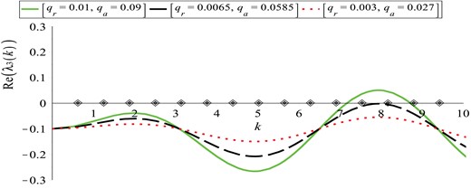
Plot of the dispersion relation (3.12) for the steady state |$\left (0, 1, 0, p_{2}/q\right )$|⁠. The curves represent Re(λ₃(k)) for: (a) q_r = 0.01, q_a = 0.09 (solid green curve); (b) q_r = 0.0065, q_a = 0.0585 (dashed black curve); (c) q_r = 0.003, q_a = 0.027 (dotted red curve); the rest of the model parameters are given in Table 2. The diamonds on the x-axis represent the discrete wave numbers |$k_{j}=2\pi j/L, j=1, 2, \dots $|⁠. The two critical wave numbers that become unstable at the same time (giving rise to steady-state/steady-state mode interactions) are k₁₂ and k₁₃.

 

Remark 3.1

Note that model (2.22) does not exhibit Hopf bifurcations (i.e. |$Re\left (\lambda \left (k\right )\right )=0, Im\left (\lambda \left (k\right )\right )\neq 0$|⁠). Therefore, although aggregations will develop, there will be no travelling patterns that arise via Hopf bifurcations.

3.1. Aggregation with different types of kernel

In Mogilner & Edelstein-Keshet (1999) it was shown that even kernels give rise to group drift, while odd kernels have a greater effect in regions where the distribution of the density is uneven (e.g. the edges of the population), leading to stationary groups. Considering the importance of the symmetry of the interaction kernels, we next discuss the cases of even and odd kernels, and compare these results with our previous results where we used a translated Gaussian kernel (see equation (3.10)), to investigate the possibility of cell aggregations to form from spatial perturbation of the steady state |$\left (u_{1}^{\ast }, u_{2}^{\ast }, f^{\ast }, c^{\ast }\right )=\left (0, 1, 0, p_{2}/q\right )$|⁠.

• Aggregation with even kernel

  We consider the situation that the interaction kernel is an even function with respect to the y-axis. We choose the following Gaussian kernel (Mogilner & Edelstein-Keshet, 1999):

  \begin{align} K\left(x\right):=\frac{q_{a}}{\sqrt{2\pi {m^{2}_{a}}}}\exp\left(-x^{2}/2{m^{2}_{a}}\right)-\frac{q_{r}}{\sqrt{2\pi {m^{2}_{r}}}}\exp\left(-x^{2}/2{m^{2}_{r}}\right), \end{align}

  (3.13)

  where q_a, q_r, m_a and m_r have the same meaning as in equation (3.10). The Fourier sine transform of the above even kernel is zero: |$\hat {K}^{s}\left (k\right )=0$|⁠. We know (see equation (3.8)) that the Jacobian matrix of system (3.6) has three negative eigenvalues λ_{1, 2, 4} < 0. For the even kernel considered here we also have

  \begin{align} \lambda_{3}\left(k\right)&=-r_{2}<0. \end{align}

  (3.14)

  Therefore, the steady state |$\left (u_{1}^{\ast }, u_{2}^{\ast }, f^{\ast }, c^{\ast }\right )=\left (0, 1, 0, p_{2}/q\right )$| is stable, and no aggregations will form.

• Aggregation with an odd kernel

  We investigate now the stability of |$\left (u_{1}^{\ast }, u_{2}^{\ast }, f^{\ast }, c^{\ast }\right )=\left (0, 1, 0, p_{2}/q\right )$| when we consider an odd kernel with respect to the origin. To this end, we choose

  \begin{align} K\left(x\right):=\frac{q_{a}x}{\sqrt{2\pi {m^{2}_{a}}}}\exp\left(-x^{2}/2{m^{2}_{a}}\right)-\frac{q_{r}x}{\sqrt{2\pi {m^{2}_{r}}}}\exp\left(-x^{2}/2{m^{2}_{r}}\right), \end{align}

  (3.15)

  where q_a, q_r, m_a and m_r have the same meaning as in equation (3.10). Then the Fourier sine transform of the kernel (3.15) is

  \begin{align} \hat{K}^{s}\left(k\right)=q_{a}k{m_{a}^{2}}{\exp}(-(km_{a})^{2}/2)-q_{r}k{m_{r}^{2}}{\exp}(-(km_{r})^{2}/2). \end{align}

  (3.16)
  As before, the Jacobian matrix of system (3.6) has three negative eigenvalues: λ_{1, 2, 4} < 0. The stability of the state |$\left (0, 1, 0, p_{2}/q\right )$| is given by the sign of

  \begin{align} Re\left(\lambda_{3}\left(k\right)\right)=-r_{2}+\frac{2k^{2}s^{\ast}_{2}}{R}\left(1+\tanh\left(a_{2}\frac{p_{2}}{q}\right)\right)\left(q_{a}{m_{a}^{2}}e^{-\frac{\left(km_{a}\right)^{2}}{2}}-q_{r}{m_{r}^{2}}e^{-\frac{\left(km_{r}\right)^{2}}{2}}\right). \end{align}

  (3.17)

  In Fig. 3 we plot |$Re(\lambda _{3}\left (k\right ))$| against the wave number k for this steady state. We observe that for values of q_a greater than those in the translated Gaussian case (see Fig. 2), there is a range of k–values for which |$Re\left (\lambda _{3}\left (k\right )\right )$| is positive, thus the steady state |$\left (0, 1, 0, p_{2}/q\right )$| can become unstable, and spatial aggregations could arise.

Fig. 3.

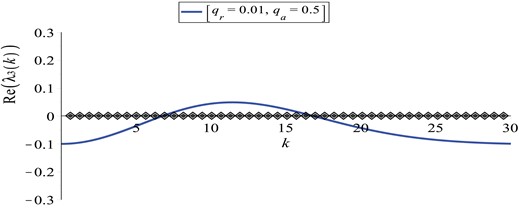
Plot of the dispersion relation (3.17) for the steady state |$\left (u_{1}^{\ast }, u_{2}^{\ast }, f^{\ast }, c^{\ast }\right )=\left (0, 1, 0, p_{2}/q\right )$|⁠. Here, q_a = 0.5. The rest of the model parameters are given in Table 2. The solid curve represents the real part of λ₃, while the diamonds represent the discrete wave numbers |$k_{j}=2\pi \frac {j}{L}, j=0, 1, 2, \dots $|⁠.

4. Numerical results

In this Section we investigate numerically the stability of model (2.22). To discretize our model we use a time-splitting approach. First, we use a Crank–Nicolson scheme to propagate the solution of the diffusion term. Then, we use the Nessyahu–Tadmor scheme (Nessyahu & Tadmor, 1990) for the time-propagation of the advection terms. Finally, for the time-propagation of the reaction terms we use a forth order Runge–Kutta algorithm, where the integrals are further discretized using the Simpson’s rule. All simulations are performed on a domain of length L = 10 with periodic boundary conditions, and for time up to t = 500. Because of the periodic boundary conditions, we wrap the integrals around the domain. The initial conditions for the cancer cell populations are either small random perturbations of spatially homogeneous steady states

\begin{align*} u_{i}(x,0)&=u_{i}^{*}+rand(0,10^{-4}), \quad i=1,2,\nonumber\\ f(x,0)&=f^{*}+rand(0,10^{-4}), \nonumber\\ c(x,0)&=c^{*}+rand(0,10^{-4}),\nonumber \end{align*}

or small random perturbations of rectangular-shaped aggregations located in the middle of the domain

\begin{align} u_{i}(x,0)= \begin{cases} {u_{i}^{c}}+rand(0,10^{-4}), & x\in(L/2-1,L/2+1) \\ 0, &\ \text{everywhere}\; \text{else} \end{cases} \end{align}

(4.1)

with |${u_{1}^{c}}=0$| and |${u_{2}^{c}}$| as specified in the caption of the figures. The initial conditions for the ECM and integrin density depend on cancer cell density, and are given by relations (2.17) and (2.18), for all numerical simulations.

Stationary aggregation patterns. To check the validity of our results obtained via linear stability analysis (see Fig. 2), we first run simulations for small random perturbations of the spatially homogeneous steady state |$\left (u^{\ast }_{1}, u^{\ast }_{2}, f^{\ast }, c^{\ast }\right )=(0, 1, 0, p_{2}/q)$|⁠, and for q_a = 0.09 and q_r = 0.01. The results, presented in Fig. 4, show 12–13 stationary pulses (corresponding to critical wave numbers k₁₂ − k₁₃). The spread of cancer cells over the whole domain (panels (a), (b)) leads to the degradation of ECM (panel (c)). The integrin density (panel (d)) follows the patterns in the density of cancer cells. We observe here a coexistence between a low u₁ population and a high u₂ population.

Fig. 4.

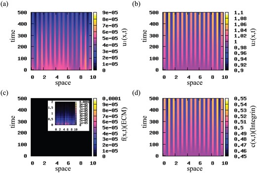
Patterns exhibited by model (2.22) for small random perturbations of the steady state |$\left (0, 1, 0, p_{2}/q\right )$|⁠, corresponding to the dispersion relation shown in Fig. 2. Here, we use the cell–cell interaction kernel given by relation (3.10), and the model parameters given in Table 2. (a) Density of u₁ cell population; (b) density of u₂ (highly mutated) cell population; (c) ECM density f; (d) integrin density c. Note the formation of 12 or 13 peaks (if counting separately the peaks on the periodic boundaries) of high cell density corresponding to critical wave numbers k₁₂/k₁₃.

To check the effect of initial data on model dynamics, in Fig. 5 we investigate the behaviour of model (2.22) when we change the initial conditions to a rectangular pulse describing an initial aggregation of tumour cells. The magnitudes of attractive-repulsive interactions (and all other parameter values) are the same as in Fig. 4. The short-term results in Fig. 5(a)–(d) show a travelling pulse behaviour exhibited by the u₂ population that moves away from population u₁ (which is mostly stationary—although even this population spreads a bit). This faster spreading of the u₂ cells compared to the u₁ cells is consistent with experimental observations (Chapman et al., 2014; Wojciechowska & Patton, 2015). The movement of u₂ population eventually stops near the boundary (due to the periodic boundary conditions, the left-moving and right-moving subgroups can sense each other across the boundary). The fast-moving u₂ cells degrade the ECM (panel (c)). We also note the high density of integrins associated with the u₁ population (panel (d)). The long-term results in Fig. 5(a^′)–(d^′) show the formation of new aggregations of cells at distant positions in space. For t ∈ (100, 250), the two tumour populations coexist. For t > 250, population u₁ is slowly eliminated and population u₂ dominates the dynamics of model (2.22). We also note that despite some chaotic-like dynamics exhibited by the u₁ and u₂ populations for t < 300, in the long term the system approaches stationary pulses defined by 13 peaks (corresponding to unstable wave number k₁₃).

Fig. 5.

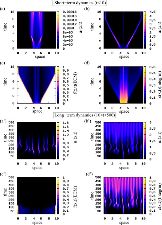
Short-term and long-term patterns exhibited by model (2.22). The initial conditions for the two cancer cell populations are described by a rectangular pulse (see (4.1)) with |${u_{2}^{c}}=1.0$|⁠. We use the interaction kernel given by (3.10), and the model parameters given in Table 2. (a),(a^′) Density of u₁ population; (b),(b’) density of u₂ (highly mutated) population; (c),(c^′) ECM density f; (d),(d^′) integrin density c.

In Figs 6 and 7 we investigate the effect of various mutation rates on the dynamics of the u₁ and u₂ populations. In Fig. 6 we choose M = 0.001 (see Table 2), and observe that population u₂ vanishes for t > 400, while population u₁ persists and forms small high-density aggregations of cells. This unexpected behaviour might be explained by the combined effect of three factors: (i) the mutation rate (M = 0.001) that is much smaller than the growth rates (r_{1, 2} = 0.1) of the two cancer cell populations, (ii) the lack of diffusion for u₂ and (iii) the competition for nutrients between the two cell populations (which is modelled implicitly by the logistic terms G_{1, 2}; see equations (2.14)). This eventually leads to an overall increase in the first population, u₁, and a decrease in the second (highly mutated) population, u₂. In Fig. 7 we increase the mutation rate to M = 0.05, while chosing the growth rates fixed at r₁ = r₂ = 0.1. We observe that faster mutation rates lead to a decrease and eventual elimination of the u₁ population. The u₂ population increases and dominates the long-term dynamics of model (2.22).

Fig. 6.

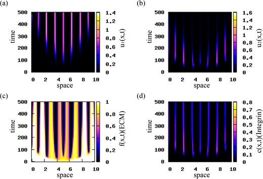
Patterns exhibited by model (2.22). The initial conditions for the cancer cell populations consist of a rectangular pulse (see (4.1)) with |${u_{2}^{c}}=0.001$|⁠. The mutation rate is M = 0.001. The rest of model parameters are given in Table 2. (a) Density of u₁ population; (b) density of u₂ population; (c) ECM density f; (d) integrin density c.

Fig. 7.

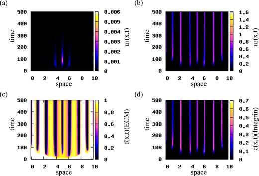
Patterns exhibited by model (2.22). The initial conditions for the cancer cell populations consist of a rectangular pulse (see (4.1)) with |${u_{2}^{c}}=0.001$|⁠. The mutation rate in M = 0.05. The rest of model parameters are given in Table 2. (a) Density of u₁ population; (b) density of u₂ population; (c) ECM density f; (d) integrin density c.

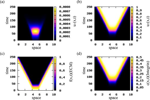
Travelling wave patterns. Choosing again rectangular pulse initial conditions, we reduce the magnitudes of cell–cell attractive and repulsive interactions to q_a = 0.00025 and q_r = 0.0005. The numerical simulations in Fig. 8 show travelling waves that propagate in opposite directions at a constant speed. Similar behaviour is obtained for q_a > q_r. The evolution of the travelling waves is shown in Fig. 9 for |$t=25j,\; j=1,\dots ,9$|⁠. We observe that the waves connect the unstable steady states |$\left (0, 1, 0, p_{2}/q\right )$|⁠, with p₂/q = 0.5, and |$\left (0, 0, f^{\ast }, 0\right )$|⁠, with f* = 1.

Fig. 8.

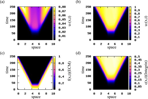
Patterns exhibited by model (2.22) for initial conditions for the two cancer cell populations consisting of a rectangular pulse with |${u_{2}^{c}}=0.001$|⁠. Here, q_r = 0.0005, q_a = 0.00025 and the rest of the model parameters are given in Table 2. (a) Cell density for u₁ population; (b) cell density for u₂ population; (c) ECM density f; (d) integrin density c. Travelling waves are obtained for the translated Gaussian kernel given by relation (3.10).

Fig. 9.

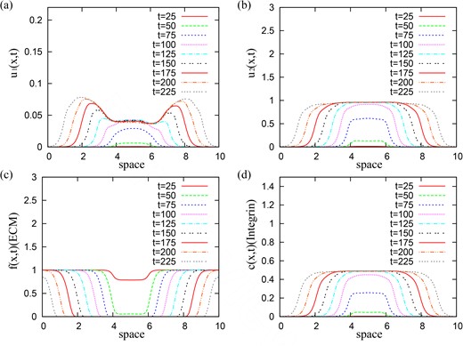
The evolution of the travelling waves under small perturbations for q_r = 0.0005, q_a = 0.00025 and the rest of the model parameters given in Table 2, of (a) cancer cell density u₁ of the first (‘normal’) population; (b) cancer cell density u₂ of the second (‘mutant’) population; (c) ECM density f; (d) integrin density c.

Finally, we check the effect that an increase in the mutation rate M has on the travelling wave behaviour exhibited by model (2.22). Figure 10 shows that for high mutation rates (M = 0.05) the first population still exhibits a travelling wave before vanishing.

 

Remark 4.1

To understand the long-term behaviour of model (2.22) with odd kernels, we also ran numerical simulations using the interaction kernel given by (3.15). The spatial patterns obtained in this case were similar to the patterns obtained for the translated Gaussian kernel (see relation (3.10)).

4.1. Summary of model variables and parameters

Here we present two tables with the model variables and parameters. In Table 1 we list the model variables with their units. In Table 2 we list the parameters of our model and their corresponding units and non-dimensional values used in the simulations.

Parameter estimation.

• For the diffusion coefficient, Chaplain & Lolas (2006) has shown a range between |$\tilde {D}= 10^{-5}$| and |$\tilde {D}=10^{-3}$|⁠. In this study, we choose |$\tilde {D}=10^{-4}$|⁠.

• The sensing radius was based on the range of values given in (Armstrong et al., 2006; Gerisch & Chaplain, 2008). In this study, we choose |$\tilde {R}=0.99$|⁠.

• Attraction and repulsion ranges were chosen to be smaller or equal to sensing radius, with the repulsion range to be smaller than the attraction range (Green et al., 2010).

• Various experimental studies (Cunningham & You, 2015; Morani et al., 2014) have shown that doubling times for tumour cells range from 1–10 days. This corresponds to growth rates between |$(\ln (2)/10, \ln (2)/1)=(0.07, 0.7)$|⁠. In this study, we assume that |$\tilde {r_{1}}=\tilde {r_{2}}=0.1$|⁠.

• Experimental studies (Cillo et al., 1987; Hill et al., 1984; Mareel et al., 1991) have shown that the mutation rate ranges between M = 10⁻³/day and M = 0.1/day. Thus the non-dimensional value of the mutation rate is in the range between |$\tilde {M}=0.001$| and |$\tilde {M}=0.1$| (for highly aggressive tumours). In this study, we choose |$\tilde {M}=0.001$|⁠.

• The parameters |$a_{i}, d, b_{i}, s_{i}^{\ast }, s^{\ast }, c_{i}^{\ast }, i=1, 2$|⁠, were based on the range of the adhesion strength parameters used in Armstrong et al. (2006).

• Experimental studies (Kidera et al., 2010) have shown greater production of integrins for highly mutated cancer cells. Thus, we choose |$\tilde {p_{1}}<\tilde {p_{2}}$|⁠.

• Experimental studies (Delcommenne & Streuli, 1995; Davis et al., 2001; Liu et al., 2011; Lobert et al., 2010) have shown that the half-lifes of the integrins range from 0.04–4 days. This corresponds to decay rate between |$\left (\ln \left (2\right )/4, \ln \left (2\right )/0.04\right )=\left (0.17, 17.3\right )$|⁠. In this study, we assume that |$\tilde {q}=0.2$|⁠.

Fig. 10.

Patterns exhibited by model (2.22) for higher mutation rates (M = 0.05) and initial conditions for the two cancer cell populations consisting of a rectangular pulse with |${u_{2}^{c}}=0.001$|⁠. Here, q_r = 0.0005, q_a = 0.00025 and the rest of the model parameters are given in Table 2. (a) Cell density for u₁ population; (b) cell density for u₂ population; (c) ECM density f; (d) integrin density c. Travelling waves are obtained for the translated Gaussian kernel given by relation (3.10)

5. Speed of travelling waves

The numerical simulations showed that the model exhibits travelling wave solutions (see Figs 8 and 9). In this section we estimate the minimum speed at which these waves could propagate (assuming that the travelling waves do exist). We assume that close to the invading front, the nonlinear differential equations describing the spread of a population have similar speeds as their linear approximation (see the approaches in Medlock & Kot (2003); Mollison (1991)). Therefore, we first calculate the linearized system (3.5) at the steady state |$\left (u_{1}^{\ast }, u_{2}^{\ast }, f^{\ast }, c^{\ast }\right )=\left (0, 1, 0, p_{2}/q\right )$|⁠. In travelling wave coordinates z = x − wt (where |$u_{i}\left (x,t\right )=U_{i}\left (z\right ), i=1, 2,\; f\left (x,t\right )=F\left (z\right ),\; c\left (x,t\right )=C\left (z\right )$|⁠), this system becomes:

\begin{align} -wU^{\prime}_{1}\left(z\right)=DU^{\prime\prime}_{1}\left(z\right)-MU_{1}\left(z\right), \end{align}

(5.1a)

\begin{align} -wU^{\prime}_{2}\left(z\right)=&-\frac{1}{R}\frac{\partial}{\partial z}\left\{\int_{0}^{R}K(r)\left[S_{2}(p_{2}/q)(U_{2}(z+r)-U_{2}(z-r))+\right.\right.\nonumber\\& \left.\left.\phantom{\int_{0}^{R}K(r)}+S(p_{2}/q)(U_{1}(z+r)-U_{1}(z-r))+C_{2}(p_{2}/q)(F(z+r)-F(z-r))\right]\ \mathrm{d}r\right\}\nonumber\\ &+MU_{1}\left(z\right)-r_{2}\left(U_{1}\left(z\right)+U_{2}\left(z\right)\right), \end{align}

(5.1b)

\begin{align} -wF^{\prime}\left(z\right)=-\beta F\left(z\right), \end{align}

(5.1c)

\begin{align} -wC^{\prime}\left(z\right)=p_{1}U_{1}\left(z\right)+p_{2}U_{2}\left(z\right)-qC\left(z\right). \end{align}

(5.1d)

Let s₁, s₂, s₃, s₄ > 0 be the steepness (i.e. exponent of an exponential decay/increase profile) of u₁, u₂, f, c. The minimum of |$w\left (s_{j}\right )$| for |$s_{j}>0, \; j=1,\dots ,4$|⁠, gives an upper bound on the rightward travelling wave speed of the nonlinear system. Thus, we make the general exponential ansatz

Table 1

A list of model variables with their units. Since we are in 1D, length and volume coincide and we express the variables in terms of domain length.

Variable	Description	Dimensional Units
u1	‘Normal’ cancer cell density	cell/length
u2	‘Mutant’ cancer cell density	cell/length
f	ECM density	mg/length
c	Integrin density	integrins/cell

Table 2

A list of model parameters with their units and their non-dimensional values, obtained from (2.20) and (2.21), which we used during numerical simulations.

Param.	Description	Dimensional Units	Non-dim. value (⁠|$\tilde {p}$|⁠)	Reference
D	Diffusion coefficient	length2/time	10−4	Chaplain & Lolas (2006)
R	Sensing radius	length	0.99	Armstrong et al. (2006)
qa	Magnitude of attraction	length2/cell	0.09	Estimated
qr	Magnitude of repulsion	length2/cell	0.01	Estimated
sa	Attraction range	length	0.99	Estimated
sr	Repulsion range	length	0.25	Estimated
ma	Width of attraction kernel	length	0.99/8	Estimated
mr	Width of repulsion kernel	length	0.25/8	Estimated
r1	Growth rate of u1	1/time	0.1	Cunningham & You (2015); Morani et al. (2014)
r2	Growth rate of u2	1/time	0.1	Cunningham & You (2015); Morani et al. (2014)
M	Mutation rate	1/time	0.001	Cillo et al. (1987); Hill et al. (1984); Mareel et al. (1991)
a1	Coeff. related to the number of integrins necessary for max self-adhesion between u1	cell/integrins	0.3	Estimated
a2	Coeff. related to the number of integrins necessary for max self-adhesion between u2	cell/integrins	0.01	Estimated
d	Coeff. related to the number of integrins necessary for max cross-adhesion	cell/integrins	0.5	Estimated
b1	Coeff. related to the number of integrins necessary for max cell-ECM adhesion for u1	cell/integrins	1.8	Estimated
b2	Coeff. related to the number of integrins necessary for max cell-ECM adhesion for u2	cell/integrins	5	Estimated
|$s^{\ast }_{1}$|	Magnitude of self-adhesion forces of u1	|$length/\left (time\cdot \textit {cell}\right )$|	0.9	Estimated
|$s^{\ast }_{2}$|	Magnitude of self-adhesion forces of u2	|$length/\left (time\cdot \textit {cell}\right )$|	0.2	Estimated
s*	Magnitude of cross-adhesion forces	|$length/\left (time\cdot \textit {cell}\right )$|	1	Estimated
				(continued).

Table 2

Continued.

Param.	Description	Dimensional Units	Non-dim. value (⁠|$\tilde {p}$|⁠)	Reference
|$c^{\ast }_{1}$|	Magnitude of cell-ECM forces of u1	|$length/\left (time\cdot \textit {cell}\right )$|	1.5	Estimated
|$c^{\ast }_{2}$|	Magnitude of cell-ECM forces of u2	|$length/\left (time\cdot \textit {cell}\right )$|	5.5	Estimated
α	Rate of ECM degradation by u1	|$length/\left (time\cdot \textit {cell}\right )$|	1	Sherratt et al. (2009)
β	Rate of ECM degradation by u2	|$length/\left (time\cdot \textit {cell}\right )$|	2	Sherratt et al. (2009)
p1	Production rate of c by u1	|$integrins/\left (time\cdot \textit {cell}\right )$|	0.05	Estimated
p2	Production rate of c by u2	|$integrins/\left (time\cdot \textit {cell}\right )$|	0.1	Estimated
q	Decay rate of c	1/time	0.2	Liu et al. (2011)

\begin{align} U_{1}\left(z\right)=A_{1}e^{-s_{1}z},\; U_{2}\left(z\right)=A_{2}e^{-s_{2}z},\; F\left(z\right)=A_{3}e^{s_{3}z}\ \text{and}\ C\left(z\right)=A_{4}e^{-s_{4}z}, \end{align}

(5.2)

where |$A_{j}\in \mathbb {R}, j=1,\dots , 4$|⁠, such that asymptotically we have |$U_{i}\left (z\right )\to 0, i=1, 2,\; F\left (z\right )\to f^{\ast },\; C\left (z\right )\to 0$| as |$z\to +\infty $|⁠. First we investigate the |$s_{j}, \; j=1,\dots ,4$|⁠, numerically. In Fig. 11 we fit these exponential ansatz profiles (given by (5.2)) to the numerical solutions u₁(x, t), u₂(x, t), f(x, t) and c(x, t) at time t = 175 (dotted curve). We obtain the following ansatz profiles (continuous curve in Fig. 11):

Fig. 11.

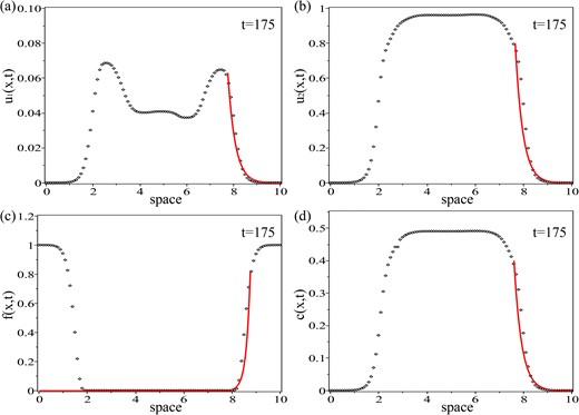
Plot of the numerical simulations of the travelling wave profile, shown in Figs 8 and 9, for (a) population u₁ and the exponential ansatz function |$E_{1}\left (x\right )$| given by relation (5.3) with |$A_{1}=0.063\cdot \exp \left (24.5675\right )$|⁠; (b) population u₂ and the exponential ansatz function |$E_{2}\left (x\right )$| given by relation (5.4) with |$A_{2}=0.8\cdot \exp \left (24.2505\right )$|⁠; (c) ECM density, f, and the exponential ansatz function |$E_{3}\left (x\right )$| given by relation (5.5) with |$A_{3}=0.82\cdot \exp \left (-52.5\right )$|⁠; (d) integrin density, c, and the exponential ansatz function |$E_{4}\left (x\right )$| given by relation (5.6) with |$A_{4}=0.4\cdot \exp \left (24.092\right )$|⁠. Here, q_r = 0.0005, q_a = 0.00025 and the rest of the model parameters are given in Table 2.

\begin{align} E_{1}\left(x\right)=A_{1}\cdot \exp\left(-3.17x\right),\ \ \text{with}\ A_{1}=0.063\cdot\exp\left(24.5675\right), \end{align}

(5.3)

\begin{align} E_{2}\left(x\right)=A_{2}\cdot \exp\left(-3.17x\right),\ \ \text{with}\ A_{2}=0.8\cdot\exp\left(24.2505\right), \end{align}

(5.4)

\begin{align} E_{3}\left(x\right)=A_{3}\cdot \exp\left(6x\right),\ \ \text{with}\ A_{3}=0.82\cdot\exp\left(-52.5\right), \end{align}

(5.5)

\begin{align} E_{4}\left(x\right)=A_{4}\cdot \exp\left(-3.17x\right),\ \ \text{with}\ A_{4}=0.4\cdot\exp\left(24.092\right). \end{align}

(5.6)

Hence, we deduce that the travelling wave profiles of |$U_{1}\left (z\right ), U_{2}\left (z\right )$| and |$C\left (z\right )$| have the same steepness s := s₁ = s₂ = s₄ = 3.17, while the profile of |$F\left (z\right )$| has steepness s₃ = 6. Therefore, we replace the exponential ansatz given by (5.2) with |$U_{1}\left (z\right )=A_{1}e^{-sz},\; U_{2}\left (z\right )=A_{2}e^{-sz},\; F\left (z\right )=A_{3}e^{s_{3}z}$| and |$C\left (z\right )=A_{4}e^{-sz}$|⁠. Let us assume that |$K\left (r\right )$| has a moment generating function, |$\tilde {M}\left (s\right )$|⁠, defined as |$\tilde {M}\left (s\right ):=\int _{-\infty }^{+\infty }K\left (r\right )\left (e^{-sr}-e^{sr}\right )\ \mathrm {d}r$| (and such a function exists for the translated Gaussian kernels (3.10)). Then we obtain from system (5.1):

\begin{align} A_{1}\left(sw-s^{2}D+M\right)= 0, \end{align}

(5.7a)

\begin{align} A_{1}\left(-S\left(p_{2}/q\right)\frac{s\tilde{M}\left(s\right)}{R}-M+r_{2}\right)+A_{2}\left(sw-S_{2}\left(p_{2}/q\right)\frac{s\tilde{M}\left(s\right)}{R}+r_{2}\right)\nonumber\\[6pt] +\ A_{3}e^{\left(s+s_{3}\right)z}\left(-C_{2}\left(p_{2}/q\right)\frac{s_{3}\tilde{M}\left(s_{3}\right)}{R}\right)= 0, \end{align}

(5.7b)

\begin{align} A_{3}\left(s_{3}w-\beta\right)= 0, \end{align}

(5.7c)

\begin{align} -A_{1}p_{1}-A_{2}p_{2}+A_{4}\left(sw+q\right)=0. \end{align}

(5.7d)

Taking now the determinant of the system equal to zero we have the characteristic relation

\begin{align} \left(sw-s^{2}D+M\right)\left(sw-S_{2}\left(p_{2}/q\right)\frac{s\tilde{M}\left(s\right)}{R}+r_{2}\right)\left(s_{3}w-\beta\right)\left(sw+q\right)=0. \end{align}

(5.8)

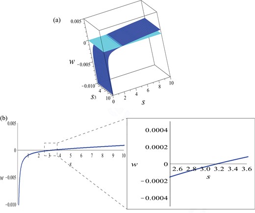
Since we are looking for the minimum positive speed with respect to s > 0 and s₃ > 0, in Fig. 12(a) we plot implicitly equation (5.8) in the |$\left (s, s_{3}, w\right )$|-space. Note that the steepness coefficient s₃ (for the ECM degradation profile) does not have any significant effect on the minimum positive wave speed w (of the invading u₁ and u₂ populations). For this reason, in Fig. 12(b) we plot the relation (5.8) in the |$\left (s, w\right )$|-plane for fixed s₃ > 0. We see that indeed we cannot have a travelling wave with positive speed unless the wave has a steepness s > 3.17. Moreover, faster waves have higher steepness.

Fig. 12.

Plot of the relation (5.8) for q_r = 0.0005, q_a = 0.00025 and the rest of the model parameters as given in Table 2. The plot shows the relation between the speed and the steepness of the travelling waves in the (a) |$\left (s, s_{3}, w\right )$|-space; (b) |$\left (s, w\right )$|-plane.

Finally, we are interested in investigating how the speed of the invading waves correlates with their steepness, as we vary different model parameters. In Fig. 13(a) we see that a decrease in the diffusion coefficient D by one order of magnitude leads to a reduction in the velocity w > 0. In Fig. 13(b) we see that an increase in the mutation rate M (from 0.001 to 0.05) leads to a slightly lower velocity w > 0 and a higher steepness. (Note that for s > 100, the invading speed obtained for M = 0.001 and M = 0.05 is the same—not shown here.)

Fig. 13.

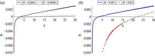
Plot of the relation (5.8) for q_r = 0.0005, q_a = 0.00025, and the rest of the model parameters as given in Table 2, as we vary: (a) diffusion coefficient D: D = 10⁻⁴ (black solid curve) and D = 10⁻⁵ (red dashed curve); (b) mutation rate M: M = 0.001 (blue solid curve) and M = 0.05 (red dashed curve).

6. Conclusions and discussion

In this paper we introduced a model of integro-differential equations describing the dynamics of two cancer cell populations: a ‘normal’ cell population that exhibits both random and directed movement, and a ‘mutant’ cell population that exhibits only directed movement. The model incorporated both nonlocal cell–cell interactions and cell–matrix interactions. Moreover, unlike other models in the literature, in our model these interactions were not constant but depended on the cellular level of integrins.

Linear stability analysis of the non-dimensional model showed that aggregations could arise only via real bifurcations (the system could not exhibit Hopf bifurcations). Numerical results showed that these aggregations were described by a large number of stationary pulses (e.g. 13 pulses corresponding to the critical unstable wave number k₁₃). Moreover, numerics also showed the existence of travelling waves. We investigated the speed of these waves, which seemed to be affected by the diffusion coefficient and the mutation rate of cells.

The rate at which cancer cells mutate seemed to play a critical role in our model. In Figs 6 and 7 (as well as Figs 8 and 10) we showed that depending on the magnitude of the mutation rate, either the u₁ or the u₂ cell populations can be eliminated (or, in some cases they can co-exist—see Figs 4 and 8). The existence of these dominant behaviours exhibited by the u₁ or u₂ populations are consistent with the principle of competitive exclusion of clonal sub-populations in heterogeneous tumours (Egan et al., 2012; Keats et al., 2012; Leith et al., 1989). In Fisher et al. (2013) the authors interpreted the experimental data, which showed suppression and reappearance of cancer clones in myeloma patients (Keats et al., 2012) and chronic lymphocytic leukaemia patients (Schuh et al., 2012), by suggesting that two subclones can exist in a dynamic equilibrium. While all these experimental studies record the survival/suppression of tumour clones in various cancers, they do not offer a mechanistic explanation for the factors that could lead to these behaviours. In contrast, our numerical results (see Figs 6 and 7, 8 and 10) offer such a mechanistic explanation by identifying the magnitude of the mutation rate as a factor that could explain the experimentally observed suppression and reappearance of cancer clones.

This issue of cancer heterogeneity has significant implications on cancer drug therapies, since it can lead to drug resistance. For example, clinical studies have shown the emergence of imatinib-resistant mutation clones in patients with chronic myeloid leukaemia, which can co-exist with subclones that carry different imatinib-resistant mutations in treatment-naïve patients (Shah et al., 2002). Overall, these clinical observations suggest that a single drug might not be successful in treating a genetically heterogeneous tumour, since sub-populations of cancer cells with drug-resistant mutations could become dominant, thus leading to therapeutic failure.

We note that the spatial distribution of the two cancer sub-populations, with the original u₁ population in the centre of the aggregation and the mutated u₂ clones towards the edges of the aggregation (see Fig. 5 for |$t\in \left [0, 10\right ]$| or Fig. 6 for |$t\in \left [100, 300\right ]$|⁠), is consistent with experimental studies on the spatial relationship between clonal sub-populations of hepatocellular carcinoma (HCC) tumour (Ling et al., 2015). In this experimental study, the authors investigated the clonal diversity of a HCC-15 tumour (and the spatial distribution of these clones), and showed the ancestral clones being positioned in the middle of the tumour, with the descendant clones radiating outward.

The numerical results of the model presented in this paper show that cell–cell/cell–matrix adhesion combined with cell proliferation (in the presence of cell competition) and cell mutation, can impact which tumour clones survive (see Figs 4–8 and 10). Therefore, our model puts forward the idea that in order to predict the emergence of a particular cancer clone, we should first quantify cell–cell and cell–matrix adhesive interactions for the various tumour clones, and their proliferative capacities.

In this paper we focused on a 1D model. However, real life cell dynamics occurs in 2D or 3D. In Appendix A we extended model (2.22) to two spatial dimensions. Moreover, to verify if the linear stability results for the 1D model (2.22) were valid also in 2D, we applied linear stability analysis. We showed that for similar kernels, we obtained similar dispersion relations with no imaginary parts (and hence no Hopf bifurcations). Therefore, we expect that the 2D model (A1) would exhibit stationary pulses similar to the ones exhibited by the 1D model (2.22). Future work will consider extending the numerical results in 2D.

Acknowledgements

V. B. acknowledges support from an Engineering and Physical Sciences Research Council (UK) grant number EP/L504932/1. R. E. acknowledges support from an Engineering and Physical Sciences Research Council (UK) grant number EP/K033689/1.

Appendix A. Extension of the model to two dimensions

The derivation of the model in two dimensions is a straightforward extension of the methods used in Section 2.2. Let |$\varOmega \subset \mathbb {R}^{2}$| denote again the bounded spatial domain and |$I_{T}=\left [0, +\infty \right )$| be the time interval. We only consider a rectangle with periodic boundary conditions. We denote again by |$\underline {u}\left (\underline {\mathbf {x}}, t\right )=\left (u_{1}\left (\underline {\mathbf {{x}}}, t\right ), u_{2}\left (\underline {\mathbf {{x}}}, t\right )\right )^{\top }$| the vector-valued cancer cell density of the two populations, by |$f\left (\underline {\mathbf {{x}}}, t\right )$| the ECM density and by |$c\left (\underline {\mathbf {{x}}}, t\right )$| the integrin density. Our 2D system, obtained after non-dimensionalization, is given by

\begin{align} \frac{\partial u_{1}}{\partial t}=D\Delta u_{1}-\nabla\cdot\left(u_{1}\underline{F_{1}}\left[{\kern.6pt}\underline{u}, f, c\right]\right)-Mu_{1}+r_{1}u_{1}\left(1-u_{1}-u_{2}\right), \end{align}

(A.1a)

\begin{align} \frac{\partial u_{2}}{\partial t}=-\nabla\cdot\left(u_{2}\underline{F_{2}}\left[{\kern.6pt}\underline{u}, f, c\right]\right)+Mu_{1}+r_{2}u_{2}\left(1-u_{1}-u_{2}\right), \end{align}

(A.1b)

\begin{align} \frac{\partial f}{\partial t}=-\alpha u_{1}{\kern2pt}f-\beta u_{2}{\kern2pt}f, \end{align}

(A.1c)

\begin{align} \frac{\partial c}{\partial t}=p_{1}u_{1}+p_{2}u_{2}-qc. \end{align}

(A.1d)

We now assume that cells interact with each other within a circle of sensing radius R > 0. Therefore, the nonlocal terms, |$\underline {F_{i}}\left [\kern2pt\underline {u}, f, c\right ], i=1, 2$|⁠, are given as in Gerisch & Chaplain (2008) by the following relations

\begin{align} \underline{F_{i}}\left[{\kern.6pt}\underline{u}, f, c\right]&:=\frac{1}{R}{\int_{0}^{R}}\int_{0}^{2\pi} \underline{\eta}\left(\theta\right) K_{i}\left(r\right)g_{i}\left(\underline{u}\left(\underline{\mathbf{{x}}}+r\underline{\eta}\left(\theta\right), t\right), f\left(\underline{\mathbf{{x}}}+r\underline{\eta}\left(\theta\right), t\right), c\left(\underline{\mathbf{{x}}}, t\right)\right)r\ \mathrm{d}\theta\ \mathrm{d}r, \end{align}

(A.2)

where |$\underline {\eta }\left (\theta \right ):=\left (\cos \theta , \sin \theta \right )^{\top }$| is the unit outer normal vector corresponding to angle θ. The functions g_i, i = 1, 2, are given by

\begin{align} g_{i}\left(\underline{u}\left(\underline{\mathbf{{x}}}, t\right)\!, f\left(\underline{\mathbf{{x}}}, t\right)\!, c\left(\underline{\mathbf{{x}}}, t\right)\right)=S_{i} \left(c\right)u_{i}\left(\underline{\mathbf{{x}}}, t\right)+S\left(c\right) u_{j}\left(\underline{\mathbf{{x}}}, t\right)+C_{i}\left(c\right)f\left(\underline{\mathbf{{x}}}, t\right)\!,\;i, j=1, 2,\;i\neq j. \end{align}

(A.3)

Linear stability analysis for the two dimensional model. Following the same approach as in the one-dimensional case (see Section 3), we analyse the stability of the steady states given by the relation (3.2). To this end, we let

\begin{align*} &u_{1}\left(\underline{\mathbf{{x}}},t\right)=u_{1}^{\ast}+A_{u_{1}}e^{i\underline{k}\;\underline{\mathbf{{x}}}+\lambda t},\; u_{2}\left(\underline{\mathbf{{x}}},t\right)=u_{2}^{\ast}+A_{u_{2}}e^{i\underline{k}\;\underline{\mathbf{{x}}}+\lambda t}, \; f\left(\underline{\mathbf{{x}}},t\right)=f^{\ast}+A_{f}e^{i\underline{k}\;\underline{\mathbf{{x}}}+\lambda t},\\ &c\left(\underline{\mathbf{{x}}},t\right)=c^{\ast}+A_{c}e^{i\underline{k}\;\underline{\mathbf{{x}}}+\lambda t}, \; \;\text{with}\; \;\lvert A_{u_{1}}\rvert, \lvert A_{u_{2}}\rvert, \lvert A_{f}\rvert, \lvert A_{c}\rvert\ll1. \end{align*}

Here, |$\underline {k}=\left (k_{1}, k_{2}\right )$| is a perturbation wave vector and λ is the linear growth rate. Substituting these expressions into model (A1) we obtain the following linearized system:

\begin{align*} \lambda A_{u_{1}}e^{i\underline{k}\;\underline{\mathbf{{x}}}+\lambda t}=&-\lvert\underline{k}\rvert^{2}D A_{u_{1}}e^{i\underline{k}\;\underline{\mathbf{{x}}}+\lambda t}-\frac{u_{1}^{\ast}}{R}i\underline{k}e^{i\underline{k}\;\underline{\mathbf{{x}}}+\lambda t}S_{1}\left(c^{\ast}\right)A_{u_{1}}{\int_{0}^{R}} \int_{0}^{2\pi} \underline{\eta}\left(\theta\right) K\left(r\right)e^{i\underline{k}\;r\underline{\eta}\left(\theta\right) }r\ \mathrm{d}\theta\ \mathrm{d}r\\ &-\frac{u_{1}^{\ast}}{R}i\underline{k}e^{i\underline{k}\;\underline{\mathbf{{x}}}+\lambda t}\left(S\left(c^{\ast}\right)A_{u_{2}}+C_{1}\left(c^{\ast}\right)A_{f}\right){\int_{0}^{R}} \int_{0}^{2\pi} \underline{\eta}\left(\theta\right) K\left(r\right)e^{i\underline{k}\;r\underline{\eta}\left(\theta\right) }r\ \mathrm{d}\theta\ \mathrm{d}r\\&-MA_{u_{1}}e^{i\underline{k}\;\underline{\mathbf{{x}}}+\lambda t}+r_{1}A_{u_{1}}e^{i\underline{k}\;\underline{\mathbf{{x}}}+\lambda t}\left(1-2u_{1}^{\ast}-u_{2}^{\ast}\right)-r_{1}u_{1}^{\ast}A_{u_{2}}e^{i\underline{k}\;\underline{\mathbf{{x}}}+\lambda t},\\ \lambda A_{u_{2}}e^{i\underline{k}\;\underline{\mathbf{{x}}}+\lambda t}=&-\frac{u_{2}^{\ast}}{R}i\underline{k}e^{i\underline{k}\;\underline{\mathbf{{x}}}+\lambda t}\left( S_{2}\left(c^{\ast}\right)A_{u_{2}}\!+S\left(c^{\ast}\right)A_{u_{1}}\!+C_{2}\left(c^{\ast}\right)A_{f}\right){\int_{0}^{R}} \int_{0}^{2\pi} \!\underline{\eta}\left(\theta\right) K\left(r\right)e^{i\underline{k}\;r\underline{\eta}\left(\theta\right) }r\ \mathrm{d}\theta\ \mathrm{d}r\\ &+r_{2}A_{u_{2}}e^{i\underline{k}\;\underline{\mathbf{{x}}}+\lambda t}\left(1-u_{1}^{\ast}-2u_{2}^{\ast}\right)-r_{2}u_{2}^{\ast}A_{u_{1}}e^{i\underline{k}\;\underline{\mathbf{{x}}}+\lambda t},\\ \lambda A_{f}e^{i\underline{k}\;\underline{\mathbf{{x}}}+\lambda t}=&-\alpha\left(A_{u_{1}}e^{i\underline{k}\;\underline{\mathbf{{x}}}+\lambda t}{\kern2pt}f^{\ast}+u_{1}^{\ast}A_{f}e^{i\underline{k}\;\underline{\mathbf{{x}}}+\lambda t}\right)-\beta \left(A_{u_{2}}e^{i\underline{k}\;\underline{\mathbf{{x}}}+\lambda t}{\kern2pt}f^{\ast}+u_{2}^{\ast}A_{f}e^{i\underline{k}\;\underline{\mathbf{{x}}}+\lambda t}\right),\\ \lambda A_{c}e^{i\underline{k}\;\underline{\mathbf{{x}}}+\lambda t}=&\ p_{1} A_{u_{1}}e^{i\underline{k}\;\underline{\mathbf{{x}}}+\lambda t}+p_{2} A_{u_{2}}e^{i\underline{k}\;\underline{\mathbf{{x}}}+\lambda t}-q A_{c}e^{i\underline{k}\;\underline{\mathbf{{x}}}+\lambda t}. \end{align*}

Therefore, we finally have

\begin{align*} \lambda A_{u_{1}}=&-\lvert\underline{k}\rvert^{2}D A_{u_{1}}-\frac{i\underline{k}u_{1}^{\ast}}{R}\left[S_{1}\left(c^{\ast}\right) A_{u_{1}}\!+S\left(c^{\ast}\right)A_{u_{2}}\!+\!C_{1}\left(c^{\ast}\right)A_{f}\right]\underline{\hat{K}}\left(\underline{k}\right)-M A_{u_{1}}\!+r_{1}A_{u_{1}}\left(1\!-2u_{1}^{\ast}-u_{2}^{\ast}\right)\nonumber\\&-r_{1}u_{1}^{\ast}A_{u_{2}},\\ \lambda A_{u_{2}}=&-\frac{i\underline{k}u_{2}^{\ast}}{R}\left[S_{2}\left(c^{\ast}\right)A_{u_{2}}\!+S\left(c^{\ast}\right)A_{u_{1}}\!+C_{2}\left(c^{\ast}\right)A_{f}\right]\underline{\hat{K}}\left(\underline{k}\right)+M A_{u_{1}}\!+r_{2}A_{u_{2}}\left(1\!-u_{1}^{\ast}\!-2u_{2}^{\ast}\right)-r_{2}u_{2}^{\ast}A_{u_{1}},\\ \lambda A_{f}=&-\alpha\left(A_{u_{1}}{\kern2pt}f^{\ast}+u_{1}^{\ast}A_{f}\right)-\beta \left(A_{u_{2}}{\kern2pt}f^{\ast}+u_{2}^{\ast}A_{f}\right),\\ \lambda A_{c}=&\ p_{1}A_{u_{1}}+p_{2} A_{u_{2}}-q A_{c}, \end{align*}

where |$\underline {\hat {K}}\left (\underline {k}\right )={\int _{0}^{R}} \int _{0}^{2\pi } \underline {\eta }\left (\theta \right ) K\left (r\right )e^{i\underline {k}\;r\underline {\eta }\left (\theta \right ) }r\ \mathrm {d}\theta\, \mathrm {d}r$| is the Fourier transform of the kernel |$K\left (\underline {\mathbf {{x}}}\right )$|⁠. Note that |$\underline {\hat {K}}\left (\underline {k}\right )$| corresponds to the 1D Fourier sine transform (see Section 3), since |$\hat {K}^{s}\left (k\right )={\int _{0}^{R}}K\left (r\right )\sin \left (kr\right )\ \ \mathrm {d}r=\frac {1}{2i}{\int _{0}^{R}}K\left (r\right )\left (e^{ikr}-e^{-ikr}\right )\ \mathrm {d}r$|⁠.

As in 1D case, for the steady state |$\left (0, 0, f^{\ast }, 0\right ),\ f^{\ast }\geq 0$|⁠, we obtain the eigenvalues

\begin{align} \lambda_{1}=0,\enspace \lambda_{2}=-\lvert\underline{k}\rvert^{2}D-M+r_{1},\enspace \lambda_{3}=r_{2}>0 \ \ \text{and}\ \ \lambda_{4}=-q<0. \end{align}

(A.4)

For the steady state |$\left (0, 1, 0, p_{2}/q\right )$| we obtain the eigenvalues

\begin{align} \lambda_{1}=-\beta <0,\enspace \lambda_{2}=-\lvert\underline{k}\rvert^{2}D-M<0,\enspace \lambda_{3}=-S_{2}\left(c^{\ast}\right)Y\left(\underline{k}\right)-r_{2}\ \ \text{and}\ \ \lambda_{4}=-q<0, \end{align}

(A.5)

where |$Y\left (\underline {k}\right )=\frac {i\underline {k}}{R}\underline {\hat {K}}\left (\underline {k}\right )$|⁠, with |$K\left (\underline {\mathbf {{x}}}\right ):=q_{a}K_{a}\left (\underline {\mathbf {{x}}}\right )-q_{r}K_{r}\left (\underline {\mathbf {{x}}}\right )$|⁠. Here K_a and K_r are the attraction and repulsion kernels, and q_a and q_r are the constants representing the magnitudes of the attraction and repulsion interactions, respectively. For simplicity we choose the following 2D interaction kernel

\begin{align} K\left(\underline{\mathbf{{x}}}\right)=\frac{q_{a}\vert\underline{\mathbf{{x}}}\rvert}{2\pi {m^{2}_{a}}}\exp\left(-\vert\underline{\mathbf{{x}}}\rvert^{2}\left/\left(2{m^{2}_{a}}\right)\right.\right)-\frac{q_{r}\vert\underline{\mathbf{{x}}}\rvert}{2\pi {m^{2}_{r}}}\exp\left(-\vert\underline{\mathbf{{x}}}\rvert^{2}\left/ \left(2{m^{2}_{r}}\right)\right.\right), \end{align}

(A.6)

which corresponds to the 1D kernel (3.15). The Fourier transform of the above kernel is given by the following relation

\begin{align} \underline{\hat{K}}\left(\underline{k}\right)=\left(q_{a}i{m_{a}^{2}}k_{1}e^{-\frac{{m_{a}^{2}}\lvert\underline{k}\rvert^{2}}{2}}-q_{r}i{m_{r}^{2}}k_{1}e^{-\frac{{m_{r}^{2}}\lvert\underline{k}\rvert^{2}}{2}}, q_{a}i{m_{a}^{2}}k_{2}e^{-\frac{{m_{a}^{2}}\lvert\underline{k}\rvert^{2}}{2}}-q_{r}i{m_{r}^{2}}k_{2}e^{-\frac{{m_{r}^{2}}\lvert\underline{k}\rvert^{2}}{2}}\right). \end{align}

(A.7)

Therefore, the steady state |$\left (0, 1, 0, p_{2}/q\right )$| is unstable provided that the real part of the eigenvalue λ₃ satisfies

\begin{align} Re\left(\lambda_{3}\left(\underline{k}\right)\right)=&-r_{2}+\frac{\lvert\underline{k}\rvert^{2}s_{2}^{\ast}}{R}\left(1+\tanh\left(a_{2}\frac{p_{2}}{q}\right)\right)\left(q_{a}{m_{a}^{2}}e^{-\frac{{m_{a}^{2}}\lvert\underline{\underline{k}}\rvert^{2}}{2}}-q_{r}{m_{r}^{2}}e^{-\frac{{m_{r}^{2}}\lvert\underline{k}\rvert^{2}}{2}}\right)>0. \end{align}

(A.8)

This expression is similar to the one obtained in the 1D case (see equation (3.17)). Therefore we deduce that there is a range of |$\underline {k}\text{-}$|values for which |$Re\left (\lambda _{3}\left (\underline {k}\right )\right )$| is positive, and thus spatial aggregations could develop also for the 2D model (A1) when applying small spatial perturbations of the steady state |$\left (0, 1, 0, p_{2}/q\right )$|⁠.

Appendix B. A structured-population model for cancer–ECM interactions via integrins

As mentioned at the end of Section 2.1, we can modify model (2.13)–(2.16) to describe in a more natural way the connection between the macroscale movement of cells and the microscale dynamics of integrins bound to cell surfaces. To this end, we assume that the two cancer cell populations depend not only on time (t) and space (x), but also on an internal variable that characterizes the level of bound integrins: u_i(x, t, c). The new mesoscale model for the dynamics of cancer cell populations structured by cell-bound integrins is given by the following equations:

\begin{align} \frac{\partial u_{1}}{\partial t}=D\frac{\partial^{2} u_{1}}{\partial x^{2}}-\frac{\partial}{\partial x} \left(u_{1}F_{1}[{\kern.6pt}\underline{u}, f, c]\right)-\frac{\partial}{\partial c}\left(u_{1}(p_{1}u_{1}+p_{2}u_{2}-qc)\right) -Mu_{1}+r_{1}u_{1}\left(1-u_{1}-u_{2}\right), \end{align}

(B.1a)

\begin{align} \frac{\partial u_{2}}{\partial t}=-\frac{\partial}{\partial x} \left(u_{2}F_{2}[{\kern.6pt}\underline{u}, f, c]\right) -\frac{\partial}{\partial c}\left(u_{2}(p_{1}u_{1}+p_{2}u_{2}-qc)\right)+Mu_{1}+r_{2}u_{2}\left(1-u_{1}-u_{2}\right), \end{align}

(B.1b)

\begin{align} \frac{\partial f}{\partial t}=-\alpha u_{1}{\kern2pt}f-\beta u_{2}{\kern2pt}f. \end{align}

(B.1c)

The nonlocal terms |$F_{1}[\kern2pt\underline {u},f,c]$| and |$F_{2}[\kern2pt\underline {u},f,c]$| are described by equations (2.10) and (2.11), respectively. The microscale evolution of the internal state variable c is described by differential equation (2.16):

\begin{align} \frac{\partial c}{\partial t}=p_{1}u_{1}+p_{2}u_{2}-qc. \end{align}

(B.2)

The incorporation of this internal cell structure c into the mesoscopic model (B1) follows the same approach as in Erban & Othmer (2004, 2005); Xue et al. (2011); Lorenz & Surulescu (2014); Engwer et al. (2015); Perthame et al. (2016); Engwer et al. (2017); Hunt & Surulescu (2017).

One can eliminate the derivative ∂/∂c from equations (B1a)–(B1b) by integrating these equations over c, and obtaining new macroscopic equations defined in terms of the averaged tumour cell variables |$U_{1,2}(x,t)=\int u_{1,2}(x,t,c)\ \text {d}c$| (Erban & Othmer, 2005; Engwer et al., 2015; Domschke et al., 2107). Other studies obtained different macroscopic limits of the mesoscopic structured-population models by considering the assumption that the internal (structure) variable evolves on a much faster time scale that is described by a small parameter (Perthame et al., 2016). If we would take the same approach and assume that the integrin dynamics is much faster compared to the dynamics of cancer cells and ECM (note that in Table 2 the production rates of integrins by u₁ and u₂ cells are estimated, due to a lack of available data), then the time-evolution of integrins would be given by

\begin{align} \varepsilon \frac{\partial c}{\partial t}=p_{1}u_{1}+p_{2}u_{2}-qc, \end{align}

(B.3)

which, to leading order, gives rise to the following steady-state equation: c = (1/q)(p₁u₁(x) + p₂u₂(x)). If we substitute this state into (B1) we recover model (2.22), with the exception of equation (2.22d) which is now a steady-state equation.

We note here that while different ‘microscale–macroscale’ models (Stinner et al., 2014, 2015, 2016; Meral et al., 2015a,b) and ‘mesoscale’ models (Lorenz & Surulescu, 2014; Engwer et al., 2015; Perthame et al., 2016; Engwer et al., 2017; Hunt & Surulescu, 2017) for tumour-ECM interactions via integrins have been developed over the last two decades, to our knowledge there are not many studies that compare and contrast the outcomes of different ways the integrins are incorporated into these different models.

A comparison between the effects of integrins on the dynamics of the structured-population model (B1) and the original model (2.22) (both assuming heterogeneous cell populations), including an investigation into the possibility of having travelling wave solutions for the structured model (B1), will be the subject of a future study. (Such an investigation is beyond the scope of this study due to its complexity, which would increase considerably the length of this paper.)