Mathematical modelling of glob-driven tear film breakup

Abstract

Evaporation is a recognized contributor to tear film thinning and tear breakup (TBU). Recently, a different type of TBU is observed, where TBU happens under or around a thick area of lipid within a second after a blink. The thick lipid corresponds to a glob. Evaporation alone is too slow to offer a complete explanation of this breakup. It has been argued that the major reason of this rapid tear film thinning is divergent flow driven by a lower surface tension of the glob (via the Marangoni effect). We examine the glob-driven TBU hypothesis in a 1D streak model and axisymmetric spot model. In the model, the streak or spot glob has a localized high surfactant concentration, which is assumed to lower the tear/air surface tension and also to have a fixed size. Both streak and spot models show that the Marangoni effect can lead to strong tangential flow away from the glob and may cause TBU. The models predict that smaller globs or thinner films will decrease TBU time (TBUT). TBU is located underneath small globs, but may occur outside larger globs. In addition to tangential flow, evaporation can also contribute to TBU. This study provides insights about mechanism of rapid thinning and TBU which occurs very rapidly after a blink and how the properties of the globs affect the TBUT.

tear film, thin film, Marangoni effect, dry eye, tear breakup

1. Introduction

Dry eye syndrome (DES) is one of the most common reasons for seeking eye care (Stapleton et al., 2015). It can significantly affect clear vision, cause discomfort and thus diminish quality of life (Mertzanis et al., 2005; Miljanović et al., 2007). For example, it is estimated that at least 3.2 million woman aged over 50 in the USA are affected by DES in 2003 (Schaumberg et al., 2003) and the number is expected to increase as baby boomers age (Akpek & Smith, 2013). Thus, further understanding of DES is needed to improve treatments for this common condition.

One of the core mechanisms of DES is tear film instability or tear breakup (TBU), which causes the tears to disrupt quickly and thus poorly coat the surface of the eye (Anonymous, 2007). The tear film is typically considered a three-layered film. It is composed of a very thin lipid layer on its surface over a relatively thick aqueous layer with a bound mucin layer (often called a glycocalyx) on the bottom. The lipid layer has an outer layer of non-polar lipid and an inner layer of polar lipid at the interface with the aqueous layer. The non-polar lipid layer is generally believed to be a barrier to evaporation (Mishima & Maurice, 1961; Paananen et al., 2014), whilst the polar lipid layer acts as a surfactant which can drive flow in the aqueous layer (Johnson & Murphy, 2004; McCulley & Shine, 1997). Examination of the lipid layer through the use of a high resolution microscopy suggests that differences in lipid layer structure may correlate with DES (Craig & Tomlinson, 1997; King-Smith et al., 2011); x-ray scattering methods have revealed some details about structure as well (Leiske et al., 2012; Rosenfeld et al., 2013).

The aqueous layer is largely water (Holly, 1973) and is normally treated as a Newtonian fluid i.e. close to water in its properties (Braun, 2012). However, the aqueous layer contains ions from salts and a number of large proteins and mucins (Bron et al., 2004); the large molecules help make whole tears slightly shear thinning (Nagyová & Tiffany, 1999). The glycocalyx is a hydrophilic forest of glycosylated proteins that attract water and helps moisturize the corneal surface by making it wettable (Gipson, 2004). A damaged glycocalyx has been hypothesized to promote TBU and tear film instability (Sharma & Ruckenstein, 1985; Gipson, 2004; Yokoi & Georgiev, 2013b; Yanez-Soto et al., 2014).

The Dry Eye Workshop (DEWS; Anonymous, 2007) has divided DES into two classes: aqueous tear-deficient dry eye (ADDE) and evaporative dry eye (EDE). The core mechanisms of DES have been widely accepted to be tear hyperosmolarity and tear film instability. Tear hyperosmolarity can be the result of either water evaporation or deficiency of tear generation (Lemp, 2007). High osmolarity in the tear film can generate stress to ocular surface and can cause inflammation and ocular surface damage (Li et al., 2006). Tear osmolarity has been proposed as the standard (Farris, 1994; Lemp et al., 2011) for a DES test due to the fact that a dry eye has a higher osmolarity (Tomlinson et al., 2006). For the purposes of this article, we define tear film instability or TBU to be the state when the tear film becomes sufficiently thin that the tear/air interface reaches the top of the glycocalyx at the ocular surface (King-Smith et al., 2017). The severity of tear film instability is thought to be indicated by a short TBU time (TBUT), meaning that the tear film becomes unstable rapidly (Cho et al., 1992). Since excessive evaporation can play an important role in both types of DES, the two core mechanisms may not be independent.

Osmolarity is defined as the combined concentration of osmotically active solutes, primarily salts and protein in the aqueous layer (Stahl et al., 2012; Braun, 2012). When an osmotic difference exists between the tear film and corneal epithelium, osmotic flow is generated which is typically from the cornea to the tear film (Peng et al., 2014; Braun et al., 2015). Osmolarity is typically difficult to measure in the tear film. Older methods require either a complicated procedure or a large sample size of tears (Gilbard et al., 1978; Farris, 1994). Recently, lab-on-a-chip technology has enabled a non-invasive and quick test that measures osmolarity in the inferior meniscus. By using a 50-nL tear sample, it can provide a result within seconds and this new technology has enabled a proposed cut-off value for the diagnosis of DES (Lemp et al., 2011). There is further work to be done to correlate tear film osmolarity with signs and symptoms of DES (Sebbag et al., 2016).

King-Smith et al. (2008) proposed that there are three fluxes of water that may be significant on the anterior surface of the eye: evaporative, osmosis and tangential. Water may be lost to the air and environment outside the eye via evaporation of water from the tear film. As discussed above, water may be supplied to the tear film via an osmotic flux by osmolarity differences across the tear/corneal interface. Tangential flow is along the corneal surface and it can be driven by: (i) capillarity, which are pressure differences due to surface tension and curvature of the tear/air interface (Oron et al., 1997); (ii) the Marangoni effect, where surface concentration differences generate shear stresses on the tear/air interface (Craster & Matar, 2009); and (iii) intermolecular forces like van der Waals forces (Winter et al., 2010; Zhang et al., 2004). Based on the direction of the tangential flow, it can be classified as either convergent or divergent. Convergent flow will push the tears into the center of the TBU region. Divergent flow will send tears outward from the center and thin the tear film.

All of the contributions to the flow that were discussed in the previous paragraph can affect tear film dynamics; the effects may be on different time and space scales however (Braun, 2012). Identifying each of the different effects in vivo is a major challenge; it is also a challenge to build and solve mathematical models that incorporate these effects, but advances have been made. We now turn to discussing these kinds of studies.

There are many different imaging methods to help study the dynamics of tears and TBU. King-Smith et al. (2017) recently reviewed five different imaging systems: (i) fluorescence for tear volume, (ii) reflection for tear film surface, (iii) interferometry for the thickness and structure of tear film lipid layer (TFLL), (iv) refraction for the shape of tear film surface and (v) thermal radiation for temperature distribution. Fluorescence is the most widely used method despite some quantitative uncertainty about absolute thickness measurement; however, when combined with other image methods, it can help study TBU dynamics and and mechanisms for its causes. For example, when combined with interferometry, aqueous layer dynamics can be correlated with TFLL dynamics to understand how they are intimately linked (King-Smith et al., 2013b). These studies have found that TBU occurs under both a thin and a thick lipid layer. Excessive evaporation can lead to TBU for very thin areas or holes in the TFLL, whilst the Marangoni effect has been proposed to explain TBU under globs of thick TFLL (King-Smith et al., 2013b). Simultaneous fluorescence and retroillumination images reveal the relation between tear film thickness and the surface structure of the tear film. Such combinations of simultaneous imaging, particularly including the TFLL, can help us determine the mechanisms of TBU more precisely (Braun et al., 2015). Additionally, the combination of fluorescence and thermal images can be used to study the effect of evaporation. Evaporation is thought to be a significant mechanism that cools the tear film during the interblink. Strong correlation between fluorescent and thermal imaging has been observed, which supports the conclusion that evaporation is a non-negligible cause of TBU (Kamao et al., 2011; Su et al., 2014).

A variety of mathematical models of the tear film have been reviewed in Braun (2012). Most models of tear film are 1D single-layer models, with the common simplifications that consider the aqueous layer to be a Newtonian fluid (Wong et al., 1996; Sharma, 1998a; Miller et al., 2002; Braun & Fitt, 2003), treat the TFLL as an insoluble surfactant monolayer (Berger & Corrsin, 1974; Jones et al., 2006; Aydemir et al., 2010) and assume the substrate (corneal surface) under the tear film to be flat impermeable surface (Braun et al., 2012). These simplified models have been able to investigate important effects tear dynamics over the open surface of the eye, such as evaporation into the air (Winter et al., 2010), heat transfer within the tear film and outside environment (Scott, 1988), Van der Waals forces acting on the aqueous layer (Oron & Bankoff, 1999; Israelachvili, 2011; Zhang et al., 2004), osmosis across the corneal surface (Braun, 2012), Marangoni effects induced by varying concentration of polar lipid (Aydemir et al., 2010; Berger & Corrsin, 1974), complete blink cycles (Braun & King-Smith, 2007) and partial blink cycles (Heryudono et al., 2007). Related 2D models of tear film dynamics have also been developed by Maki et al. (2010a), Maki et al. (2010b) and Li et al. (2014, 2016).

In many mathematical models, the lipid layer is usually simplified to be a polar lipid monolayer, where the concentration gradient can induce a Marangoni flow but it can also affect evaporation. Some models have focused on evaporation based on the amount of lipid present in the TFLL. Siddique & Braun (2015) built a 1D evaporative model, where evaporation depends on pressure, temperature and surfactant concentration. The model successfully captures TBU induced by evaporation, but cannot detect the increased evaporation rate caused by surfactant concentration. Peng et al. (2014) developed another 1D single-layer model, which captures TBU induced by the excessive evaporation due to a spatial variation in the thickness of a stationary lipid layer. The rupture of a hypothesized mobile precorneal mucus coating of 20–50 nm over the ocular epithelial surface was investigated by Zhang et al. (2004); their results indicated that, for a thin mobile mucus layer, van der Waals forces act significantly to disrupt the mucus layer and the corresponding TBUT matches the clinical TBUT for a dry eye and a healthy eye. Recently, Stapf et al. (2017) studied a model with two mobile Newtonian fluid layers, one an aqueous layer and the other the lipid layer, i.e. adapted from the prior model of Bruna & Breward (2014). This model has shown that the Marangoni effect due to lipid defects can reduce the lipid layer thickness, which subsequently allows elevated evaporation and then TBU.

There are other models that have studied the effect of polar lipids during and after a blink to investigate the distribution of lipids and the upward flow tears post blink. The earliest of these, to our knowledge, is the post-blink model (no-lid movement) of Berger & Corrsin (1974). Jones et al. (2006) studied models for the opening phase together the interblink starting from fully and half closed lid positions. Computed solutions for the interblink only indicate that a high concentration of lipid localized near the lower lid can spread upward rapidly and drag fluid in the aqueous layer upward. The high concentration of lipid near the lower lid is a result of lipid being pushed there by the descending upper lid during a blink. When the opening phase starting from a half blink is included with the interblink, the high concentration of lipid occurs at the center of eye, and as a result, the concentration gradient of lipid causes rapid thinning in the area between the middle of the open domain and upper lid. Aydemir et al. (2010) studied a mathematical model that simulates eye blink with a moving upper lid and concluded that the Marangoni flow caused by the variation of lipid concentration can drive tears from the lower meniscus to the upper cornea, which thickens the entire tear film. By reducing the initial concentration of the polar lipid, the tear film becomes thinner. The simulations match some experimental results from dry eyes and thus imply that people with dry eye symptoms have difficulty generating sufficient quantity and quality of lipid. Bruna & Breward (2014) included both polar and non-polar lipids in their model; they identified several promising limiting cases as well. The dynamics of their solutions was more complex than those of Aydemir et al. (2010), but similar conclusions were reached.

However, none of these models are specially designed to explain the rapid thinning where TBU happens at one or more locations right after the eye opens. The simultaneous imaging of fluorescein and lipid layer thickness shows that dark spots (TBU regions) appear within 4 s and appear to be underneath relative thick areas of lipid, which we call globs (King-Smith et al., 2013b). Different mechanisms for this type of TBU have been proposed: one is divergent tangential flow due to differences in surfactant concentration differences (King-Smith et al., 2008) and another is decreased wettability of the cornea (Sharma & Ruckenstein, 1985, 1986; Sharma, 1998b; Yokoi & Georgiev, 2013a,b; Yanez-Soto et al., 2015). The divergent tangential flow mechanism is driven by the Marangoni effect, where surface concentration differences generate shear stresses that cause flow away from areas of high concentration. This hypothesis seems to be the only possible contribution to rapid TBU amongst the three component flows of tear thinning listed above. Firstly, osmotic flow is too small to slow this rapid thinning (Nichols et al., 2005). Secondly, evaporation is too slow to account for rapid TBU, except possibly in the case of severe ADDE with a very thin tear film. It takes at least 8 s to observe a dark spot for a 3.5 μm aqueous layer with an evaporation rate of 25 μm/min. However, TBUT can be as short as 0.2 s, but the highest observed evaporation rate is 25 μm/min (King-Smith et al., 2010). Recently, Yokoi & Georgiev (2013a) and Yokoi & Georgiev (2013b) have proposed that dewetting of the ocular surface can explain roughly-circular rapid breakup; they propose that an area of highly hydrophobic surface may exist due to a faulty glycocalyx which leads to rapid TBU. Under this assumption, the non-wetted ocular surface should correspond to a fixed location on the epithelial surface for the dark spot after the next blink. However, Fig. 1 shows that, for our data, dark spots were observed at different positions in the fluorescence images after each blink; this implies that Marangoni-driven tangential flow may provide an explanation for many TBU events with rapid thinning.

Fig. 1.

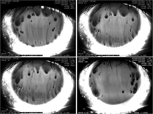
Time sequence of spot breakup (from the left to the right, from the top to the bottom). A dark spot forms 0.14 s after the first blink. The dark region then spreads downwards with unmoved dark center in the following two images 1.01 s and 2.01 s after first blink, resp. The lower right image shows that after the second blink, dark spots form again after 0.14 s in different locations.

In this article, we use two mathematical models to test the hypothesis that globs can cause a tangential flow, which subsequently drives TBU near the glob. One model is for 1D streaks, using the terminology of Bitton & Lovasik (1998), and the other is axisymmetric, for circular spots. In both models, we simulate the globs’ different composition by assuming that the glob has a higher surfactant concentration than the surrounding tear/air interface. Increased surfactant concentration is assumed to lower the tear film surface tension; this is how the model incorporates the Marangoni effect. By choosing the appropriate length and timescales, tear film thickness, other quantities, we simplify the full set of governing equations and boundary conditions to two simple, non-linear partial differential equations (PDEs) using lubrication theory (Oron et al., 1997; Craster & Matar, 2009). Both models are solved in the local region for the tear film thickness (h), the pressure (p) inside the film and insoluble surfactant concentration (⁠|$\varGamma$|⁠). Using reasonable choices for the parameters, TBUT is matched with clinical experiments. The effect of parameters on TBU like domain size, surface tension gradient, evaporation flux, glob size and tear film thickness are also examined. A comparison between the 1D streak model and spot model is also included. In both models, the results show that our assumptions for the glob lead to strong tangential flow away from the glob and may cause TBU.

In Section 2, we provide sample results from clinical experiments and discuss our assumptions of our model. In Section 3, we derive the mathematical models. Corresponding numerical results of both models are shown in Section 4. Discussion and conclusions follow; some details are given in the appendices.

2. Glob-driven tear film breakup mechanism

King-Smith et al. have developed an optical system which can generate simultaneous images of fluorescence of the aqueous layer and TFLL interferometry in order to investigate the relationship between TBU and the dynamics of the TFLL. An outline of the method is given here; details can found in King-Smith et al. (2013b). A 5-μL drop of 2% fluorescein solution is instilled into the tear film. The tear film is then illuminated with light that has passed through a blue interference filter; the returning reflected light (blue) and fluorescent light (green) are split, filtered and then recombined to create side-by-side fluorescent and TFLL images. In these images, the darker regions indicate a thinner layer and brighter indicates thicker. In general, evaporation of the aqueous layer is more rapid for a thinner TFLL (King-Smith et al., 2010); this can lead to evaporative TBU on the order of tens of seconds as in Fig. 6 of King-Smith et al. (2013b). In that case, a localized, very thin lipid layer leads to TBU at that location in tens of seconds. This is a prototypical case that illustrates the cases analysed in evaporative TBU (Peng et al., 2014; Braun et al., 2015, 2017). However, in other cases, a thinner tear film is found under a corresponding thicker lipid layer and this kind of breakup occurred very rapidly after blink. Different mechanisms are proposed here to explain this latter type of TBU. The top row of Fig. 4 of King-Smith et al. (2013b) illustrates this case, where quite thin regions appear by 0.12 s post blink.

Fig. 1 shows a time sequence of fluorescein images of the rapid TBU. This case does not use simultaneous TFLL interferometry but only shows fluorescence; however, this is an excellent case to illustrate rapid TBU (King-Smith et al., 2013a). The upper left image indicates that TBU forms in 0.14 s after a blink; the dark spots indicate a thinner aqueous layer. Then, these dark spots seem to spread downwards within the next 2 s with the center unmoved. It seems that the thick lipid (glob) thins the tear film very rapidly following the blink and the thinned aqueous layer in the TBU region traps the lipid glob. The lower right image corresponds to the tear film 0.14 s after the second blink of the same subject. The tear film thins rapidly but TBU occurs in different locations on the cornea, which provides some evidence that the TBU may be driven by the Marangoni effect rather than dewetting of a defective corneal surface patch. Similar images have been shown by Yokoi & Georgiev (2013b) that may be due to van der Waals dewetting forces on an unwettable patch; however, the images that we observed seem more likely to be driven by the Marangoni effect. In this article, we examine the hypothesis that the tangential flow, driven by Marangoni effect due to the different composition or amount of lipid in a glob, is responsible for the rapid thinning (King-Smith et al., 2013b).

3. Model formulation

As in many models, e.g. (Braun, 2012), we consider the tear film which comprises a single layer of Newtonian fluid. The lipid layer is treated as an insoluble surfactant assumed to be polar lipids at the tear/air interface; all Marangoni effects are assumed to arise from this insoluble surfactant. The substrate under the tear film (corneal surface) is assumed to be flat based on the fact that tear film thickness (3–5 μm) is small compared to the average radius of curvature of the cornea (Carney et al., 1997; Braun, 2012, which has an average radius of about 7.8 mm). The glycocalyx is simplified to a cut-off thickness below which the tear film cannot thin, and water is transported freely across it. We define TBU in the model as when the thickness has become 0.25 μm, which is a representative thickness of the glycocalyx. The corneal surface is assumed to be impermeable; osmosis is too slow to affect the thinning of the tear film for the rapid TBU we seek to model here (Braun, 2012). A sketch of the situation is shown in Fig. 2. Because we are focused on simulating the Marangoni effect driven by globs, some further assumptions are made. Firstly, we incorporate the thick glob as a local spot or streak of polar lipid with higher concentration than the surrounding surface. Secondly, the glob is assumed to be of fixed spatial size but is deformable in the direction normal to the substrate. Thirdly, since TBU happens rapidly (less than a second), we neglect the change of the concentration of the polar lipid and assume that the glob has a fixed concentration. Then, the glob acts as a source of surfactant that supplies surfactant (polar lipid) that spreads out from the glob on the tear/air interface.

Fig. 2.

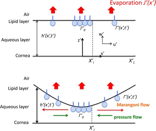
Schematic of the mechanism of glob-driven breakup with evaporation (J′), surfactant concentration (⁠|$\varGamma$|′) and tear film thickness (h′). |$X^{\prime }_{I}$| is the size of glob (thicker lipid) and |$X^{\prime }_{L}$| is the domain size to study this isolated glob model.

We include three aspects of tear film thinning in our model: (1) evaporation into the air; (2) divergent tangential flow driven by the transport of surfactant (Marangoni effect); (3) convergent tangential flow generated by the curvature of the tear film surface (pressure gradient flow from capillarity). We design our model to simulate a strong Marangoni flow which may lead to TBU in less than a second under reasonable conditions. Fig. 2 is a schematic of the 1D streak glob-driven model, which includes evaporation (J′), surfactant concentration (⁠|$\varGamma$|′), glob size |$\left(X^{\prime }_{I}\right)$| and domain size |$\left(X^{\prime }_{L}\right)$|⁠. As illustrated, the surfactant spreads outward from the edge of the glob/tear interface at |$X^{\prime }_{I}$| over the tear/air interface. The gradient of surfactant concentration generates a shear stress causing a tangential viscous flow, and that flow results in the formation of a depression near the center of the tear film. However, the distorted tear film surface will then generate a pressure gradient which will try to push back the aqueous; this capillarity-driven contribution flow is sometimes called a healing flow (King-Smith et al., 2013b). If the outward contribution to flow from the Marangoni effect is dominant over the capillary contribution to flow, then TBU will happen very rapidly, in well under a second. However, we also observed in both numerical and experimental results, the case where the tear film initially thins but then thickens again. In this case, the Marangoni contribution to flow is dominant at first, then as the concentration gradient decreases, the capillarity-driven healing flow becomes stronger and the aqueous layer under the glob eventually thickens. The relative size of the two contributions to flow depends on parameters like tear film thickness, glob size, surfactant concentration gradient and evaporation. The instability of the tear film is thus highly correlated to these properties of the tear film.

The Marangoni flow in this work causes a flow from a region of lower surface tension to a region of higher surface tension. To incorporate the Marangoni effect driven by the glob (thicker lipid), we assume that the glob has a lower surface tension due to its increased surfactant (polar lipid) concentration; hence, the shear stress generated at the tear/air interface (Craster & Matar, 2009) drags a tangential flow out of the glob. We assume that that the variation in surfactant concentration is not too large so that the equation of state for the surface tension depends linearly on surfactant concentration:

\begin{align} \sigma^{\prime}(\varGamma^{\prime}) = \sigma^{\prime}_{0} - |\sigma_{\varGamma}|_{0}\left(\varGamma^{\prime} - \varGamma^{\prime}_{0}\right)\!, \end{align}

(3.1)

where |$\sigma ^{\prime }_{0}$| is local surface tension and |$\varGamma$|′ is surfactant concentration. |$ |\sigma _{\varGamma }|_{0} = | \partial _{\varGamma }^{\prime } \sigma ^{\prime } |_{\varGamma ^{\prime }_{0}}$| is a positive constant which indicates the strength of the surfactant, we call it composition dependence here. In this way, we implemented the glob as a flexible patch of the tear/air interface with lower surface tension by assuming it has higher fixed surfactant concentration and a fixed size.

We outline the derivation of the 1D streak glob model in this section. The linear streak TBU is represented in Cartesian coordinates, and the axisymmetric spot TBU is represented cylindrical coordinates (Appendix  C). We assume that there is symmetry about the z-axis, so the model can be built on the domain |$\left [0,X_{L}\right ]$|⁠, where the origin is the center of the glob. X_L is the location of the boundary which is large enough to include the glob and its surrounding region. We non-dimensionalize our model by choosing the following length scales (the dimensional variables are denoted with a prime):

\begin{equation} x^{\prime} = \ell x, \quad z^{\prime} = dz, \quad t^{\prime} =\frac{\ell}{U}t, \quad h^{\prime} = dh, \quad u^{\prime} = U u, \quad w^{\prime} = \varepsilon U w, \end{equation}

(3.2)

\begin{equation} {\hskip-115pt}p^{\prime} = \frac{\mu U}{\ell \varepsilon^{2} } p, \quad J^{\prime} = \varepsilon \rho U J, \quad \varGamma^{\prime} = \varGamma_{0} \varGamma. \end{equation}

(3.3)

Here ε = d/ℓ ≪ 1 is the aspect ratio; ℓ and U are the characteristic length and velocity scales along the tear film, respectively, which are determined by a scaling choice later. d, εU are the characteristic length and velocity scales across the tear film. For convenience, we choose εU to be the characteristic velocity of evaporation (thinning). The dimensional parameters used in this article are listed in Table 1, where their values and sources are given.

Table 1

Dimensional parameters used here

Parameter	Description	Value	Reference
d	Tear film thickness	3.5 μm	Braun & King-Smith (2007)
ρ	Density	103 kg⋅m−3	Water
μ	Viscosity	1.3× 10−3 Pa⋅s	Tiffany (1991)
Ds	Surface diffusion coefficient	3 × 10−8 m2/s	Sakata & Berg (1969)
A*	Hamaker constant	6π × 3.5 × 10−19 Pa⋅m3	Winter et al. (2010)
σ0	Surface tension	0.045 N⋅m−1	Nagyová & Tiffany (1999)
|σΓ|0	Composition dependence	0.01 N/m	Aydemir et al. (2010)
|Δσ|0	Change in surface tension	10−4N/m	|$\varGamma$|0|σ|$_\varGamma$||0
ℓ	Characteristic length	0.0742 mm	|$\left [ \sigma _{0}/|\varDelta \sigma |_{0} \right ]^{1/2} d$|
U	Characteristic velocity	0.0036 m/s	[||$\varDelta$|σ|0]3/2/[μ(σ0)1/2]
ts	Timescale	0.0205 s	σ0dμ/[||$\varDelta$|σ|0]2

3.1. 1D streak model

The dimensional equations for the flow inside the aqueous layer and the required boundary conditions are given in Appendix  A. Those equations are also given in non-dimensional form there. Using a regular perturbation expansion in ε ≪ 1 and keeping on the leading-order terms results in the equations in this section.

We have the following two governing equations for the Newtonian fluids inside the tear film, 0 < z < h:

\begin{equation} {\hskip-45pt}\partial_{x}u + \partial_{z}w =0, \end{equation}

(3.4)

\begin{equation} {\partial_{z}^{2}} u-\partial_{x}p=0, \quad \partial_{z} p =0. \end{equation}

(3.5)

The continuity equation enforces the conservation of mass; equations in (3.5) are components of the dimensionless Navier–Stokes equation, which conserve momentum as a constant.

On the tear/cornea interface z = 0, we assume that there is no slip over the corneal surface and the surface is impermeable:

\begin{align} u = w =0. \end{align}

(3.6)

On the deformable upper surface of the tear film, z = h(x, t) and 0 < x < X_L, we have

\begin{equation} {\hskip-87pt}\partial_{t}h + u\partial_{x}h -w = -J(x,t), \end{equation}

(3.7)

\begin{equation} p = -S{\partial_{x}^{2}} h - A h^{-3} . \end{equation}

(3.8)

The equations are kinematic balance condition (3.7) and normal stress balance condition (3.8). The pressure p is the gauge pressure above the water vapour partial pressure (Ajaev & Homsy, 2001). Since the evaporation flux −J is negative, increasing evaporation will lose more water to the air. The deformation of the tear film will cause pressure variation according to (3.8). The non-dimensional parameters are

\begin{align} S = \frac{\sigma_{0} \varepsilon^{3}}{\mu U}, \quad A = \frac{A^{\ast}}{\varepsilon |\varDelta \sigma|_{0} d\ell}. \end{align}

(3.9)

S is the reduced capillary number and A is non-dimensional Hamaker constant.

At the tear/glob interface, z = h(x, t) and 0 < x < X_I,

\begin{equation} u = 0,\ \textrm{and}\ \end{equation}

(3.10)

\begin{equation} {\hskip-23pt}\Gamma = 1. \end{equation}

(3.11)

Equation (3.10) is non-slip boundary condition, and (3.11) requires that the glob has fixed surfactant concentration.

On the tear/air interface (outside the glob), z = h(x, t) and X_I < x < X_L, and we require

\begin{equation} \partial_{z}u = -M\partial_{x} \varGamma, \end{equation}

(3.12)

\begin{equation} {\hskip-40pt}\partial_{t} \varGamma + \partial_{x} (u_{s} \varGamma) = \textrm{Pe}_{s}^{-1}{\partial_{x}^{2}} \varGamma . \end{equation}

(3.13)

Equation (3.12) is the tangential stress balance at the tear/air interface; the surfactant concentration gradient on the right side causes shear stress (on the left) that drives the divergent flow. Equation (3.13) is the surfactant transport equation that conserves surfactant (Stone, 1990).

The dimensionless parameters that arise in (3.12) and (3.13) are

\begin{align} M= \frac{\varepsilon |\varDelta \sigma|_{0}}{\mu U }, \quad Pe_{s} = \frac{U\ell }{D_{s}}, \end{align}

(3.14)

M is the reduced Marangoni number, Pe_s is the surface Péclet number and D_s is the surface diffusivity.

Appropriate scaling will result in comparable scales of TBUT with experimental results. In this article, we set

\begin{align} S = M= 1; \end{align}

(3.15)

by enforcing this choice, we make the Marangoni, capillary and viscous effects all balance. The choice (3.15) determines U and ℓ, and as a result sets the timescale ℓ/U; this helps us to identify our observation shown below that TBU only happens when Marangoni effect is strong enough to overcome the opposing effect of capillarity from the average surface tension.

Table 2 lists the values we choose for all dimensionless parameters in our model.

Table 2

Dimensionless parameters

Parameter	Description	Formula	Value
S	Contribution of surface tension	σ0ε3/(μU)	1
M	Contribution of Marangoni effect	ε2||$\varDelta$|σ|0(μU)	1
ε	aspect ratio	d/ℓ	0.0471
A	Contribution of van der Waals forces	A*/(ε||$\varDelta$|σ|0dℓ)	2.8571 × 10−4
Pes	Contribution of surface diffusion	ε||$\varDelta$|σ|0ℓ/(μDs)	8.9744

3.1.1. Blending across the glob edge

In Section 3.1, there are separate boundary conditions on the tear/glob and tear/air interfaces; this discontinuity of boundary conditions could invalidate a lubrication theory approach. Instead of solving the problem in two subdomains, we blend the two boundary conditions into a single condition using the following smooth but localized transition function:

\begin{align} B(x; X_{I}, X_{w}) = 0.5 + 0.5\tanh \left (\frac{x- X_{I}}{X_{w}} \right ). \end{align}

(3.16)

We choose X_w to be small so that the transition width of B(x; X_I, X_w) is very narrow compared to the domain size. B(x; X_I, X_w) then approximates a step function which is zero to the left of X_I but one to the right; 1 − B(x; X_I, X_w) behaves the opposite way. The equations on the two subdomains are then combined into one continuous equation; schematically, we have,

\begin{align} \big[ \mbox{BCs on} \ (0, X_{I})\big] \big[1 - B(x;X_{I}, X_{w})\big] + \big[ \mbox{BCs on}\ ( X_{I}, X_{L}) \big] B(x; X_{I}, X_{w}). \end{align}

(3.17)

Using (3.10) and (3.12) with (3.17), we obtain

\begin{align} u (1-B) + (\partial_{z}u + M\partial_{x}\varGamma) B =0. \end{align}

(3.18)

To smooth (3.11) and (3.13), we rewrite those equations as

\begin{align} \partial_{t} \varGamma= 0 \quad\textrm{and}\quad \partial_{t}\varGamma = \left[ \textrm{Pe}_{s}^{-1} {\partial^{2}_{x}} \varGamma - \partial_{x} (u_{s} \varGamma ) \right]. \end{align}

(3.19)

Using (3.17), the overall equation governing surfactant concentration on the free surface h(x, t) of the tear film becomes (after suppressing the arguments of B)

\begin{align} \partial_{t}\varGamma = \left [ \textrm{Pe}_{s}^{-1} {\partial^{2}_{x}} \varGamma - \partial_{x} (u_{s} \varGamma )\right ] B; \end{align}

(3.20)

Under the glob, B = 0 and the surfactant concentration is fixed; outside the glob, B(x) = 1 and the surfactant concentration satisfies the transport equation.

3.1.2. Lubrication equations

Using lubrication theory, we can simplify (3.4), (3.8) and (3.18), (3.20) to a reduced system of PDEs for the tear film thickness h, the pressure p and the surfactant surface concentration |$\varGamma$|⁠. The PDE system is as follows:

\begin{equation} {\hskip-25pt}\partial_{t}h = - \partial_{x} (h \bar{u} ) -J(x,t), \end{equation}

(3.21)

\begin{equation} \partial_{t}\varGamma = \left [ \textrm{Pe}_{s}^{-1} {\partial^{2}_{x}} \varGamma - \partial_{x} (u_{s} \varGamma )\right ] B, \end{equation}

(3.22)

where

\begin{equation} \bar{u} = \frac{-\frac{h^{2}}{3} (\partial_{x} p) \left[(1-B) \frac{h}{4} +B\right]-\frac{h}{2} (\partial_{x}\varGamma) B } {(1-B) h + B}, \end{equation}

(3.23)

\begin{equation} p = -{\partial_{x}^{2}} h - Ah^{-3}, \end{equation}

(3.24)

\begin{equation} u_{s} = \frac{ - \frac{h^{2}}{2} (\partial_{x} p ) B -h (\partial_{x}\varGamma) B }{(1-B) h + B}. \end{equation}

(3.25)

The PDE for p defines the pressure inside the film; it is uniform across its depth. |$\bar{u}$| denotes the depth-averaged velocity in the aqueous layer and u_s is the surface velocity at tear film’s free surface.

We computed solutions to these equations until a minimum tear film thickness corresponding to 0.25 μm is reached; we designate that time be TBUT, and the computation are stopped.

3.1.3. Boundary and initial conditions

At the center of glob x = 0, the boundary conditions enforce symmetry via

\begin{align} \partial_{x} \varGamma = 0, \quad \partial_{x}h = 0 \quad \textrm{and} \quad \partial_{x}p =0; \end{align}

(3.26)

because |$\varGamma = 1$| under the glob, there is no flux of any of the variables across the center of the glob. We choose the domain to be sufficiently long so that the domain size has little effect on the dynamics; at x = X_L we apply:

\begin{align} \partial_{x}\varGamma = 0, \quad \partial_{x}h = 0, \quad \partial_{x}p =0. \end{align}

(3.27)

The tear film is initially assumed to be flat and uniformly distributed. The glob has high surfactant concentration and the mobile tear/air interface outside of it has a lower concentration. Here, we chose the initial surfactant concentration |$\varGamma = 1$| under the glob and |$\varGamma = 0.1$| outside the glob. It will be shown later in Section 4.2 that the greater surfactant concentration difference |$[\varGamma(0)-\varGamma (x_{L})]$| will drive a stronger divergent flow. Thus, the initial conditions are

\begin{align} h(x, 0) = 1, \quad \varGamma (x, 0) = (1-B)\cdot 1 + 0.1 B, \end{align}

(3.28)

with the consistent initial pressure being the uniform value p = −A.

3.2. Axisymmetric spot model

In Section 3.1, we developed a 1D streak model to simulate the trough instability. We can treat spot TBU by developing an analogous axisymmetric model in cylindrical coordinates; details can be found in Appendix  C.

The reduced equations in this case also govern the tear film thickness h(r, t), pressure p(r, t) and surfactant surface concentration Γ(r, t). Here we have

\begin{align} \partial_{t} h + \frac{1}{r}\partial_{r} (r h\bar{u}_{r}) = -J, \end{align}

(3.29)

\begin{align} p = -\frac{1}{r} \partial_{r} (r \partial_{r} h) - Ah^{-3} \end{align}

(3.30)

and

\begin{align} \partial_{t} \Gamma = \left [\textrm{Pe}_{s}^{-1}\left (\frac{1}{r}\partial_{r} (r \partial_{r} \varGamma)\right )-\frac{1}{r}\partial_{r} (r \varGamma u_{r})\right ]B, \end{align}

(3.31)

where

\begin{align} \bar{u}_{r} = \frac{-\frac{h^{2}}{3} (\partial_{r} p) \left[B + (1-B) \frac{1}{4} h\right] -\frac{h}{2}B(\partial_{r}\varGamma) }{(1-B)h +B }, \end{align}

(3.32)

and

\begin{align} u_{r} (r,h,t)= \frac{-\frac{h^{2}}{2}(\partial_{r} p) B - h(\partial_{r} \varGamma)B}{ B + (1-B)h}. \end{align}

(3.33)

Here |$\bar{u}_{r}$| is the depth-averaged flow, u_r is the surface velocity at the tear film free surface and B = B(r; R_I, R_W) is the blend function in cylindrical coordinates. In the blend function, we have the location of the glob edge R_I and the width of the glob edge R_W.

At the glob center r = 0, the following boundary conditions are applied,

\begin{align} \partial_{r} h = 0, \quad \partial_{r} p = 0 \quad \textrm{and} \quad \partial_{r} \varGamma = 0. \end{align}

(3.34)

The last equation preserves symmetry for our choice of initial condition as well. We again make the domain size large enough so that it will have little effect on the overall dynamics; at r = R_L, we have

\begin{align} \partial_{r} h = 0, \quad \partial_{r} p = 0 \quad \textrm{and} \quad \partial_{r} \varGamma = 0. \end{align}

(3.35)

We choose the same initial conditions as in the streak model,

\begin{align} h(r, 0) = 1, \quad \textrm{and} \quad \varGamma (r, 0) = (1-B)\cdot 1 + 0.1 B, \end{align}

(3.36)

along with the consistent pressure initial condition p = −A.

4. Results

We solve PDE systems numerically for two different cases: for streak TBU, we solve (3.21) to (3.25), whilst for spot TBU we solve (3.29) to (3.33). The solutions yield the aqueous thickness h, pressure p and surfactant concentration Γ. We begin with sample computed results glob-driven TBU in Section 4.1. In the following sections, we show computed results of spot TBU from Sections 4.1– 4.6. In Section 4.7, we show similar results for streak TBU, as well as a comparison between streak and spot TBU. In Appendix  E, we show that the use of the blend function still conserves mass in the aqueous layer and that any new error in Γ from the blend function is made small by choosing a narrow blend function as we have in this work.

4.1. Strong Marangoni flow

We begin with a computed spot TBU result for our default parameters from Tables 1–2 and with no evaporation (J = 0). Fig. 3 shows how h, p and Γ vary across the tear film as the system evolves. The left column shows h, the middle column shows p and the right column shows |$\varGamma$|⁠; each row is at the specified time. The vertical dashed lines in this figure (and all figures of this section) indicate the location of the glob edge. The glob radius is denoted as R_I in the spot TBU model and the half-width is X_I in the streak TBU model. In this case, TBU occurs in 0.59 s as seen in the plots for h, and TBU is induced only because of the elevated composition of lipid inside the glob. In the middle column, a local minimum of p is seen where the tear film is thin. In the third column, the surfactant spreads quickly over the tear/air interface. The surfactant concentration variation generates a significant shear stress via the Marangoni effect, which in turn drives a strong tangential flow outward from the glob.

Fig. 3.

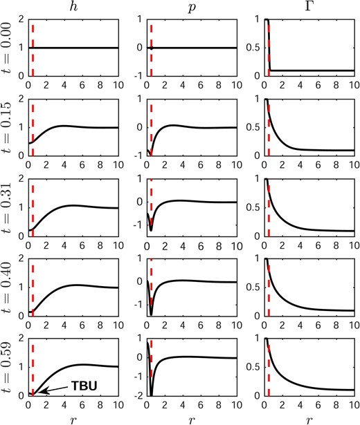
Dynamics of aqueous layer thickness for a spot glob. From left to right: aqueous layer thickness h, pressure p and surfactant concentration |$\varGamma$|⁠. The glob size R_I = 0.5 and TBU occurs at t = 0.59 s, when evaporation is not included. The vertical dashed line represents the glob edge at R_I.

A significant depression of the tear/air interface forms at 0.15 s as seen in the second row in the first column. Despite the fact that a low pressure area develops in this thin region, the resulting pressure gradient is insufficient to stop thinning under the glob. In this dimensional TBUT of 0.59 s, the aqueous layer thins from 3.5 μm–0.2 μm; the smaller value of 0.25 μm is the thickness which we defined as TBU. This TBUT is near unity non-dimensionally, which indicates that the timescales we chose work well. From this result, we conclude that the Marangoni flow dominates the thinning process in this case and leads to TBU in less than a second. In some in vivo observations with simultaneous fluorescence and lipid layer interferometry (King-Smith et al., 2013b), a dark spot in the fluorescence image, indicating a thin aqueous layer, forms under a corresponding area of extra lipid that appears bright in the lipid image. The dark spot in the aqueous layer forms by 0.14 s post blink, which is very rapid. The bright lipid glob spreads rapidly in this short post blink interval, but its center remains relatively bright and thus relatively thick. This experimental observation and the timescale of the dynamics correspond well with the model results.

Equations (3.23) and (3.32) imply that the strength of the Marangoni flow is directly proportional to the surfactant concentration gradient |$\partial_{r}\varGamma$|⁠. As the surfactant spreads out from the glob, the concentration gradient between the tear/glob and the tear/air interface decreases, which results in a weaker Marangoni flow. Meanwhile, the contribution to aqueous flow from capillarity, the pressure generated by surface tension and curvature of the tear/air interface, increases due to the deformation of the tear film. The Marangoni contribution to the flow is the divergent flow and the capillary contribution to the flow is the convergent flow. The two contributions to the flow have opposite directions and they compete with each other; different strengths of the initial Marangoni flow will lead to different outcomes of the dynamics. Fig. 3 shows that a strong initial Marangoni flow can lead to TBU in about 0.6 s.

Fig. 4 illustrates another case where the aqueous layer thins around the edge of the glob at short times, but then thickens at longer times. In the first column, the aqueous layer thickness h thins rapidly at the edge of glob at 2.94 s, the higher pressure surrounding the glob edge then pushes the water towards the thin region and subsequently heals the thin region at later times. In this case, the divergent flow from the Marangoni effect, though strong in the beginning, is insufficient to lead to TBU because the capillary contribution to flow (sometimes called healing flow, Peng et al., 2014) dominates the dynamics at later times.

Fig. 4.

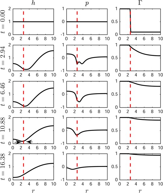
Dynamics of aqueous layer thickness with a spot glob of size R_I = 2.6. From left to right: aqueous layer thickness h, pressure p and surfactant concentration |$\varGamma$|⁠. Evaporation is not included. The vertical dashed line represents the edge of the glob. TBU would have occurred between the arrows, but instead h increased there.

Fig. 5 compares the Marangoni and capillary contributions to the aqueous flow for the same conditions as in Figs. 3 and 4. The left column shows that when the Marangoni effect dominates the capillary effect in the flow for a long enough time so that TBU occurs in 0.59 s (as in Fig. 3). In the right column, the Marangoni effect dominates the capillary effect only at very short times, then at later times the capillary effect dominates (as in Fig. 4). The result is that the net flux is positive (divergent) at very short times but switches to negative (convergent) fluxes at later times; TBU does not occur in this case. In vivo, experiments show that there are cases that show rapid initial thinning but then the thinning can reverse and TBU can be avoided; thus the model can behave similarly to experiments in this case as well.

Fig. 5.

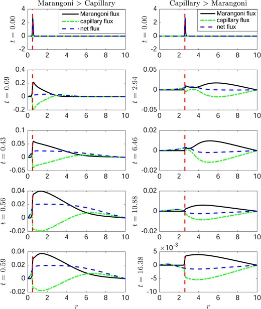
Comparison of the Marangoni and capillary contributions to flow in Figs. 3 and 4, with no evaporation (J = 0). The solid line, dash-dot line and dashed lines indicate the Marangoni term, the capillary term and net flow, respectively. The vertical dashed line represents the edge of glob. In the left column, outward (divergent) flow is rapid and leads to TBU at 0.59 s; the Marangoni effect dominates at all times, and we indicate this with the shorthand Marangoni>Capillary. The right column shows that capillarity dominates at later times and slows thinning enough to prevent TBU; we use the shorthand Marangoni<Capillary to label this case.

4.2. Dependence on surfactant concentration

As mentioned in Section 4.1, the strength of the Marangoni contribution is determined by |$\partial_{r}\varGamma$|⁠. Fig. 6(a) shows that larger initial surfactant concentration difference between that on the tear/glob interface and that on the tear/air interface |$[1-\varGamma(R_{L},0]$| leads to shorter TBUT. Larger concentration differences will induce a larger surfactant concentration gradients and thus a stronger Marangoni effect. When the initial surfactant concentration difference between the tear/glob and the tear/air interface is less than 0.5, the tangential flow is insufficient to lead to TBU. Whilst this is a simplified model of the tear film, this result suggests a threshold value below which variation of lipid layer will not cause TBU, and this could be a fruitful strategy to slow or reduce TBU in vivo. We discuss this point further below.

Fig. 6.

(a) Effect of initial surfactant concentration difference |$[1-\varGamma(R_{L},0]$| and (b) ||$\varDelta$|σ|₀ on TBUT when glob size is R_I = 0.5 without including evaporation. Here plot (b) is in loglog plot.

4.3. Representative change in surface tension

We varied the representative change in the surface tension ||$\varDelta$|σ|₀ from 10⁻⁴–10⁻³ N/m. Fig. 6(b) indicates that TBUT decreases by two orders of magnitude with increasing ||$\varDelta$|σ|₀. A larger representative change in surface tension results in a larger surface tension difference; thus the stronger Marangoni flow will then lead to TBU in a much shorter time. This effect of ||$\varDelta$|σ|₀ is encoded in the timescale, where t_s = σ₀dμ/[||$\varDelta$|σ|₀]².

4.4. Tear film evaporation rate

So far results for globs without evaporation have been shown. In this section, we discuss the effects of four different evaporation distributions as illustrated in Fig. 7(a); the equations used are given in Appendix  D, see (D.1–D.5). The evaporation distribution around globs is unknown and it is not known how to measure it at this time. We hypothesize different reasonable possibilities and explore the consequences of each. The evaporation distributions J(r, t) are functions based on four different hypotheses about the properties of the glob and surrounding tear film surface. Evaporation distribution (a) assumes that the glob is a good barrier to evaporation, its edge is a poor barrier and the tear/air interface is a uniformly good barrier. In this case, we assume that (i) J = 0 at the tear/glob interface; (ii) the evaporation rate increases significantly near the edge of the glob; (iii) outside of the edge of the glob, the tear/air interface has a low and uniform evaporation rate. The evaporation distribution (b) assumes that the glob is a better barrier to evaporation than tear/air interface, so there is a lower evaporation rate through the glob and a higher rate outside of it. The evaporation distribution (c) assumes a higher rate at the tear/glob interface but a lower rate on the tear/air interface. The evaporation distribution (d) assumes that the glob/tear and tear/air interfaces allow evaporation at the same rate and uses a uniformly distributed flux across entire domain.

Fig. 7.

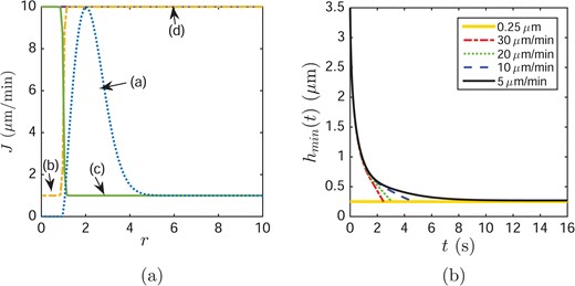
(a) Four different evaporation distributions with a maximum evaporation rate |$v_{\max } = 10\ \mu $|m/min and a minimum non-zero evaporation rate |$v_{\min } = 1\ \mu $|m/min. Only case a’ has a minimum evaporation rate of zero. (b) Effect of evaporation case a on TBUT. The horizontal line represents the TBU thickness 0.25 μm. The glob size is R_I = 1.5.

The dynamics of thinning are similar to previous cases shown; we summarize the results for TBUT using the different evaporation distributions and different maximum evaporation rates in Table 3. It is clear that in each column, an increasing evaporation rate leads to a shorter TBUT. Without evaporation (J = 0) the TBUT is 1.75 s, which is larger than all TBUT values in this table as expected. We conclude that evaporation is an additional driving mechanism that accelerates TBU. If we compare each column, the evaporation distribution (a) loses the least amount of water to the environment, with increasing amounts lost as one progresses from (b) to (d).

Table 3

TBUT results for spot globs with R_I = 1.5 using various evaporation distributions and maximum evaporation rates

|$v_{\max } (\mu $|m/min)	TBUT (s)
	(a)	(b)	(c)	(d)
5	1.68	1.51	1.48	1.38
10	1.60	1.38	1.32	1.21
20	1.44	1.21	1.13	1.01
30	1.30	1.10	1.01	0.90

Fig. 7(b) shows the minimum aqueous layer thickness as a function of time, |$h_{\min } (t) = \min _{r\in [0, R_{L}]} h(r,t)$|⁠, using the four different evaporation rates. The final values of these curves appear in Table 3, and the curves show similar trends. The horizontal line denotes the critical thickness defined as TBU (0.25 μm). The minimum tear film thickness decreases monotonically in these cases and higher evaporation rates cause faster thinning to TBU. Initially, the Marangoni stress dominates the loss of water, so the minimum thickness curves |$h_{\min }(t)$| are very close at small times even if the evaporation rate is significantly different. At later stages, the surfactant concentration gradient decreases and the different evaporation rates show more distinct dynamics, making the TBUT differences apparent.

4.5. Tear film thickness and glob size

Fig. 8(a) illustrates that by varying tear film thickness and glob size, our simulation gives TBUT in the range from 0.16–15 s. Since this model is specifically designed to explain glob-driven rapid TBU (TBUT < 3 or 4 s), the wide range of TBUT implies that other mechanisms lead to the larger TBUT. When the tear film thickness is fixed, TBUT initially decreases and then increases as the glob size increases. We call the glob radius that corresponds to the minimum TBUT the switching point. The switching points for the increasing tear film thicknesses shown are about 0.019 mm, 0.045 mm and 0.064 mm, respectively. The increasing value of the switching point is the result of increasing length scale; the length scale is proportional to the tear film thickness. As shown in Fig. 9, a smaller glob size corresponds a steeper tear film shape when TBU occurs. Since the capillary pressure is generated by the curvature of the tear film surface, for a glob size smaller than the switching point, the capillary pressure is larger and more difficult to overcome, which results in a longer TBUT when R_I < 0.25. When the glob size is much larger than the switching point (say R_I > 2.5), the shear stress remains unchanged, but there is more water covered by the glob. Thus, it takes longer to drag the water from under the glob and thus to reach TBU. For a fixed glob radius, a thinner tear film thickness corresponds to a shorter TBUT because there is less water under the glob.

Fig. 8.

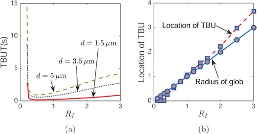
Effect of R_I on TBUT (a) and the location of TBU (b) with an evaporation distribution d; a uniformly high evaporation rate of 10 μm/min.

Fig. 9.

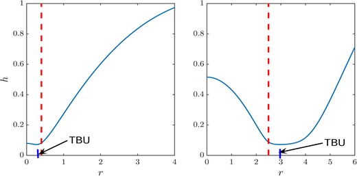
Tear film thickness profile for two different glob sizes for evaporation distribution (a) and a maximum evaporation rate |$v_{\max } = 10\ \mu $|m/min.

4.6. TBU position and glob size

The size of the glob not only affects TBUT but also changes the TBU position. Fig. 9 illustrates two cases: one where TBU happens under the glob when it is small, and the other where TBU happens at the edge (near R_I) when the glob is big. The vertical dashed line represents the edge of the glob. The plots show h(r, t) at TBU; and the short vertical line segment indicates the TBU position in each case. The location of TBU depends continuously on the glob size. Fig. 8(b) shows the relationship between TBU position and glob size. The line representing glob radius is shown for reference. When the TBU position is located below this line, the TBU is under the glob; otherwise it is outside the glob. When the glob radius is less than R_I = 0.9 (0.067 mm dimensionally when d = 3.5 μm), TBU happens under the glob, but happens outside for larger globs. When the glob is small, shear stress from the Marangoni effect can easily extract water from beneath the glob. However, when the glob is sufficiently large, the innermost water near the center of the glob is not affected strongly, and only water near the edge of the glob is dragged out by the Marangoni effect.

4.7. Streak TBU and comparison with spot TBU

The results from the previous Sections 4.1–4.6 showed results for (axisymmetric) spot TBU in cylindrical coordinates. We now turn to the (linear) streak TBU model in Cartesian coordinates given in Section 3. Overall, the dynamics of streak TBU are similar to those of spot TBU. We first consider results for |$J = v_{\max }$| and define the minimum aqueous thickness and surfactant concentration as the following equation (4.1):

\begin{align} h_{\min}(t) = \min_{r\in [0, R_{L}]} h(r,t), \quad \varGamma_{\min}(t) = \min_{r\in [0, R_{L}]} \varGamma(r,t). \end{align}

(4.1)

They are plotted as a function of time both streaks and spots in Fig. 10(a–b). One can see that spot TBU occurs more quickly than streak TBU for equal sizes (R_I = X_I). The spot TBU may be more rapid because the surfactant redistributes more rapidly for streaks compared to spots. Fig. 10(b) shows that this is the case; this is because the surfactant diffuses into a diverging (wider) area in the spot case as opposed to a constant width in the streak case. Because a greater surfactant concentration difference between the glob and the surrounding tear film remains for a longer time for spots, spots continue to drive a stronger Marangoni flow away from the glob as time progresses as shown in Fig. 6(a).

Fig. 10.

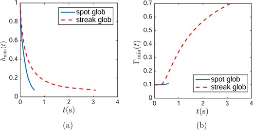
Dynamics of minimum thickness (a) and minimum surfactant concentration (b) when the streak and glob have the same size R_I = X_I = 0.5 with an evaporation distribution a and a maximum evaporation rate |$v_{\max } = 10\ \mu $|m/min.

We now consider evaporation with the streak model. Table 4 indicates that evaporation accelerates TBU because an increasing evaporation rate decreases TBUT. If we compare Tables 4 and 3, we observe in Table 3 that tears are dragged out more slowly in the streak glob than in the spot glob. Fig. 11(a) shows that when the streak is wider than X_I ≈ 0.7 ( 0.052 mm) for d = 3.5 μm), the thinnest tear film is found outside of glob. However, when the streak is narrower than that, the thinnest tear film is found inside the glob. Turning to the effect of tear film thickness d, with all other parameters the same, a thinner tear film decreases TBUT because there is less water under the glob; results are shown in Fig. 11(b). The increasing glob size first decreases TBUT, but then increases it. The switching point is where the minimum TBUT occurs for each thickness. For the streak globs, the switching points are, respectively for the increasing tear film thicknesses shown, |$X^{\prime }_{i}=0.0064$| mm, 0.0148 mm and 0.0212 mm. These switching points are significantly smaller than for spots as seen in Section 4.5.

Table 4

TBUT when glob streak has X_I = 1.5 with various evaporation fluxes and maximum evaporation rates

|$v_{\max }$| (μm/min )	TBUT (s)
	(a)	(b)	(c)	(d)
5	No TBU	5.58	4.86	4.21
10	4.69	3.76	3.27	2.83
20	3.08	2.61	2.22	1.94
30	2.44	2.11	1.78	1.56

Fig. 11.

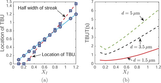
Effect of glob size on the location of TBU (a) and TBUT (b) with an evaporation d and maximum evaporation rate 10 μm/min.

5. Discussion

In this work, we studied models that simulate the fluid dynamics of the tear film driven by the presence of a single glob in the lipid layer. The model simplified the glob to a localized area of fixed and elevated concentration of insoluble surfactant that was hypothesized to correspond to polar lipids in the tear film. The model successfully captured the rapid thinning driven by a glob. The increased concentration of polar lipid spread out rapidly from the glob to the surrounding tear film which was initially at lower concentration. That concentration difference drives strong tangential flow and leads to TBU for globs that are not too small.

In order to match the timescale of the rapid thinning, we chose the velocity and length scales so that that Marangoni and capillary effects were both important and balanced; the timescale followed from that choice. As a consequence, with appropriate glob size, TBU can occur in under a second in the model. We view this as post facto justification for these choices. In addition, due to the comparable size of the two contributions to the flow, the tear film can behave differently for different size globs. It is found that the Marangoni contribution always dominates the capillary (pressure) contribution early in the computations. We observe TBU only when the Marangoni contribution to the flow is stronger for the entire computation. If tear film thinning is not fast enough, and the capillary contribution becomes stronger than the Marangoni contribution, then the divergent flow gives way to the convergent flow; the flow that thickens the film overcomes the flows that thins the film. Thus, in those cases, there won’t be rapid TBU, and there may be no TBU at all without substantial evaporation. Phenomena like these have been observed in some clinical observations, where relatively dark regions appear in fluorescence images but then they appear to brighten and heal (Braun et al., 2015). We showed results for both cases in Figs. 3 and 4. However, when glob size is as small as 0.037 mm, TBUT can be as long as 15 s. In that case, the Marangoni contribution is not the core mechanism because it is too weak to rapidly overcome the capillary pressure gradient of the small glob and TBU takes longer.

King-Smith et al. (2011) showed a large variety of structures of the lipid layer. Most of them contain different sizes of bright spots. Our model indicates that globs that are too small or too large won’t cause rapid thinning. TBU will only occur in under a second when the glob size is around the size of the switching point. Non-dimensionally, all switching points for streaks were about X_I = 0.2 and for spots were about R_I = 0.4. Because this was true for different d, this shows that our choice of length scales captures the point where the rapid thinning is most likely to occur. Most parameters in our model will affect the value of the switching point, including tear film thickness, the representative change of surface tension and the difference of lipid concentration. These quantities are difficult to measure accurately using current clinical techniques and are likely to vary from person to person. Thus, the model can provide a trend of how glob size affects TBU time and location, but the exact value of switching point will vary dependent on these parameters. Data from clinical experiments which record TBUT and corresponding glob size needed in order to validate this prediction. To the best of our knowledge, these data are not published.

Images from simultaneous aqueous layer fluorescence and TFLL interferometry are shown in Fig. 4 of (King-Smith et al., 2013b); these images are broadly consistent with our findings about glob size and position of TBU. In that figure, the upper images showed that a thinner aqueous layer occurred rapidly (about 0.12 s) under an area of thicker lipid. The lower images in that figure show that 3.6 s later the darkest fluorescence regions that remained after TBU occurred at the edges of the larger thick lipid spots. Our results in Figs. 8(b) and 11(a) agree with observation in both the upper and lower parts of their Fig. 4; (King-Smith et al., 2013b); we predict that small globs have TBU beneath the glob, whilst larger globs have TBU near their edges. Our model did not compute past the onset of TBU, so we were not able to compute beyond initial TBUT to produce images like those in the bottom part of their Fig. 4 (King-Smith et al., 2013b).

The important consequences of Marangoni flows seen here support the results in previous work even if those models may be exploring different phenomena. Jones et al. (2006) and Aydemir et al. (2010) simulated the tear film formation during the opening phase and subsequent tangential flows driven by polar lipid concentration gradients during the interblink. Zubkov et al. (2012) studied the consequences of complete blink cycles in a model that induced an insoluble surfactant and osmolarity; strong effects were observed there as well. Siddique & Braun (2015) investigated the effect of the Marangoni effect and a hypothesized dependence of evaporation rate on surfactant concentration for a model that replaced the TFLL with an insoluble surfactant layer. That model also observed important consequences from the Marangoni effect, but the model did not produce TBU from evaporation after spreading a localized increase in initial surfactant concentration. A key difference in this article is that the glob is at fixed concentration and location, so that the Marangoni effect continues to drive flow toward TBU provided that the glob is not too small. Bilayer models for the tear film (Bruna & Breward, 2014) also observed strong effects from the presence of an insoluble surfactant representing polar lipids.

We tested four different distributions of evaporation, and the results show that evaporation speeds up TBU. However, it does not have a strong effect on the dynamics of TBU and TBUT in this model. As shown in Fig. 7(b) the Marangoni contribution is typically so strong that no significant difference is observed in the first 2 s for evaporation rate from 5--20 μm/min. In this case, where the Marangoni effect leads to TBU in about 1 s or less, evaporation does not have enough time to significantly thin the tear film. Therefore, even though evaporation is a core mechanism in many dry eye cases (Kimball et al., 2010), it is not most important factor in the glob-driven rapid TBU that we study here. Our unpublished results also show that, in this case, evaporation is too slow to significantly increase osmolarity for the short TBUTs we considered. We note that this model and rapid thinning due to globs is a subset of observed TBU and that further research is needed to better understand its role in ocular surface phenomena and diseases such as DES. Either low or high levels of lipid secretion are known to occur in meibomian gland disease (MGD), which is a subtype of dry eye (Nelson et al., 2011).

There are other viewpoints on rapid TBU. Yokoi & Georgiev (2013b) discussed an alternative view; they suggest that rapid TBU can be classified based on the observed shape. They hypothesize that streak TBU is due to the Marangoni effect but spot breakup is the result of dewetting of defective patches of the corneal surface. They use their ideas to base individual treatment plans for DES. The dewetting mechanism appears to provide a good explanation of rapid TBU if it appears in a fixed position during different interblink periods (King-Smith et al., 2017). However, Fig. 1 shows that breakup can happen in different positions after each blink, and lipid spreading may be detected; in those cases, divergent flow driven by the Marangoni effect may be a better explanation for the images shown in this article and some others (King-Smith et al., 2013b,a).

These results strongly suggest that the quality of the lipid layer plays an important role in rapid thinning and uniform thickness is the key to a healthy lipid layer. Alterations in the normal lipid composition are associated with MGD (Shine & McCulley, 1998; McCulley & Shine, 2001; Shine & McCulley, 2003) and may be a factor in causing that type of dry eye (Nelson et al., 2011). Devising treatments based on altering these meibomian gland lipids may provide a promising avenue of treatment for some dry eye patients. The lipid-containing eye drops are also suggested as a potential treatment, cause it can improve the uniform thickness of the tear lipid layer (Geerling et al., 2011).

6. Conclusion and future work

We verified the hypothesis that Marangoni flow can be a physically reasonable explanation for streak and spot TBU that happens rapidly during an interblink. The polar lipid (surfactant) has a very strong initial gradient that drives a strong divergent flow outward from the glob because of the Marangoni effect, and this helps cause rapid outward spreading of the surfactant along the tear/air interface outside of the glob. When the tear/air interface deforms because of this flow, a pressure gradient contribution from capillarity is generated i.e. generally in the opposite direction. The two contributions compete with each other. When and whether TBU happens depends on which flow contribution is dominant at later times. The model show us that, if appropriate parameters are chosen (glob size, tear film thickness, etc), the Marangoni contribution to the flow can dominate and lead to TBU. With the help of evaporation, TBU can occur more quickly in some situations.

Our streak and spot models made similar predictions. Firstly, larger differences in polar lipid concentration between the tear/glob and tear/air interfaces lead to shorter TBUTs. This is consistent with the expectation that a healthy lipid layer is more uniform that a defective one. Secondly, when the representative change of surface tension (stronger Marangoni effect) is larger, the TBUT is shorter. Thirdly, rapid thinning is only related to glob size around the switching point defined as the minimum TBUT for each curve in Figs. 8(a) and 11(b). Globs which are too large or too small will increase the TBUT. Fourthly, small globs have the water drained from underneath creating TBU there, whereas large globs lead to TBU at their edges. The glob size affects the location of the resultant TBU. Lastly, including evaporation with the Marangoni effect can slightly speed up TBU but was typically is not very important in rapid TBU. The Marangoni contribution to flow dominates evaporation in the first second or so of the simulation, corresponding to the time post blink.

When we compared the 1D streak model with the axisymmetric spot model, there was one main difference. The results showed that the polar lipid concentration difference across the domain decreased over time for both models; but for spots, this decrease happened slowly compared to streaks. Thus, the Marangoni effect continues to drive a stronger outward flow in the aqueous layer, and this results in a shorter TBUT for spots with all other parameters equal.

The results of the model seem promising and suggest directions for future research for both the tear film and for mathematical modelling. We note that this model is based on greatly simplified physical assumptions. One assumption we made is that glob has a higher surfactant concentration, rather than greater thickness of the in vivo tear film lipid layer. We also assume that the glob has a fixed surfactant concentration, which in some cases is certainly changed by the flow in the tear film. Lastly, we assumed different evaporation profiles in our model that were different plausible distributions with respect to the lipid layer.

To be more realistic, a bilayer model can be developed to include the dynamics of a non-polar lipid layer i.e. anterior to the aqueous layer; a model with evaporation rates that depend on the thickness of a dynamic non-polar lipid layer has been published (Bruna & Breward, 2014). Our group has recently extended that model to fit measured thinning rates (Nichols et al., 2005; King-Smith et al., 2010) and use it to study TBU driven by increased evaporation through a hole in the non-polar lipid layer (as well as other cases). Both in the model and experiment, evaporative TBU takes 10 s to a minute or more, and causes hyperosmolarity in the TBU region (Liu et al., 2009; Peng et al., 2014; Braun et al., 2015, 2017). In contrast, the rapid TBU results that we compute are not expected to have elevated osmolarity in the TBU region, because there is insufficient time to lose water to the environment and thereby increase the osmolarity.

Our models here have limited TBU to simple streak or spot shapes; however, in many cases globs have irregular shapes. Extending our model to 2D irregular glob shapes would be an improvement. Adding osmosis and fluorescein transport can help study the effect rapid thinning has on the corneal surface, and for detailed comparison with fluorescence experiments. A simplified evaporative TBU model found some unexpected results for fluorescence imaging of streak and spot TBU (Braun et al., 2017), and we expect interesting results for quantitative interpretation in the rapid TBU case as well.

Finally, we hope that these results and predictions will help identify hypotheses and measurement quantities for in vivo experiments.

Funding

This work is funded by NSF (grant 1412085 to R.B.) and NIH (grant 1R01EY021794 to C.B. and grant R01EY17951 (to P.E.K.-S.). The content is solely the responsibility of the authors and does not necessarily represent the official views of the NSF or the NIH.

Appendix

A. Dimensional equations

We have listed dimensionless equations with only leading-order terms for the 1D streak and axisymmetric models in Section 3. In the following appendix we provide details about the dimensional equations.

The 1D streak model uses Cartesian coordinates, whilst the axisymmetric spot models uses cylindrical coordinates.

Inside the aqueous layer, we have (1) mass conservation and (2) momentum conservation:

\begin{equation} {\hskip-10pt}\nabla^{\prime} \cdot \mathbf{u}^{\prime} =0, \end{equation}

(A.1)

\begin{align} \rho \left (\partial_{t^{\prime}} \mathbf{u}^{\prime} + \mathbf{u}^{\prime}\cdot \nabla^{\prime} \mathbf{u}^{\prime} \right ) = -\nabla^{\prime} p ^{\prime} + \mu \nabla^{^{\prime}2} \mathbf{u}^{\prime}. \end{align}

(A.2)

At the corneal surface z′ = 0, we assume a no-slip boundary condition and also neglect the osmotic flow, since it is measured a weak flow (Nichols et al., 2005):

\begin{align} \mathbf{u}^{\prime} = 0. \end{align}

(A.3)

At the free surface z′ = h′, the kinematic boundary condition (A.4) implies that the evaporation flux is the only flow throughout this surface. The normal stress balance (A.5) at both tear/glob and tear/air interfaces takes into consideration the effects of surface tension and van der Waals dispersion forces:

\begin{align} J^{\prime} = \rho \left( \mathbf{u}^{\prime} - \mathbf{u}_{I}^{\prime}\right)\cdot \mathbf{n}^{\prime}, \end{align}

(A.4)

\begin{equation} {\hskip-63pt}-p_{v}^{\prime} - \mathbf{n}^{\prime} \cdot \boldsymbol{T} \cdot \mathbf{n}^{\prime} = \sigma_{0} \nabla^{\prime} \cdot \mathbf{n}^{\prime} - \frac{A^{\ast}}{h^{{\prime}3}}. \end{equation}

(A.5)

Here |$\mathbf{u}_{I}^{\prime }$| is the interface velocity, n′ is normal vector to the interface and T is the Newtonian stress tensor. Their definitions are the same as in Winter et al. (2010).

The glob is assumed to have different compositions at each of the interfaces. At the tear/glob interface |$\left (0,X_{I}^{\prime }\right )$|⁠, we assume a no-slip boundary condition (A.6) and a fixed surfactant concentration (A.7). We neglect the reduction of surfactant concentration on the glob since the tear film thins rapidly and TBU occurs quickly and faster than a blink cycle. These assumptions give:

\begin{equation} {\hskip-5pt}u^{\prime} = 0, \end{equation}

(A.6)

\begin{align} \varGamma^{\prime} = \varGamma_{0}. \end{align}

(A.7)

However, at the tear/air interface |$X_{I}^{\prime }<x<X_{L}^{\prime }$|⁠, the spreading glob increases the surfactant concentration and affects the tangential stress by changing the surface tension. Thus, we assume a tangential stress balance (A.8) and conservation of surfactant (A.9) at the tear/air interface:

\begin{align} \mathbf{t}^{\prime} \cdot \boldsymbol{T}\cdot \mathbf{n}^{\prime} = \partial_{S} \sigma = \mathbf{t}^{\prime} \cdot \nabla \sigma = \mathbf{t}^{\prime} \cdot \nabla \left [\sigma^{\prime}_{0} - \left | \partial_{\Gamma} \sigma \right |_{0} \left(\varGamma^{\prime} - \varGamma_{0}\right) \right ], \end{align}

(A.8)

\begin{equation} {\hskip-56pt}\partial_{t^{\prime}} \varGamma^{\prime} + \nabla_{s}^{\prime} \cdot (\varGamma^{\prime} \boldsymbol{u}^{\prime}) = D_{s} \nabla_{s}^{^{\prime}2} \varGamma^{\prime}. \end{equation}

(A.9)

Here t′ is the normal vector to the interface and |$\nabla _{s}^{\prime }$| is the surface operator which can be found in Slattery et al. (2007).

B. Dimensionless equations for 1D streak model

Our 1D streak model is built in Cartesian coordinates, where u′ = (u′, w′). Using the scaling in Section 3, we have the following dimensionless equations.

Inside the aqueous layer, 0 < z < h, 0 < x < X_L, conservation in mass and momentum is governed by the Navier Stokes equations:

\begin{equation} {\hskip-25pt}\partial_{x} u + \partial_{z} w = 0, \end{equation}

(B.1)

\begin{equation} {\hskip-8pt}\varepsilon^{2} Re (\partial_{t} u + u \partial_{x} u + w\partial_{z} u) = -\partial_{x} p + \varepsilon^{2} {\partial_{x}^{2}} u + {\partial_{z}^{2}} u, \end{equation}

(B.2)

\begin{align} \varepsilon^{4} Re (\partial_{t} w + u \partial_{x} w + w \partial_{z} w) = -\partial_{z} p +\varepsilon^{4} {\partial_{x}^{2}} w + \varepsilon^{2}{\partial_{z}^{2}} w. \end{align}

(B.3)

At the corneal surface z = 0, 0 < x < X_L, there’s no slip and no osmotic flow,

\begin{align} u(x,0,t) =w(x,0,t) = 0. \end{align}

(B.4)

At the free surface z = h, 0 < x < X_L, using the kinematic condition, the evaporation flux is

\begin{align} J = \frac{w - u\partial_{x} h - \partial_{t} h}{\sqrt{1+\varepsilon^{2} (\partial_{x} h)^{2}}}, \end{align}

(B.5)

while the normal stress balance is

\begin{align} p - p_{v} - \frac{2\varepsilon^{2}}{1+\varepsilon^{2} (\partial_{x} h)^{2}}\left[\varepsilon^{2}( \partial_{x} h)^{2} \partial_{x} u - \partial_{x} h \partial_{y} u + \varepsilon^{2} \partial_{x} h \partial_{x} w + \partial_{y} w\right] = \frac{ -S{\partial_{x}^{2}} h}{\left(1 + \varepsilon^{2} (\partial_{x} h)^{2}\right)^{3/2}} - Ah^{-3} . \end{align}

(B.6)

At the tear/glob interface, z = h, 0 < x < X_I, we have a no-slip and fixed surfactant concentration conditions

\begin{align} u = 0,\qquad \Gamma = 1 \; . \end{align}

(B.7)

At the tear/air interface, z = h, X_I < x < X_L, we have a tangential stress balance and conservation of surfactant concentration:

\begin{equation} \frac{(\partial_{z} u + \varepsilon \partial_{x} w)\left(1 - (\varepsilon \partial_{x} h)^{2}\right) + 2\varepsilon(\varepsilon \partial_{x} h)^{2} (\partial_{z} w - \partial_{x} u )}{1+\varepsilon^{2} (\partial_{x} h)^{2}} = \frac{-M\partial_{x} \varGamma }{ \left(1 + (\varepsilon \partial_{x} h)^{2}\right)^{1/2}}, \end{equation}

(B.8)

\begin{equation} {\hskip10pt}\varGamma_{t} + \frac{\partial_{x} (\varGamma u ) + \varepsilon^{2} \partial_{x} ( \partial_{x} (\varGamma w) )}{1+\varepsilon^{2}( \partial_{x} h)^{2}} =\textrm{Pe}_{s}^{-1}\frac{\partial_{x} \left ( \frac{\partial_{x} \varGamma }{1 + \varepsilon^{2} (\partial_{x} h)^{2}} \right )+ \varepsilon\partial_{x} h \partial_{x} \left ( \frac{\partial_{x} h \partial_{x}\varGamma}{1 + \varepsilon^{2} (\partial_{x} h)^{2}}\right ) }{1 + \varepsilon^{2} (\partial_{x} h)^{2}} . \end{equation}

(B.9)

Since the surface velocity is defined as |$\mathbf{u}^{\prime }_{s} = \mathbf{u}^{\prime } - (\mathbf{u}^{\prime }\cdot \mathbf{n}^{\prime })\mathbf{n}^{\prime }$|⁠, the dimensionless surface velocity is as follows:

\begin{align} \left( u +\varepsilon^{2}w \partial_{x} h, \varepsilon^{3} w (\partial_{x} h)^{2} + \varepsilon u \partial_{x} h\right)\Big/\left[1+\varepsilon^{2} (\partial_{x} h)^{2}\right]. \end{align}

(B.10)

If take only leading order terms, we get that the surface velocity is approximately equal to flow velocity at the corneal surface |$\mathbf{u}^{\prime }_{s} \approx (u,0) $|⁠. For convenience of interpretation, we write the u in (13) as u_s.

C. Axisymmetric spot model derivation

The spot model uses axisymmetric cylindrical coordinates. Let the dimensional velocity in axisymmetric coordinates be denoted as |$\mathbf{u}^{\prime }= \left (u^{\prime }_{r^{\prime }}, u^{\prime }_{z^{\prime }}\right )$|⁠. We choose a similar scaling as in the 1D streak model, as given in Section 3.

C.1 Dimensionless equations

The dimensionless equations for the conservation of mass and momentum are as follows:

\begin{equation} {\hskip-118pt}\frac{1}{r} \frac{\partial}{\partial r} (r u_{r}) + \frac{\partial u_{z}}{\partial z} =0, \end{equation}

(C.1)

\begin{align} \varepsilon^{2}\textrm{Re} \left( \partial_{t} u_{r} + u_{r} \partial_{r} u_{r} + \partial_{z} u_{r} \right) =- \partial_{r} p + \varepsilon^{2} \frac{1}{r} \frac{\partial}{\partial r} \left ( r \frac{\partial}{\partial r}u_{r}\right ) + \varepsilon^{2} \frac{u}{r^{2}} + {\partial_{z}^{2}} u_{r} \, \end{align}

(C.2)

\begin{equation} {\hskip-25pt}\varepsilon^{4}\textrm{Re} (\partial_{t} u_{z} + u_{r} \partial_{r} u_{z} + u_{z} \partial_{z} u_{z}) = -\partial_{z} p + \varepsilon^{4} \frac{1}{r} \frac{\partial}{\partial r}\left (r\frac{\partial}{\partial r} u_{z} \right ) + \varepsilon^{2} {\partial_{z}^{2}} u_{z}\ . \end{equation}

(C.3)

At corneal surface z = 0, 0 < r < R_L, we have no-slip boundary conditions for the radial and vertical component of the velocity,

\begin{align} u_{r}(r,0,t) = u_{z} (r,0,t) = 0. \end{align}

(C.4)

Kinematic condition and normal stress balance condition at the free surface z = h, 0 < r < R_L are

\begin{equation} {\hskip170pt}J = \frac{-u_{r} \partial_{r} h + u_{z} - \partial_{t} h}{\sqrt{1 + \varepsilon^{2} (\partial_{r} h)^{2}}}, \end{equation}

(C.5)

\begin{align} p-p_{v} - \frac{2\varepsilon^{4} (\partial_{r} h)^{2} \partial_{r} u_{r} - 2\varepsilon^{2} \partial_{r} h (\partial_{z} u_{r} + \varepsilon^{2} \partial_{r} u_{z}) + 2\varepsilon^{3} \partial_{z} u_{z}}{1+\varepsilon^{2} (\partial_{r} h)^{2}} = -S\frac{1}{r} \partial_{r} \left ( \frac{r\partial_{r} h}{\sqrt{1 + \varepsilon^{2} (\partial_{r} h)^{2}}}\right )-Ah^{-3} \; . \end{align}

(C.6)

At the tear/glob interface, z = h, 0 < r < R_I, we have the same conditions as in the 1D streak model

\begin{align} u_{r} = 0, \quad \varGamma = 1. \end{align}

(C.7)

At the tear/air interface, z = h, R_I < r < R_L, we satisfy a tangential stress balance and conservation of surfactant:

\begin{equation} {\hskip-80pt}\frac{\left(1-\varepsilon^{2}(\partial_{r} h)^{2} \right)\left(\varepsilon^{2} \partial_{r} u_{z} + \partial_{z} u_{r}\right) + 2\varepsilon^{2} \partial_{r} h (\partial_{z} u_{z} -\partial_{r} u_{r})}{1 + \varepsilon^{2}(\partial_{r} h)^{2}} = -M \frac{\partial_{r} \varGamma }{\sqrt{1 + \varepsilon^{2} (\partial_{r} h)^{2}}} \; , \end{equation}

(C.8)

\begin{align} \partial_{t} \varGamma + \frac{\partial_{r} (\varGamma u_{r}) + \varepsilon^{2} \partial_{r} h \partial_{r} (\varGamma u_{z})}{1+\varepsilon^{2} (\partial_{r} h)^{2}} + \frac{\varGamma u_{r}}{r} = \textrm{Pe}_{s}^{-1} \frac{\partial_{r} \left ( \frac{\partial_{r} \varGamma}{1 + \varepsilon^{2} (\partial_{r} h)^{2}}\right ) + \frac{\varGamma_{r}}{r}+ \varepsilon^{2} \partial_{r} h \partial_{r} \left (\frac{\partial_{r} h \partial_{r} \varGamma}{1+\varepsilon^{2} (\partial_{r} h)^{2}} \right ) }{1 +\varepsilon^{2} (\partial_{r} h)^{2} } \; . \end{align}

(C.9)

C.2 Leading order terms of dimensionless spot model

Let ε = 0 so we keep only the leading-order terms, then, our spot model simplifies to the following equations. Inside the aqueous layer 0 < z < h, 0 < r < R_L, the pressure gradient is independent of the vertical component and depends on the radial component of velocity:

\begin{equation} {\hskip-20pt}\frac{1}{r} \frac{\partial}{\partial r} (r u_{r}) + \frac{\partial u_{z}}{\partial z} =0, \end{equation}

(C.10)

\begin{align} \partial_{r} p =- {\partial_{z}^{2}} u_{r} \quad \textrm{and} \ \quad \partial_{z} p = 0. \end{align}

(C.11)

At corneal surface z = 0, 0 < r < R_L, we still have no-slip boundary conditions,

\begin{align} u_{r}(r,0,t)= u_{z}(r,0.t) =0, \end{align}

(C.12)

At the whole free surface (z = h, 0 < r < R_L), the kinematic boundary condition (C.13) and normal stress balance (C.14) simplify to

\begin{equation} {\hskip-35pt}\partial_{t} h + u_{r} \partial_{r} h - u_{z} = -J, \end{equation}

(C.13)

\begin{align} p - p_{v} = -S\frac{1}{r} \partial_{r} (r \partial_{r} h) - Ah^{-3}. \end{align}

(C.14)

At the tear/glob interface, z = h and 0 < r < R_I, we still have a no-slip BC and a fixed surfactant concentration

\begin{align} u_{r} = 0\, \quad \varGamma = 1. \end{align}

(C.15)

At the tear/air interface, z = h and R_I < r < R_L, we have that the radial component of velocity depends on the Marangoni flow and we have a surfactant concentration transport equation:

\begin{equation} {\hskip-103pt}\partial_{z} u_{r} = -M\partial_{r} \varGamma, \end{equation}

(C.16)

\begin{align} \partial_{t} \varGamma = \textrm{Pe}_{s}^{-1}\left [ \frac{1}{r}\partial_{r} (r \partial_{r} \varGamma)\right ] - \frac{1}{r}\partial_{r} (r \varGamma u_{r}). \end{align}

(C.17)

C.3 Blend boundary conditions

We use the following blend function:

\begin{align} B(r; R_{I}, R_{W}) = 0.5 + 0.5\tanh \left (\frac{r- R_{I}}{R_{w}} \right ), \end{align}

(C.18)

and to combine the boundary conditions at the tear/glob (C.19) and the tear/air interface (C.20):

\begin{equation} {\hskip-45pt}u_{r} (1-B) + (\partial_{z} u_{r} + M \partial_{r} \varGamma) B = 0, \end{equation}

(C.19)

\begin{align} \partial_{r} \varGamma = \left \{\textrm{Pe}_{s}^{-1}\left [ \frac{1}{r}\partial_{r} (r \partial_{r} \varGamma)\right ] - \frac{1}{r}\partial_{r} (r \varGamma u_{r}) \right \}B. \end{align}

(C.20)

The equations from (C.10) to (C.14) together with combined boundary conditions above (C.19) and (C.20) can be reduced into the systems of equations of Section 3.2.

D. Evaporation fluxes

We include four different distributions of evaporation.

• Case (a): Assume that the glob is a good barrier to evaporation, so that J = 0 across the tear/glob interface. However, the edge of glob is a poor barrier, the evaporation rate increases dramatically there. The tear/air interface behaves normally so that the evaporation rate is low and uniform.

  \begin{align} J (r)= a(1-v_{\min})(r-R_{I})e^{-(r- R_{I})^{2}/\left(2 {R_{W}^{2}} \right)}+v_{\min}\tanh\left(\frac{r-R_{I}}{ R_{W}}\right), \end{align}

  (D.1)

  where

  \begin{align} a = \frac{e^{1/2}[v_{\max}-v_{\min}\tanh(1)]}{(1-v_{\min}) R_{W}}. \end{align}

  (D.2)

  Here |$v_{\min }$| is the minimum evaporation rate, |$v_{\max }$| is maximum evaporation rate.

• Case (b): The glob is a better barrier than tear/air interface to evaporation. The evaporation rate is low on the glob but high at the tear/air interface:

  \begin{align} J(r) = v_{\min}\left [1- B(r) \right ]+v_{\max}B(r). \end{align}

  (D.3)

  Here B(r) = B(r; R_I, R_W) is the blend function (C.18).

• Case (c): The glob is a poorer barrier than mobile lipid layer to evaporation. The evaporation rate is high on the glob but low at the tear/air interface:

  \begin{align} J(r) = v_{\max}[1-B(r)] + v_{\min} B(r). \end{align}

  (D.4)
• Case (d): The different compositions of glob will not affect its ability to prevent evaporation, then we can assume a uniform evaporation across the entire domain:

  \begin{align} J(r) = v_{\max}. \end{align}

  (D.5)

E. Conservation of tears and increasing mass of surfactant

In this appendix, we provide evidence that our blend function introduces no significant new errors into the problem. First, we show that the use of a blend function for the aqueous film conserves the mass of fluid. Second, we use a model diffusion problem for the surfactant to show that the blended and non-blended versions converge for decreasing blend width X_W. This demonstrates that we can keep any new error introduced by the blend function small enough to approximate the desired problem.

E.1 Aqueous conservation

We now verify that our blend function is not causing any significant effect on mass conservation of aqueous fluid. Our blend function (3.16) is to help us combine different boundary conditions into a single expression so that we can have a single equation for each of the aqueous thickness and the surfactant concentration. To validate that using our blend functions preserves mass conservation, we eliminated evaporation by setting J = 0 and after solving for the PDEs numerically, we computed the integral of the aqueous layer thickness at each time (Trefethen, 2000; using Clenshaw--Curtis weights and nodes). As illustrated in Fig. E1(a), the error in the aqueous volume is quite small, which indicates that the blend function is acceptable for numerical computing. We do not aim to conserve the surfactant |$\varGamma$| in the same way. Our third assumption in Section 3 is that the glob has a fixed concentration, and so the glob acts as source that generates surfactant. Fig. E1(b) shows the resulting increase of surfactant over the domain for different glob sizes. Comparing the two curves in Fig. E1(b), we can see that the larger glob acts as a stronger source and generates more new lipid in the mobile part of the film surface.

Fig. E1.

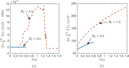
Plot of the difference between total volume at each time and the initial exact total volume |$ 2\pi \int _{0}^{10} h(r,t)r \ \textrm{d}r - 100\pi $| (a) and the total amount of lipid at each time |$2\pi \int _{0}^{10} \varGamma (r,t)r \ \textrm{d}r$| (b) when R_I = 0.5 or 1.5, and J = 0.

E.2 Surfactant model problem

Turning to the surfactant, the model we study in this article does converge to a single curve for the total amount of surfactant, |$I(t)=\int _{0}^{X_{L}}\varGamma (x,t)\textrm{ d}x$|⁠, as the width X_W of the blend function B is decreased (not shown). To show that there is vanishing difference between the blended and non-blended models, we study a simpler diffusion problem for |$\varGamma$|⁠. We demonstrate here that the blended and non-blended model diffusion problems converge to the same amount of |$\varGamma$| for X_W → 0 numerically. For the model problems, we consider

1. Problem 1:

   \begin{align} \partial_{t} \varGamma_{1} = B {\partial_{x}^{2}} \varGamma_{1} \quad 0<x<X_{L} . \end{align}

   (E.1)
2. Problem 2:

   \begin{equation} {\hskip-16pt}\varGamma_{2} = 1,\quad 0< x < X_{I}- \delta . \end{equation}

   (E.2)

   \begin{align} \partial_{t} \varGamma_{2} = {\partial_{x}^{2}} \varGamma_{2}, \quad X_{I} - \delta < x < X_{L} . \end{align}

   (E.3)

We are solving a blended diffusion in problem 1 with |$\varGamma \approx 1$| to the left of X_I, and diffusing for x > X_I, which mimics aspects of the problem of this article. Problem 2 solves a diffusion problem on X_I − δ < x < X_L, with constant |$\varGamma = 1$| to the left of this interval; no blending is performed. We choose an offset δ = 2X_W that makes the transitions of the initial conditions roughly the same width; the width decreases with X_W for both problems.

Fig. E2.

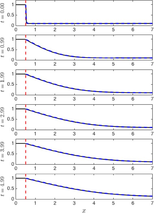
Plots of |$\varGamma_1$| (solid) and |$\varGamma_2$| (dashed) at several different times. The solutions are difficult to distinguish graphically except near X_I near t = 0.

Both problems share the following boundary conditions.

\begin{align} \partial_{x} \varGamma(0,t) = \partial_{x} \varGamma (X_{L}, t) = 0, \end{align}

(E.4)

though we use |$\varGamma$|(X_I − δ, t) = 1 for computing solutions to problem 2 on the interval where diffusion occurs. We choose initial conditions for |$\varGamma_1$| the same as in (28). For |$\varGamma_2(x,0)$| in X_I − δ < x < X_L, we choose

\begin{align} \varGamma_{2}(x,0) = \varGamma_{L} + (1-\varGamma_{L}) \exp [ -a (x-X_{I}+\delta)] \ . \end{align}

(E.5)

We choose the decay constant a as follows. We enforced equal initial total mass for both problems,

\begin{align} \int_{0}^{X_{L}} \varGamma_{1}(x,0) \textrm{ d}x - \int_{0}^{X_{L}} \varGamma_{2}(x,0) \textrm{ d}x =0; \end{align}

(E.6)

evaluating the integrals and simplifying yield the transcendental equation

\begin{align} a \delta - 1 + \exp \left[ -a(X_{L}-X_{I}+\delta)\right] =0\ . \end{align}

(E.7)

Solving for the positive value of a is straightforward given δ = 2X_W, X_L and X_I; we used fzero in Matlab. A sample computation is shown in Fig. E2; here X_w = 0.01, X_L = 10, X_I = 0.5 and a majority of the domain are shown at each time. The initial conditions for the blended case (problem 1, solid) and the non-blended case (problem 2, dashed) are close when considered pointwise, with minor differences around X_I. The solutions are difficult to distinguish graphically thereafter.

For a quantitative measure of conservation, we compute |I₁(t) − I₂(t)| where |$I_{1}(t)=\int _{0}^{X_{L}} \varGamma _{1}(x,t)\textrm{ d}x$| and |$I_{2}(t)=\int _{X_{I}-\delta }^{X_{L}} \varGamma _{2}(x,t)\textrm{ d}x+X_{I}-\delta $|⁠; these are the total amount of |$\varGamma_{i}$| for each problem i = 1, 2. For the same conditions X_w = 0.01, X_L = 10 and X_I = 0.5, the difference in mass between the two problems is shown in Fig. E3(a). The difference is zero initially by design; it then increases early and decreases at later times. The difference was never large in our computations.

Fig. E3.

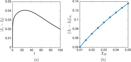
(a) The difference in total amount of surfactant between problems 1 and 2 as function of time. (b) The maximum difference in total |$\varGamma$| over time is plotted for different X_W. There appears to be roughly linear convergence to the same total |$\varGamma$| for the two problems.

It is important that the difference between the two problems decrease for decreasing blend function width; results for different X_W are shown in Fig. E3(b). The two problems appear to converge to the same total |$\varGamma$| at a roughly linear rate. This justifies our use of the blend function to approximate the non-blended problem.