Optimal modality selection in external beam radiotherapy

Abstract

The goal in external beam radiotherapy (EBRT) for cancer is to maximize damage to the tumour while limiting toxic effects on the organs-at-risk. EBRT can be delivered via different modalities such as photons, protons and neutrons. The choice of an optimal modality depends on the anatomy of the irradiated area and the relative physical and biological properties of the modalities under consideration. There is no single universally dominant modality. We present the first-ever mathematical formulation of the optimal modality selection problem. We show that this problem can be tackled by solving the Karush–Kuhn–Tucker conditions of optimality, which reduce to an analytically tractable quartic equation. We perform numerical experiments to gain insights into the effect of biological and physical properties on the choice of an optimal modality or combination of modalities.

multi-modality radiotherapy, nonlinear optimization, fractionation

1. Introduction

External beam radiotherapy (EBRT) uses high-energy, ionizing radiation generated outside the patients, e.g. by linear accelerators or cyclotrons, to kill cancerous tumour cells. Unfortunately, radiation also damages nearby organs-at-risk (OAR). Thus, the goal is to maximize the damage to the tumour while limiting below a tolerable level the toxic effects on the OAR. In an ongoing quest for attaining this goal, several modalities for delivering EBRT have been devised (Halperin, 2006; Schaue & Mcbride, 2015; Baumann et al., 2016). EBRT is most prevalent in the form of photon beam x-rays (Lawrence et al., 2008; Halperin et al., 2013). It is also administered using beams of charged particles such as protons (Schulz-Ertner et al., 2006; Grutters et al., 2010; Ramaekers et al., 2011; Loeffler & Durante, 2013; Tommsino et al., 2015). Heavier, carbon ions are emerging as yet another option for charged particle therapy (Ebner & Kamada, 2016; Schulz & Kagan, 2016). Among all patients receiving particle therapy by the end of 2013, 87.5% were treated with protons and 10.8% with carbon ions (Tommsino et al., 2015). Other rarer delivery mechanisms such as neutrons, pions, boron-neutron capture therapy and charged-nuclei therapy have also been investigated (Halperin, 2006; Rong & Welsh, 2010).

Different modalities can be compared, at least in theory, based on three criteria: biological behaviour, physical (dosimetric) characteristics and cost (Halperin, 2006; Peeters et al., 2010; Rong & Welsh, 2010; Mitin & Zietman, 2014). This paper focuses on the trade-offs introduced by biological and physical characteristics as described in the next two paragraphs. A cost-benefit analysis of different modalities would require entirely different techniques, and hence it is deferred to future research.

Differences in biological behaviour across modalities

Biological behaviour is comprised of two main items: relative biological effectiveness (RBE) and oxygen enhancement ratio (Halperin, 2006). RBE captures the fact that different modalities produce different levels of cell-damage for the same amount of physical radiation dose (measured in J/kg or Gy). Oxygen enhancement ratio is the ratio of radiation doses needed to produce the same level of tumour cell kill in poorly oxygenated conditions as in well-oxygenated conditions. This accounts for the observation that oxygen increases radiosensitivity of tumour cells. For example, neutrons have a higher RBE and a lower oxygen enhancement ratio than photons (Halperin, 2006; Rong & Welsh, 2010).

Differences in physical (dosimetric) characteristics across modalities

The main physical characteristic of a modality is its dose depth deposition profile (Halperin, 2006; Rong & Welsh, 2010; Mitin & Zietman, 2014). This profile describes the radiation dose deposited as a function of the distance travelled inside a medium. Photon x-rays deposit a high dose near the entry point and the dose then decreases with distance (Halperin et al., 2013). Protons exhibit a different profile. The deposited dose is roughly constant with distance from the entrance point; abruptly reaches a peak (called the Bragg peak) deeper inside the medium; and then falls sharply after the peak (Halperin, 2006; Rong & Welsh, 2010; Ebner & Kamada, 2016). Thus, by positioning the Bragg peak precisely in the cancerous region, a large dose differential between the tumour and the OAR can be attained. This in turn means that a large dose can be delivered to the tumour while still keeping the OAR dose within tolerable limits (Grutters et al., 2010). Carbon ions also exhibit a similar profile but with a slower post-peak drop in dose and have a higher RBE (Schulz-Ertner & Tsujii, 2007; Ebner & Kamada, 2016).

No universally superior modality

Each modality offers certain advantages and disadvantages with respect to the above two criteria (Rong & Welsh, 2010). For instance, neutrons are not superior to photons or to protons in terms of their dose deposition profiles, but have a much higher RBE. This high RBE does, however, imply that neutrons are highly toxic to both the tumours and the OAR (Halperin, 2006). The RBE of protons is only about 10% higher than photons (Paganetti et al., 2002; Paganetti & van Luijk, 2013; Paganetti, 2014), but protons have a much favourable dose deposition profile as explained above. One important disadvantage with protons is that it is difficult to precisely position the Bragg peak in the cancerous region owing to various uncertainties; thus the risk of a high OAR toxicity has to be carefully managed (Paganetti, 2012; Baumann et al., 2016). Treatment with protons and other charged particles is also currently much more expensive than photon therapy (Loeffler & Durante, 2013; Ramaekers et al., 2013). In addition, due to the longest history of using photons in cancer treatments, the most sophisticated ancillary systems are currently available for photon EBRT to aid precise localization of the tumours, e.g. image-guided radiotherapy.

No clear winner that dominates all other modalities in all three criteria has emerged thus far. This was summarized by Halperin (2006) a decade ago: ‘Neutrons, photons, pions, alpha particles, stripped nuclei, protons, and electrons vary in their biological, physical, and cost characteristics. None has yet met the test of being the generic ideal particle. Instead, each of these particles will probably offer advantages for particular histological types of cancer, at specific stages, in certain clinical conditions. An understanding of the biology of tumours should help to clarify the ideal particle for a clinical situation. Much of the history of the search for the ideal particle has yet to be created.’ A similar sentiment was reiterated by McDermott and by Schulz & Kagan in 2016, and by Baumann et al. in 2016. Missing a universally superior EBRT modality, some studies have considered combinations of two modalities (typically photons and protons) to leverage their physical and biological advantages (Yonemoto et al., 1997; Bertuzzi et al., 2001; Feuvret et al., 2007; Torres et al., 2009; DeLaney, 2009, 2011; DeLaney et al., 2014; Maio et al., 2015; Chen et al., 2016).

Lack of randomized clinical trials

One hurdle in deciding an ideal modality or a combination of two modalities is that no randomized clinical trial results comparing outcomes of different modalities are currently available. For instance, the prevalent EBRT modality for prostate cancer is still photons, but it is also where proton therapy has been used most widely (Mitin & Zietman, 2014 reported that 70% of patients who received proton therapy by 2014 had prostate cancer). Nevertheless, in January 2016, Schiller et al. (2016) stated, ‘There are still no completed randomized trials comparing proton-beam therapy with photon-beam therapy in men with clinically localized prostate cancer.’ A year later, this has not changed. Indeed, in February 2017, Tyson et al. (2017) commented, ‘Although there is some evidence that novel radiation therapies may improve the dose distribution with higher doses delivered locally to the tumor thereby preserving surrounding healthy tissues, these assertions remain unproven in studies to date ... . ... there are no randomized clinical trials comparing proton therapy to conventional radiation therapy.’ This lack of randomized clinical trials extends to other cancers where the use of proton beams is rarer than prostate. For example, after a retrospective comparison between photons and protons for 243,822 non-small cell lung cancer patients in the National Cancer Database (photons: 243,474; protons: 348), Higgins et al. (2017) stated in January 2017 that ‘further validation in the randomized setting is needed.’ Similarly, Ramaekers et al. (2011) performed a meta-analysis of 86 observational studies (74 photon, 5 carbon ion and 7 proton) on head-and-neck cancers and concluded in 2010: ‘several reviews indicated that based on clinical evidence it remains unclear, mainly because of the absence of randomized trials, whether particle therapy is superior over radiotherapy with photons ... .’ A similar observation was repeated four years later by Ahn et al. (2014). This situation might not significantly change in the near future, given the ethical, financial and logistical difficulties involved in the design of randomized clinical trials (Goitein & Cox, 2008; Morgan, 2008; van Loon et al., 2012; Dekker et al., 2014; Lambin et al., 2017).

Further challenges posed by fractionation

The selection of an appropriate modality is further complicated because radiotherapy is typically administered in multiple treatment sessions over several weeks. This is called fractionation. Healthy tissues possess better damage-repair capabilities than tumours (Withers, 1985; Hall & Giaccia, 2005). Fractionation thus gives healthy tissue time to recover between treatment sessions. For any single radiation modality, the optimal number of fractions and the corresponding dose in each fraction depend on (i) the relative difference between the tumour’s and the healthy tissue’s biological response to that modality, (ii) the dose deposition profile of that modality with respect to the anatomy of the irradiated area and (iii) the tumour proliferation rate. The trade-offs in determining an optimal number of fractions and doses have been studied over the past several decades mainly for photon therapy (Rockwell, 1988; Fowler, 1990, 2001, 2007, 2008; Fowler & Ritter, 1995; Jones et al., 1995; Horiot et al., 1997, 1992; Fu et al., 2000; Garden, 2001; Armpilia et al., 2004; Ahamad et al., 2005; Trotti et al., 2005; Yang & Xing, 2005; Ho et al., 2009; Marzi et al., 2009; Arcangeli et al., 2010; Kader et al., 2011; Keller et al., 2012; Mizuta et al., 2012; Bertuzzi et al., 2013; Unkelbach et al., 2013a, b; Bortfeld et al., 2015; Saberian et al., 2015, 2016, 2017; Badri et al., 2016).

Literature on mathematical optimization models for single-modality fractionation

Given the aforementioned difficulties in designing randomized clinical trials, many of the above studies formulate and solve theoretical optimization models of the single modality fractionation problem to guide decisions. These formulations are rooted in the following linear-quadratic (LQ) model of tumour’s response to radiation dose (Hall & Giaccia, 2005; O’Rourke et al., 2009):

\begin{equation} f=e^{-N(\alpha^{\tau} d+\beta^{\tau} d^2)+\pi(N)}. \end{equation}

(1)

Here, |$f$| is the fraction of tumour cells that survive; |$N$| is the number of treatment sessions; |$d$| is the dose per session; |$\pi (N)$| models tumour proliferation as a function of |$N$|⁠; and |$\alpha ^{\tau }, \beta ^{\tau }$| are tumour-specific parameters. The goal is to minimize the fraction of surviving tumour cells subject to upper limit constraints on the biological effect (BE) (Hall & Giaccia, 2005) on OAR. In the LQ framework, BE is defined by the expression

\begin{equation} N\left(\alpha^{\phi} (sd)+\beta^{\phi} (sd)^2\right). \end{equation}

(2)

Here, |$\alpha ^{\phi }, \beta ^{\phi }$| are OAR-specific parameters, and |$s$| is the so-called sparing factor, which equals the ratio of doses delivered to the OAR and tumour. This results in a non-convex quadratically constrained quadratic programming problem. Such problems in general belong to the class NP-hard (Luo et al., 2010). Existing work on solving this theoretical single modality fractionation model thus includes various heuristic and exact solution methods that exploit the structure of its formulation. For example, a closed-form solution is derived in Bortfeld et al. (2015), Fowler (2008), Fowler & Ritter (1995), Jones et al. (1995), Mizuta et al. (2012), Saberian et al. (2016) and Unkelbach et al. (2013a) for the case of a single OAR; a simulated annealing heuristic is used in Yang & Xing (2005) and Karush–Kuhn–Tucker (KKT) conditions are employed in Bertuzzi et al. (2013) for an extension with two OAR; we showed in Saberian et al. (2016) that an exact solution can be derived for the case of multiple OAR using KKT conditions when problem parameters are ordered a certain way; it is shown in Badri et al. (2016) and Saberian et al. (2015) that the problem with multiple OAR can be solved to optimality by reformulating it as a two-variable linear program.

There is a different stream of literature, where single-modality dosing decisions are made by combining the LQ model with differential equations that describe tumour growth. Analytical solution of those formulations is typically not possible, and numerical simulations are often performed to compare select few dosing strategies (Enderling et al., 2006, 2007, 2010; Corwin et al., 2013; Poleszczuk et al., 2013; Powathil et al., 2013, 2007; Lewin et al., 2018).

When two modalities are available, additional trade-offs arising from their RBE and dose deposition profiles need to be considered. To the best of our knowledge, no existing mathematical work has modelled this fractionation problem with two modalities.

Contributions of this paper

The objective of this paper is to propose a novel, mathematical framework to systematically investigate the selection of optimal modalities in radiotherapy, balancing the trade-off in the biological and physical (dosimetrical) characteristics unique to each radiation modality currently available in practice. The rest of this paper is organized as follows. In Section 2 of this paper, we provide a mathematical formulation of the fractionation problem with two modalities, where the goal is to find an optimal number of treatment sessions and the corresponding dose per session for each modality. We show that KKT conditions for this formulation can be tackled by solving an analytically tractable quartic equation. In Section 3, we perform sensitivity analyses to gain insight into the effect of problem parameters on the choice of optimal modalities. These parameters characterize biological and physical behaviours of the two modalities under consideration. In one set of sensitivity analyses (Section 3.1), we consider two modalities that have comparable physical characteristics but distinct biological characteristics. One example of this could be photons and neutrons. In the second set of sensitivity analyses (Section 3.2), we consider two modalities that have comparable biological characteristics but distinct physical characteristics. One example of this could be photons and protons. This ‘one-at-a-time’ manner of performing sensitivity analyses facilitates the interpretation of results, although it is not a requirement of our mathematical model itself. Finally, although our initial formulation focuses on the single OAR case for ease of exposition, we briefly describe how our KKT approach can be extended to multiple OAR in Section 4. We conclude in that section by outlining opportunities for future work.

2. Problem formulation and solution

In this section, we provide a formulation of the fractionation problem with two modalities using the LQ dose-response model. We use notation that is standard in the single modality fractionation literature, except that, in our case, modalities are indexed by |$i=1,2$|⁠. Modality |$1$| is assumed to be the ‘conventional’ modality such as photon EBRT. Let |$N_i$| denote the number of treatment sessions administered (once daily) with modality |$i$|⁠. Similarly, let |$d_i$| denote the tumour-dose in each one of the |$N_i$| sessions for modality |$i$|⁠. Moreover, |$\alpha ^{\tau }_i, \beta ^{\tau }_i$| denote the parameters of the tumour’s LQ dose-response model for modality |$i$|⁠. Notation |$\pi (N_1+N_2)$| represents tumour proliferation over a treatment course that includes |$N_1+N_2$| sessions. We employ a particular form for the proliferation function |$\pi (\cdot )$| in our numerical results later; in this section, we simply emphasize that it depends on the length of the treatment course as is standard in the literature. Let |$s_i$| denote the OAR’s sparing factor for modality |$i$|⁠. That is, the dose to OAR |$i$| equals |$s_i d_i$|⁠. A procedure for calculating sparing factors is described in Saberian et al. (2016). Let |$\alpha ^{\phi }_i, \beta ^{\phi }_i$| denote the OAR’s LQ dose-response parameters for modality |$i$|⁠. Suppose that the OAR is known to tolerate a dose of |$d_{\textrm{conv}}$| per session when administered using the conventional modality |$1$| in |$N_{\textrm{conv}}$| sessions. Then, the BE of this conventional treatment plan equals |$B=N_{\textrm{conv}}\alpha ^{\phi }_1 d_{\textrm{conv}}+N_{\textrm{conv}}\beta ^{\phi }_1(d_{\textrm{conv}})^2$|⁠. As in Saberian et al. (2017), |$N_{\max }$| is a constant, which is interpreted as a loose upper bound on the total number of sessions that is logistically viable in practice irrespective of the selected modality. Using a large value for this constant (say 100 or 200 sessions) ensures that all relevant combinations of |$N_1$| and |$N_2$| will be evaluated by our solution method. The thought process in our stylized formulation is that |$s_1, s_2$| characterize the physical properties of the two modalities, whereas |$\alpha $|⁠, |$\beta $| and |$\tau $| correspond to the biological ones.

We pursue the standard approach of minimizing the fraction of surviving tumour cells subject to the constraint that the BE of the treatment plan is no more than the conventional BE that the OAR is known to tolerate. This yields the formulation

\begin{align} (P)\ \min\limits_{N_1,d_1,N_2,d_2} e^{-N_1\alpha^{\tau}_1 d_1-N_1\beta^{\tau}_1 (d_1)^2-N_2\alpha^{\tau}_2 d_2-N_2\beta^{\tau}_2 (d_2)^2+\pi(N_1+N_2)} \end{align}

(3)

\begin{align} N_1\left[\alpha^{\phi}_1(s_1 d_1)+\beta^{\phi}_1 (s_1d_1)^2\right]+N_2\left[\alpha^{\phi}_2 (s_2 d_2)+\beta^{\phi}_2(s_2d_2)^2\right] &\leq B, \end{align}

(4)

\begin{align} \qquad \qquad \qquad \qquad \qquad \qquad \qquad \qquad \qquad \qquad \qquad \quad d_1 &\geq 0, \end{align}

(5)

\begin{align} \qquad \qquad \qquad \qquad \qquad \qquad \qquad \qquad \qquad \qquad d_2 &\geq 0, \end{align}

(6)

\begin{align}\qquad \qquad \qquad \qquad \qquad \qquad \qquad \qquad \qquad N_1+N_2&\leq N_{\max }, \end{align}

(7)

\begin{align} \qquad \qquad \qquad \qquad \qquad \qquad \qquad \qquad \qquad \qquad \qquad \qquad 0 \leq N_1\ &\textrm{integer}, \end{align}

(8)

\begin{align} \qquad \qquad \qquad \qquad \qquad \qquad \qquad \qquad \qquad \qquad \qquad \qquad 0 \leq N_2\ &\textrm{integer}. \end{align}

(9)

Note that the above formulation explicitly allows |$N_1=0$| or |$N_2=0$|⁠, which corresponds to the single modality case. It also allows other combinations where both |$N_1>0$| and |$N_2>0$|⁠, which corresponds to administering a combination of modalities as has been attempted in some clinical studies cited in Section 1 (Yonemoto et al., 1997; Bertuzzi et al., 2001; Feuvret et al., 2007; Torres et al., 2009; DeLaney, 2009, 2011; DeLaney et al., 2014; Maio et al., 2015; Chen et al., 2016). A benefit of this approach is that it exhaustively compares all such possibilities in one shot.

We now make a few observations about problem |$(P)$|⁠. It can be tackled by first solving the indexed group of problems

\begin{align} \left(P\left(N_1,N_2\right)\right)\ \min\limits_{d_1,d_2} e^{-N_1\alpha^{\tau}_1 d_1-N_1\beta^{\tau}_1 (d_1)^2-N_2\alpha^{\tau}_2 d_2-N_2\beta^{\tau}_2 (d_2)^2+\pi(N_1+N_2)} \end{align}

(10)

\begin{align} N_1\left[\alpha^{\phi}_1 \left(s_1 d_1\right)+\beta^{\phi}_1 \left(s_1d_1\right)^2\right]+N_2 \left[\alpha^{\phi}_2 \left(s_2d_2\right)+\beta^{\phi}_2\left(s_2d_2\right)^2\right] &\leq B, \end{align}

(11)

\begin{align} \qquad \qquad \qquad \qquad \qquad \qquad \qquad \qquad \qquad \qquad \qquad d_1 &\geq 0, \end{align}

(12)

\begin{align}\qquad \qquad \qquad \qquad \qquad \qquad \qquad \qquad \qquad \qquad \qquad d_2 &\geq 0, \end{align}

(13)

for all non-negative integer pairs |$(N_1,N_2)$| such that |$0\leq N_1+N_2\leq N_{\max }$|⁠. In particular, let |$d^{\ast }_1(N_1,N_2)$| and |$d^{\ast }_2(N_1,N_2)$| denote optimal doses for modalities |$1,2$| in problem |$(P(N_1,N_2))$|⁠, respectively. Let |$F^{\ast }(N_1,N_2)$| denote the optimal objective value of problem |$(P(N_1,N_2))$|⁠. Then problem |$(P)$| can be solved by minimizing |$F^{\ast }(N_1,N_2)$| over all integer pairs |$(N_1,N_2)$| such that |$0\leq N_1+N_2\leq N_{\max }$|⁠. If the pair |$N^{\ast }_1, N^{\ast }_2$| is optimal for this problem, then the quadruple |$N^{\ast }_1, d^{\ast }_1(N^{\ast }_1,N^{\ast }_2), N^{\ast }_2, d^{\ast }_2(N^{\ast }_1,N^{\ast }_2)$| is optimal for problem |$(P)$|⁠. Since the exponential function is monotonic in its argument, minimizing the objective function in |$(P(N_1,N_2))$| is equivalent to minimizing |$- N_1\alpha ^{\tau }_1 d_1-N_1\beta ^{\tau }_1 (d_1)^2-N_2\alpha ^{\tau }_2 d_2-N_2\beta ^{\tau }_2 (d_2)^2+\pi (N_1+N_2)$|⁠. Further, since the pair |$N_1,N_2$| is fixed in problem |$ (P(N_1,N_2))$|⁠, the proliferation term |$\pi (N_1+N_2)$| is a constant that can be ignored without loss of optimality. Finally, the objective function is decreasing in |$d_1$| and |$d_2$| and the left-hand side of constraint (11) is increasing in |$d_1$| and |$d_2$|⁠. Thus, constraint (11) must be active at an optimal solution. In other words, solving |$(P(N_1,N_2))$| is equivalent to solving

\begin{align} \left(Q\left(N_1,N_2\right)\right)\ \min\limits_{d_1,d_2} -\left(N_1\alpha^{\tau}_1 d_1+N_1\beta^{\tau}_1 \left(d_1\right)^2+N_2\alpha^{\tau}_2 d_2+N_2\beta^{\tau}_2 \left(d_2\right)^2\right) \end{align}

(14)

\begin{align} N_1\left[\alpha^{\phi}_1 \left(s_1d_1\right)+\beta^{\phi}_1 \left(s_1d_1\right)^2\right]+N_2\left[\alpha^{\phi}_2 \left(s_2 d_2\right)+\beta^{\phi}_2\left(s_2d_2\right)^2\right] &=B, \end{align}

(15)

\begin{align}\qquad \qquad \qquad \qquad \qquad \qquad \qquad \qquad \qquad \qquad \qquad d_1 &\geq 0, \end{align}

(16)

\begin{align}\qquad \qquad \qquad \qquad \qquad \qquad \qquad \qquad \qquad \qquad \qquad d_2 &\geq 0. \end{align}

(17)

An exact solution method based on KKT conditions for |$(Q(N_1,N_2))$| is developed in Appendix  A. This method is applied to perform numerical sensitivity analyses in the next section.

3. Numerical results

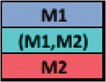
Let |$M_1$| denote a conventional modality such as photon EBRT, and let |$M_2$| denote an alternative modality. Table 1 illustrates a legend for three colours that will be employed throughout this section to indicate the use of modalities |$M_1$|⁠, |$(M_1,M_2)$| mixture and |$M_2$|⁠, respectively.

Table 1

Legend of colours showing three different modality choices.

Our numerical results are categorized into two parts that are presented in Sections 3.1 and 3.2, respectively. Section 3.1 investigates the trade-offs between |$M_1$| and a biologically superior |$M_2$|⁠. Section 3.2 studies the trade-offs between |$M_1$| and a physically superior |$M_2$|⁠. Recall that biological and physical are the two main characteristics of a modality as described in Section 1. As stated in Section 1, we pursue this one-at-a-time method of performing sensitivity analyses because it facilitates interpretation of our results. In both Sections 3.1 and 3.2, these trade-offs are explored for different values of a biological parameter |$r=\alpha ^{\phi }_2/\alpha ^{\tau }_2$| that we introduce in this paper. The thought process behind this parameter is as follows. A biologically superior modality will inflict a higher damage on both the tumour and the OAR. The ratio |$r$| attempts to capture the differential in the damage to the tumour and the OAR. As |$r$| increases, the damage to the OAR relative to the damage to the tumour using |$M_2$| increases, when all other things are equal. Thus, |$M_2$| becomes less desirable as |$r$| increases. For the conventional modality |$M_1$|⁠, we used |$s_1=1$| as the base value of physical characteristics throughout this paper. Also, for |$M_1$|⁠, we used |$\alpha ^{\tau }_1/\beta ^{\tau }_1 = 10$| Gy, |$\alpha ^{\phi }_1/\beta ^{\phi }_1 = 2$| Gy and the OAR tolerance was assumed to be |$N_{\textrm{conv}}d_{\textrm{conv}}=50$| Gy delivered in |$N_{\textrm{conv}}=25$| fractions (Hall & Giaccia, 2005; Marks et al., 2010). Table 2 shows other specific parameter values for |$M_1$|⁠. Similarly, |$\beta ^{\phi }_2$| was fixed at |$0.175$||$\textrm{Gy}^{-2}$| and |$\beta ^{\tau }_2$| was fixed at |$0.035$||$\textrm{Gy}^{-2}$| throughout this paper. These values are standard in the clinical literature (Hall & Giaccia, 2005; Fowler, 2007, 2008; Marks et al., 2010), and yield |$B=35$| as the right-hand side of constraint (4).

Table 2

Parameters for the conventional modality |$M_1$|⁠.

|$\alpha ^{\tau }_1 = 0.35$| Gy|$^{-1}$|	|$\beta ^{\tau }_1 = 0.035$| Gy|$^{-2}$|
|$\alpha ^{\phi }_1 = 0.35$| Gy|$^{-1}$|	|$\beta ^{\phi }_1 = 0.175$| Gy|$^{-2}$|

For the tumour repopulation term |$\pi (N_1+N_2)$| in the expression for BE in the objective function of problem |$(P)$|⁠, we used

\begin{align} \pi\left(N_1+ N_2\right) = \frac{\left[(N_1+N_2) - 1-T_{\textrm{lag}}\right]^+ \ln 2}{T_d}, \end{align}

(18)

where |$T_d$| and |$T_{\textrm{lag}}$| are tumour doubling time and lag time, respectively; and |$[\cdot ]^+ = \max (\cdot , 0)$|⁠. This functional form for tumour repopulation is common in the literature (Hall & Giaccia, 2005; Fowler, 2007), and it assumes that tumour repopulation does not start until |$T_{\textrm{lag}}$| days after treatment begins.

In this study, we present results with |$T_d=3$| days and |$T_{\textrm{lag}}=0$| day as representative values since qualitative trends in our results were invariant with respect to these numbers. We fixed |$N_{\max }$| at 200 days throughout.

Our evaluation criterion equals the ratio of surviving cells attained by an optimal modality relative to that attained by the conventional modality. We assume that ‘standard practice’ delivers radiotherapy using conventional modality (⁠|$M_1$|⁠) only for 25 fractions, i.e. |$N_{\textrm{conv}}=25$|⁠. We compute the ratio of surviving cells in three ways. First, we fix the number of treatment sessions to |$N_{\textrm{conv}}=25$|⁠, and compute the ratio of surviving cells attained by an optimal modality relative to that attained by the conventional modality. This amounts to comparing the effect of optimizing the choice of modality (without optimizing the number of sessions) against standard practice. Second, we re-compute this ratio, but this time by also optimizing the number of sessions in the numerator. This amounts to comparing the effect of solving problem |$(P)$| against standard practice. Finally, we calculate this ratio again, but this time by also optimizing the number of sessions in the denominator.

3.1 Biologically superior modality |$M_2$| combined with conventional modality |$M_1$|

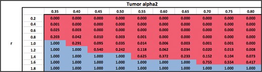
In this section, we investigate the case where |$M_2$| is biologically superior to |$M_1$| (when |$r=1$|⁠) as characterized by higher values of |$\alpha ^{\tau }_2$| in the range 0.35–0.8 Gy|$^{-1}$|⁠. The physical characteristics of |$M_2$| are assumed to be similar to |$M_1$| and hence |$s_2$| is fixed at |$1$| in this section. For example, this section therefore studies trade-offs between conventional photon EBRT and neutrons. Results are summarized in Tables 3–6.

Table 3

Ratio of surviving cells attained by using an optimal modality (or combination) with |$N_{\rm conv}$| = 25 fractions, relative to using |$M_1$| with |$N_{\rm conv} =$|25 fractions.

Table 4

Optimal number of fractions and optimal modality.

Table 5

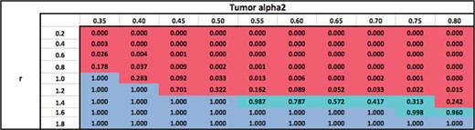
Ratio of surviving cells attained by using an optimal modality with an optimal number of fractions, relative to using |$M_1$| with |$N_{\rm conv}$| = 25 fractions.

Table 3 shows the ratio of surviving cells when an optimal modality (or combination) is used with the total number of fractions fixed at |$N_{\textrm{conv}}=25$|⁠, relative to the standard practice of using |$M_1$| with |$N_{\textrm{conv}}=25$| fractions. The table shows that for a fixed |$\alpha ^{\tau }_2$|⁠, the optimal modality switches from |$M_2$| to |$M_1$| as |$r$| increases since the relative damage to the OAR from |$M_2$| becomes larger, making |$M_2$| less desirable. For a fixed |$r$|⁠, the optimal modality switches from |$M_1$| to |$M_2$| as |$\alpha ^{\tau }_2$| increases since the biological power of |$M_2$| becomes larger. Therefore, for sufficiently low fixed values of |$r$|⁠, i.e. when the damage to the OAR from |$M_2$| is relatively lower than the damage to the tumour, |$M_2$| dominates |$M_1$| for all values of |$\alpha ^{\tau }_2$| because of |$M_2$|’s superior biological power (⁠|$\alpha ^{\tau }_2> \alpha ^{\tau }_1$|⁠). Similarly, |$M_1$| dominates |$M_2$| for all values of |$\alpha ^{\tau }_2$| for sufficiently high values of |$r$| due to the high toxicity to the OAR from |$M_2$|⁠. The switch from |$M_1$| to |$M_2$| occurs at higher values of |$\alpha ^{\tau }_2$| as |$r$| increases. This is because, the biological power of |$M_2$|⁠, i.e. |$\alpha ^{\tau }_2$| has to be sufficiently high for that modality to become desirable despite its higher damage to the OAR (large |$r$|⁠). Similarly, the switch from |$M_2$| to |$M_1$| occurs at higher values of |$r$| as |$\alpha ^{\tau }_2$| increases. For each fixed value of |$\alpha ^{\tau }_2$|⁠, the surviving cell ratio is nondecreasing as |$r$| increases because |$M_2$| becomes less desirable. Similarly, for each fixed value of |$r$|⁠, the surviving cell ratio is nonincreasing as |$\alpha ^{\tau }_2$| increases because |$M_2$| becomes more desirable.

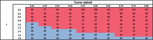
Table 4 shows optimal modalities and the optimal number of fractions obtained by solving problem |$(P)$| (in contrast with Table 3 wherein the number of fractions is not optimized). The qualitative trends in the choice of optimal modality are identical to that in Table 3 as expected. Moreover, for each fixed |$\alpha ^{\tau }_2$|⁠, the optimal number of fractions is nonincreasing as |$r$| increases when |$M_2$| is the optimal modality. This may be because as |$M_2$| damages the OAR more and more relative to the tumour, prolonged fractionation is less desirable. For each fixed |$r$|⁠, the optimal number of fractions follows a more complicated trend as |$\alpha ^{\tau }_2$| increases when |$M_2$| is the optimal modality. For some values of |$r$|⁠, it first increases and then decreases, whereas for other values of |$r$| it decreases. The optimal number of fractions is independent of |$\alpha ^{\tau }_2$| and |$r$| as expected, when |$M_1$| is the optimal modality.

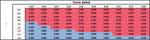
Table 5 shows the ratio of surviving cells when an optimal modality is used with an optimal number of fractions, relative to the standard practice of using |$M_1$| with |$N_{\textrm{conv}}=25$| fractions (in contrast to Table 3 wherein the number of fractions is not optimized). As expected, the surviving cell ratios are lower in Table 5 than in Table 3. This is because (for the optimal modality) the number of fractions is optimized in Table 5 whereas it is fixed at |$N_{\textrm{conv}}=25$| in Table 3. All other qualitative trends regarding the choice of optimal modalities in Table 5 are identical to those in Table 3.

Finally, Table 6 shows the ratio of surviving cells when an optimal modality is used with an optimal number of fractions, relative to using |$M_1$| with a number of fractions that is optimal for |$M_1$| (contrast this with Tables 5 and 3). As expected, the surviving cell ratios are higher in Table 6 than in Table 5. This is because the number of fractions with |$M_1$| is optimized in Table 6 but not in Table 5. All other qualitative trends regarding the choice of optimal modalities in Table 6 are identical to those in Table 5.

3.2 Physically superior modality |$M_2$| combined with conventional modality |$M_1$|

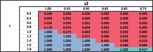
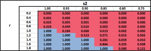
In this section, we investigate the case where |$M_2$| is physically superior to |$M_1$| as characterized by |$s_2 < s_1=1$| (recall that we fix |$s_1=1$| in all numerical experiments). The biological characteristics of |$M_2$| are assumed to be similar to |$M_1$| when |$r=1$|⁠. For example, this section therefore studies trade-offs between conventional photon EBRT and protons. Results are summarized in Tables 7–10 over the ranges of 0.2–1.8 for |$r$|⁠, and 1.0–0.75 for |$s_2$|⁠.

Table 6

Ratio of surviving cells attained by using an optimal modality with an optimal number of fractions, relative to using |$M_1$| only with a number of fractions that is optimal for |$M_1$|⁠.

Table 7

Ratio of surviving cells attained by using an optimal modality (or combination) with |$N_{\rm conv}$| = 25 fractions, relative to using |$M_1$| with |$N_{\rm conv}$| = 25 fractions.

Table 8

Optimal number of fractions and optimal modality.

Table 9

Ratio of surviving cells attained by using an optimal modality with an optimal number of fractions, relative to using |$M_1$| with |$N_{\rm conv}$| = 25 fractions.

Table 10

Ratio of surviving cells attained by using an optimal modality with an optimal number of fractions, relative to using |$M_1$| only with a number of fractions that is optimal for |$M_1$|⁠.

Table 7 shows the ratio of surviving cells when an optimal modality (or combination) is used with the total number of fractions fixed at |$N_{\textrm{conv}}=25$|⁠, relative to the standard practice of using |$M_1$| with |$N_{\textrm{conv}}=25$| fractions. The table shows that for a fixed |$s_2$|⁠, the optimal modality switches from |$M_2$| to |$M_1$| as |$r$| increases because the relative damage to the OAR from |$M_2$| becomes larger, making |$M_2$| less desirable. For a fixed |$r$|⁠, the optimal modality switches from |$M_1$| to |$M_2$| because |$M_2$| delivers less dose to the OAR (superior physical characteristics). Therefore, for sufficiently low fixed values of |$r$|⁠, |$M_2$| dominates |$M_1$| for all values of |$s_2$| because |$M_2$| inflicts only a small damage to the OAR compared to the tumour. Similarly, for sufficiently high values of |$r$|⁠, |$M_1$| or |$(M_1,M_2)$| dominates |$M_2$| for all values of |$s_2$|⁠. The switch from |$M_1$| to |$M_2$| occurs at lower values of |$s_2$| as |$r$| increases. Similarly, the switch from |$M_2$| to |$M_1$| occurs at higher values of |$r$| as |$s_2$| decreases. For each fixed value of |$s_2$|⁠, the surviving cell ratio is nondecreasing as |$r$| increases because |$M_2$| becomes less desirable. Similarly, for each fixed value of |$r$|⁠, the surviving cell ratio is nonincreasing as |$s_2$| decreases because |$M_2$| becomes more desirable. The logic behind all these trends is qualitatively similar to that in Table 3.

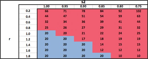
Table 8 shows optimal modalities and the optimal number of fractions obtained by solving problem |$(P)$| (in contrast with Table 7 wherein the number of fractions is not optimized). The qualitative trends in the choice of optimal modality are identical to that in Table 7 as expected. Moreover, for each fixed |$s_2$|⁠, the optimal number of fractions is nonincreasing as |$r$| increases when |$M_2$| is the optimal modality. Again, this may be because as |$M_2$| damages the OAR more and more relative to the tumour, prolonged fractionation is less desirable. For each fixed |$r$|⁠, the optimal number of fractions seems to be nondecreasing as |$s_2$| decreases when |$M_2$| is the optimal modality. This may be because the damage to the OAR decreases as |$s_2$| decreases and hence prolonged fractionation could be beneficial. The optimal number of fractions is independent of |$s_2$| and |$r$| as expected, when |$M_1$| is the optimal modality.

Table 9 shows the ratio of surviving cells when an optimal modality is used with an optimal number of fractions, relative to using |$M_1$| with |$N_{\textrm{conv}}=25$| fractions (in contrast to Table 7 wherein the number of fractions is not optimized). As expected, the surviving cell ratios are lower in Table 9 than in Table 7. This is because (for the optimal modality) the number of fractions is optimized in Table 9 whereas it is fixed at |$N_{\textrm{conv}}=25$| in Table 7. All other qualitative trends regarding the choice of optimal modalities in Table 9 are identical to those in Table 7.

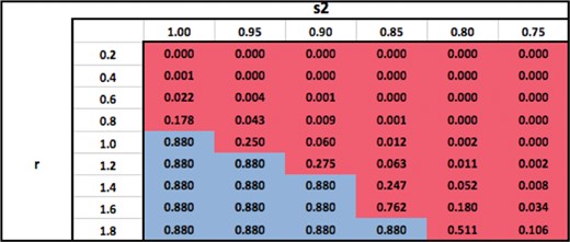
Finally, Table 10 shows the ratio of surviving cells when an optimal modality is used with an optimal number of fractions, relative to using |$M_1$| with a number of fractions that is optimal with |$M_1$| (contrast this with Tables 9 and 7). As expected, the surviving cell ratios are higher in Table 10 than in Table 9. This is because the number of fractions with |$M_1$| is optimized in Table 10 but not in Table 9. All other qualitative trends regarding the choice of optimal modalities in Table 10 are identical to those in Table 9.

4. Conclusions

We presented the first-ever mathematical formulation of the optimal fractionation problem with two modalities under the LQ dose-response model. We showed that KKT conditions for this formulation can be tackled by solving a quartic equation. Our numerical experiments explored the effect of varying, in a one-at-a-time manner, parameters that characterize physical and biological properties of the two modalities. The results of these experiments were consistent with clinical intuition. This at least partially validates our formulation and solution methodology, and therefore, the proposed framework may provide optimal solutions for more complex scenarios where clinical intuition is less obvious.

Although we focused on the case of a single OAR for simplicity, our methodology can be easily extended to multiple OAR. To see this, consider a problem with |$M$| OAR. Its formulation would include |$M$| constraints similar to (4). At least one of these constraints must be active at an optimal solution. So, if there is exactly one constraint active at an optimal solution, we need to consider |$M$| different possibilities. Furthermore, at most two active constraints are needed to uniquely determine a |$(d_{1},d_{2})$| combination. There are |$M\atop 2$| ways in which we can have two active constraints. These observations suggest that a problem with |$M$| OAR can be solved by (i) solving |$M$| problems with one OAR each via the method presented in this paper, (ii) solving |$M\atop 2$| quartic equations to uniquely identify additional candidate |$(d_1,d_2)$| pairs and (iii) identifying and comparing all feasible |$(d_1,d_2)$| pairs derived from steps (i) and (ii).

The framework proposed in this paper can be further extended to clinically relevant scenarios. For example, uncertainty in various problem parameters was not explicitly incorporated into our formulation, although it is of special interest in some modalities such as protons. Effects of uncertainty were only indirectly studied via sensitivity analyses. Formulations that explicitly include uncertainty in parameters may provide an interesting direction for future research.

Acknowledgements

This research was funded in part by the National Science Foundation through grant 1560476.

Appendix. A. Technical details about solution method for |$Q(N_1,N_2)$|

There are three possibilities: |$d_1>0, d_2=0$|⁠; |$d_1=0, d_2>0$|⁠; and |$d_1>0, d_2>0$|⁠. In the first two cases, the problem reduces to a single modality problem, which can be solved simply by solving a quadratic equation derived from constraint (15). Specifically, in the first case, a candidate |$d_1$| is given by

\begin{equation} d_1=\frac{-N_1s_1\alpha_1^{\phi}+\sqrt{N^2_1s^2_1\big(\alpha_1^{\phi}\big)^2+4N_1\beta^{\phi}_1s^2_1B}}{2N_1\beta^{\phi}_1 (s_1)^2}. \end{equation}

(A.1)

In the second case, a candidate |$d_2$| is given by

\begin{equation} d_2=\frac{-N_2s_2\alpha_2^{\phi}+\sqrt{N^2_2s^2_2\big(\alpha_2^{\phi}\big)^2+4N_2\beta^{\phi}_2s^2_2B}}{2N_2\beta^{\phi}_2 (s_2)^2}. \end{equation}

(A.2)

In order to explore the third case, we attach Lagrange multipliers |$\lambda $|⁠, |$\mu _1$| and |$\mu _2$| with the three constraints (11)–(13), respectively. Then KKT conditions (see Equations (5.49) on page 243 of Boyd & Vandenberghe, 2004) for this problem can be written as |$\mu _1\geq 0$|⁠, |$\mu _2\geq 0$|⁠, |$\mu _1 d_1=0$|⁠, |$\mu _2 d_2=0$|⁠, |$d_1\geq 0$|⁠, |$d_2\geq 0$| and

\begin{align} N_1 s_1 \alpha^{\phi}_1 d_1+N_1 \beta^{\phi}_1 (s_1d_1)^2+N_2 s_2 \alpha^{\phi}_2 d_2+N_2 \beta^{\phi}_2 (s_2d_2)^2 &=B, \end{align}

(A.3)

\begin{align} \left[\begin{array}{@{}c@{}}-\mu_1\\-\mu_2\end{array}\right]+\lambda\left[\begin{array}{@{}c@{}}N_1s_1\alpha^{\phi}_1+2N_1\beta^{\phi}_1s^2_1d_1\\N_2s_2\alpha^{\phi}_2+2N_2\beta^{\phi}_2s^2_2d_2 \end{array}\right]=\left[\begin{array}{@{}c@{}} N_1\alpha^{\tau}_1+2N_1\beta^{\tau}_1 d_1\\ N_2\alpha^{\tau}_2+2N_2\beta^{\tau}_2 d_2\\ \end{array}\right]. \end{align}

(A.4)

Since |$d_1>0$| and |$d_2>0$|⁠, we know that |$\mu _1=\mu _2=0$|⁠. Substituting this into the system (A.4) of equations yields

\begin{align} d_1&=\frac{\lambda s_1\alpha^{\phi}_1-\alpha^{\tau}_1}{2\big(\beta^{\tau}_1-\lambda\beta^{\phi}_1s^2_1\big)}, \end{align}

(A.5)

\begin{align} d_2&=\frac{\lambda s_2\alpha^{\phi}_2-\alpha^{\tau}_2}{2\big(\beta^{\tau}_2-\lambda\beta^{\phi}_2s^2_2\big)}. \end{align}

(A.6)

Substituting this back into (A.3) yields the following quartic equation:

\begin{align} \nonumber \lambda^4&\left(-16B\big(\beta_1^{\phi}\big)^2\big(\beta_2^{\phi}\big)^2s^4_1s^4_2-4\big(\alpha_1^{\phi}\big)^2\beta_1^{\phi}\big(\beta_2^{\phi}\big)^2N_1s^4_1s^4_2-4\big(\alpha_2^{\phi}\big)^2\beta_2^{\phi}\big(\beta_1^{\phi}\big)^2N_2s^4_2s^4_1\right)\\\nonumber &+ \lambda^3\Big(32B\big(\beta_1^{\phi}\big)^2\beta_2^{\phi}\beta_2^{\tau} s^4_1s^2_2+16\big(\alpha_1^{\phi}\big)^2\beta_1^{\phi}\big(\beta_2^{\phi}\big)^2N_1s^4_1s^2_2-8\big(\alpha_1^{\phi}\big)^2\beta_1^{\phi}\beta_2^{\phi}\beta_2^{\tau} N_1s^4_1s^2_2\\ \nonumber &+8\big(\alpha_2^{\phi}\big)^2\big(\beta_1^{\phi}\big)^2\beta_2^{\tau} N_2s^4_1s^2_2+32B\beta_1^{\phi}\beta_1^{\tau}\big(\beta_2^{\phi}\big)^2s^2_1s^4_2+8\big(\alpha_1^{\phi}\big)^2\beta_1^{\tau}\big(\beta_2^{\phi}\big)^2N_1s^2_1s^4_2\\ \nonumber & \quad 16\big(\alpha_2^{\phi}\big)^2\big(\beta_1^{\phi}\big)^2\beta_2^{\phi} N_2s^2_1s^4_2-8\big(\alpha_2^{\phi}\big)^2\beta_1^{\phi}\beta_1^{\tau}\beta_2^{\phi} N_2s^2_1s^4_2\Big)\\ \nonumber &+ \lambda^2\Big(-16B\big(\beta_1^{\phi}\big)^2\big(\beta_2^{\tau}\big)^2s^4_1-8\big(\alpha_1^{\phi}\big)^2\beta_1^{\phi}\big(\beta_2^{\phi}\big)^2 N_1s^4_1+4\big(\alpha_1^{\phi}\big)^2\beta_1^{\phi}\big(\beta^{\tau}_2\big)^2N_1s^4_1\\ \nonumber &-8\alpha_2^{\phi}\alpha_2^{\tau}\big(\beta_1^{\phi}\big)^2\beta_2^{\tau} N_2 s^4_1s_2-64B\beta_1^{\phi}\beta_1^{\tau}\beta_2^{\phi} \beta_2^{\tau} s^2_1s^2_2-16\big(\alpha_1^{\phi}\big)^2 \beta_1^{\tau}\big(\beta_2^{\phi}\big)^2N_1s^2_1s^2_2\\ \nonumber &-16\big(\alpha_2^{\phi}\big)^2\big(\beta_1^{\phi}\big)^2 \beta^{\tau}_2N_2s^2_1s^2_2-16\alpha_1^{\phi}\alpha_1^{\tau}\beta_1^{\phi}\big(\beta_2^{\phi}\big)^2N_1s^3_1s^2_2+16\alpha_1^{\phi}\alpha_1^{\tau}\beta_1^{\phi}\beta_2^{\phi}\beta_2^{\tau} N_1s^3_1s^2_2\\ \nonumber &+4\big(\alpha_2^{\tau}\big)^2\big(\beta_1^{\phi}\big)^2\beta_2^{\phi} N_2s^4_1s^2_2-16\alpha_2^{\phi}\alpha_2^{\tau}\big(\beta_1^{\phi}\big)^2\beta_2^{\phi} N_2s^2_1s^3_2+16\alpha_2^{\phi}\alpha_2^{\tau}\beta_1^{\phi}\beta^{\tau}_1\beta_2^{\phi} N_2s^2_1s^3_2\\ \nonumber &-16B\big(\beta_1^{\tau}\big)^2\big(\beta_2^{\phi}\big)^2s^4_2-8\big(\alpha_2^{\phi}\big)^2\big(\beta_1^{\phi}\big)^2\beta_2^{\phi} N_2s^4_2+4\big(\alpha_2^{\phi}\big)^2\big(\beta_1^{\tau}\big)^2\beta_2^{\phi} N_2s^4_2\\ \nonumber &-8\alpha_1^{\phi}\alpha_1^{\tau}\beta_1^{\tau}\big(\beta_2^{\phi}\big)^2N_1s_1s^4_2+4\big(\alpha_1^{\tau}\big)^2\beta_1^{\phi}\big(\beta_2^{\phi}\big)^2N_1s^2_1s^4_2\Big)\\ \nonumber &+ \lambda\Big(32B\beta_1^{\phi}\beta_1^{\tau}\big(\beta_2^{\tau}\big)^2s^2_1+8\big(\alpha_1^{\phi}\big)^2\beta_1^{\tau}\big(\beta_2^{\phi}\big)^2N_1s^2_1+8\alpha_1^{\phi}\alpha_1^{\tau}\beta_1^{\phi}\big(\beta_2^{\phi}\big)^2N_1s^3_1\\ \nonumber &-8\alpha_1^{\phi}\alpha_1^{\tau}\beta_1^{\phi}\big(\beta_2^{\tau}\big)^2N_1s^3_1+16\alpha_2^{\phi}\alpha_2^{\tau}\big(\beta_1^{\phi}\big)^2 \beta_2^{\tau} N_2s^2_1S_2+32B\big(\beta_1^{\tau}\big)^2\beta_2^{\phi} \beta_2^{\tau} s^2_2\\ \nonumber &+ 8\big(\alpha_2^{\phi}\big)^2\big(\beta_1^{\phi}\big)^2\beta_2^{\tau} N_2s^2_2+16\alpha_1^{\phi}\alpha_1^{\tau}\beta_1^{\tau}\big(\beta_2^{\phi}\big)^2N_1s_1s^2_2-8\big(\alpha_1^{\tau}\big)^2\beta_1^{\phi}\beta_2^{\phi}\beta^{\tau}_2N_1s^2_1s^2_2\\ \nonumber &-8\big(\alpha_2^{\tau}\big)^2\beta_1^{\phi}\beta_1^{\tau}\beta_2^{\phi} N_2s^2_1s^2_2 +8\alpha_2^{\phi} \alpha_2^{\tau}\big(\beta_1^{\phi}\big)^2\beta_2^{\phi} N_2s^3_2-8\alpha_2^{\phi} \alpha_2^{\tau}\big(\beta_1^{\tau}\big)^2\beta_2^{\phi} N_2s^3_2\Big)\\ \nonumber &+ \Big(-16B\big(\beta_1^{\tau}\big)^2\big(\beta^{\tau}_2\big)^2-8\alpha_1^{\phi}\alpha_1^{\tau} \beta^{\tau}_1\big(\beta_2^{\phi}\big)^2 N_1s_1+4\big(\alpha_1^{\tau}\big)^2\beta_1^{\phi} \big(\beta_2^{\tau}\big)^2N_1s^2_1\\ \nonumber &-8\alpha_2^{\phi}\alpha_2^{\tau}\big(\beta_1^{\phi}\big)^2\beta^{\tau}_2N_2s_2+4\big(\alpha_2^{\tau}\big)^2\big(\beta_1^{\tau}\big)^2\beta_2^{\phi} N_2s^2_2\Big)=0. \end{align}

This quartic equation can be easily solved analytically or numerically. Its real roots can then be substituted back into (A.5) and (A.6) to obtain candidate solutions. After solving the quartic equation, there are four possible cases for each real root that need to be considered separately based on the form of (A.5) and (A.6). In particular, the cases evaluate whether or not the numerator and/or denominator in (A.5) and (A.6) are zero.

1. Denominator and numerator of (A.5) are zero: |$\lambda =\beta ^{\tau }_1/(\beta _1^{\phi } s_1^2)= \alpha ^{\tau }_1/(s_1\alpha _1^{\phi })$|⁠.

   • (a) Denominator of (A.6) is zero: |$\lambda =\beta ^{\tau }_2/(\beta _2^{\phi } s^2_2)$|⁠.

     • i. Numerator of (A.6) is zero: |$\lambda =\alpha ^{\tau }_2/(\alpha _2^{\phi } s_2)$|⁠.

       The only way this can happen is if the two modalities behave identically, in the sense that |$\frac{\alpha ^{\tau }_1}{(\alpha _1^{\phi } s_1)}=\frac{\alpha ^{\tau }_2}{(\alpha _2^{\phi } s_2)}=\frac{\beta ^{\tau }_1}{(\beta _1^{\phi } s^2_1)}=\frac{\beta ^{\tau }_2}{(\beta _2^{\phi } s^2_2)}=c$|⁠, for some constant |$c$|⁠. In fact, in this case, we do not even need the KKT conditions, since problem |$(P(N_1,N_2))$| can be rewritten by replacing |$\alpha ^{\tau }_1$| and |$\beta ^{\tau }_1$| with |$\alpha ^{\phi }_1s_1c$| and |$\beta ^{\phi }_1s^2_1c$|⁠, respectively. This yields

       \begin{align*} \min\ -cB\\ N_1 s_1 \alpha^{\phi}_1 d_1+N_1 \beta^{\phi}_1 (s_1d_1)^2+N_2 s_2 \alpha^{\phi}_2 d_2+N_2 \beta^{\phi}_2 (s_2d_2)^2 &=B,\\ d_1, d_2 &\geq 0. \end{align*}

       Thus, all feasible solutions are optimal as they all have the same objective function value of |$-cB$| (note that the problem does have feasible solutions, e.g. |$d_2=0$| and |$d_1$| obtained by solving a quadratic equation).

     • ii. Numerator of (A.6) is not zero: |$\lambda \not =\alpha ^{\tau }_2/(\alpha _2^{\phi } s_2)$|⁠.

       This situation does not yield a feasible |$d_2$|⁠, because the denominator in (A.6) is zero but the numerator is not. Thus, this case does not yield any candidate solutions.

   • (b) Denominator of (A.6) is not zero: |$\lambda \not =\beta ^{\tau }_2/(\beta _2^{\phi } s^2_2)$|⁠.

     • i. Numerator of (A.6) is zero: |$\lambda =\alpha ^{\tau }_2/(\alpha _2^{\phi } s_2)$|⁠.

       This implies from (A.6) that |$d_2=0$|⁠. This is contrary to the assumed scenario that |$d_1>0$| and |$d_2>0$|⁠. Thus, this case does not yield any candidate solutions.

     • ii. Numerator of (A.6) is not zero: |$\lambda \not =\alpha _2^{\tau }/(\alpha _2^{\phi } s_2)$|⁠.

       In this case, we can obtain |$d_2$| from (A.6), substitute its value into (A.3) and solve a quadratic equation to get |$d_1$|⁠. That is,

       \begin{equation} d_1=\frac{-N_1s_1\alpha_2^{\phi}+\sqrt{N^2_1s^2_1\left(\alpha_1^{\phi}\right)^2+4N_1\beta_1^{\phi} s^2_1\left(B-N_2s_2\alpha_2^{\phi} d_2-N_2\beta_2^{\phi} s^2_2d^2_2\right)}}{2N_1\beta_1^{\phi} s^2_1}. \end{equation}

       (A.7)

2. Denominator of (A.5) is zero but numerator is not: |$\lambda =\beta _1^{\tau }/(\beta _1^{\phi } s^2_1)$| and |$\lambda \not =\alpha _1^{\tau }/(\alpha _1^{\phi } s_1)$|⁠.

   This situation does not yield a feasible |$d_1$| because the denominator in (A.5) is zero but the numerator is not. Thus, this case does not yield any candidate solutions.

3. Denominator of (A.5) is not zero but numerator is: |$\lambda \not =\beta ^{\tau }_1/(\beta _1^{\phi } s^2_1)$| and |$\lambda =\alpha ^{\tau }_1/(\alpha _1^{\phi } s_1)$|⁠.

   This implies from (A.5) that |$d_1=0$|⁠. This is contrary to the assumed scenario that |$d_1>0$| and |$d_2>0$|⁠. Thus, this case does not yield any candidate solutions.

4. Neither the denominator nor the numerator of (A.5) is zero: |$\lambda \not =\beta _1^{\tau }/(\beta _1^{\phi } s^2_1)$| and |$\lambda \not =\alpha _1^{\tau }/(\alpha _1^{\phi } s_1)$|⁠.

   • (a) Denominator of (A.6) is zero: |$\lambda =\beta ^{\tau }_2/(\beta _2^{\phi } s^2_2)$|⁠.

     • i. Numerator of (A.6) is zero: |$\lambda =\alpha _2^{\tau }/(\alpha _2^{\phi } s_2)$|⁠.

       Here |$d_1$| can be obtained from (A.5). We can substitute its value into (A.3) and solve a quadratic equation to calculate |$d_2$|⁠. That is,

       \begin{equation} d_2=\frac{-N_2s_2\alpha_1^{\phi}+\sqrt{N^2_2s^2_2\left(\alpha_2^{\phi}\right)^2+4N_2\beta_2^{\phi}\left(s_2\right)^2\left(B-N_1s_1\alpha_1^{\phi} d_1-N_1\beta_1^{\phi} s^2_1d_1^2\right)}}{2N_2\beta_2\left(s_2\right)^2}. \end{equation}

       (A.8)

     • ii. Numerator of (A.6) is not zero: |$\lambda \not =\alpha _2^{\tau }/(\alpha _2^{\phi } s_2)$|⁠.

       Here we cannot obtain any feasible |$d_2$| because the denominator in (A.6) is zero but the numerator is not. Thus, this case does not yield any candidate solutions.

   • (b) Denominator of (A.6) is not zero: |$\lambda \not =\beta _2^{\tau }/(\beta _2^{\phi } s^2_2)$|⁠.

     • i. Numerator of (A.6) is zero: |$\lambda =\alpha _2^{\tau }/(\alpha _2^{\phi } s_2)$|⁠.

       Here (A.6) yields |$d_2=0$|⁠. This is contrary to the assumed scenario that |$d_1>0$| and |$d_2>0$|⁠. Thus, this case does not yield any candidate solutions.

     • ii. Numerator of (A.6) is not zero: |$\lambda \not =\alpha _2^{\tau }/(\alpha _2^{\phi } s_2)$|⁠.

       In this case, |$d_1$| and |$d_2$| can be obtained from (A.5) and (A.6).

The objective values of all candidate solutions can then be compared to find an optimal solution.