An implicit discontinuous Galerkin method for modeling acute edema and resuscitation in the small intestine

Abstract

Edema, also termed oedema, is a generalized medical condition associated with an abnormal aggregation of fluid in a tissue matrix. In the intestine, excessive edema can lead to serious health complications associated with reduced motility. A |$7.5\%$| solution of hypertonic saline (HS) has been hypothesized as an effective means to reduce the effects of edema following surgery or injury. However, detailed clinical edema experiments can be difficult to implement, or costly, in practice. In this manuscript we introduce an implicit in time discontinuous Galerkin method with novel adaptations for modeling edema in the 3D layered physiology of the intestine. The model improves over early work via inclusion of the tissue intrinsic storage coefficient, and the effects of Starling overestimation for high venous pressures. Validation against a recent clinical experiment in HS resuscitation of acute edema is presented; the results support the clinical hypothesis that 7.5% HS solution may be effective in the resuscitation of acute edema formation. New results include an improved view into the effects of resuscitation on the hydrostatic pressure profile of edematous rats, effects on lumenal volume attenuation, relative fluid gain and an estimation of the impacts of both acute edema and resuscitation on intestinal motility.

discontinuous Galerkin, poroelasticity, edema, oedema, resuscitation

1. Introduction

Edema refers to a generalized condition where fluid collects in the regions between cells due to the local disruption of fluid-content balance. Despite this simple description, edema development and propagation dynamics can rely on several factors; as noted in a comprehensive review paper (Shah et al., 2011) these include venous and lymphatic pressure and flow, serum protein concentrations and alterations in microvascular permeability. A useful clinical model for understanding the emergence of edema is found in fluid-balance equations; one such equation, known as the Starling–Landis–Drake–Laine(SLDL) model, is given in condensed form by

$$\begin{equation} \frac{\textrm{d}\,V}{\textrm{d}t} = J_V - J_L, \end{equation}$$

(1.1)

where |$V$| represents the fluid volume of a tissue compartment, |$J_V$| encapsulates factors regarding the microvascular fluid exchange and |$J_L$| models lymphatic flow. Edema can result when, e.g., |$J_V$| is sufficiently larger than |$J_L$| for extended periods of time. The terms |$J_V$| and |$J_L$| each relies on extended constituents such as the venous/lymphatic pressure and serum protein concentrations mentioned above; Section 3.1.2 contains a more detailed discussion of these terms.

Edema, resulting from an imbalance in (1.1), can arise alongside various clinical pathologies, in different organs, and may complicate treatment; examples include cirrhosis, hydrocephalus and acute respiratory distress syndrome, among others (Waaler & Aarseth, 1976;,Moore-Olufemi et al., 2005a; Mattay, 2014; Linninger et al., 2016). Edema in the small intestine can be triggered by traumatic injury in addition to clinical processes, such as packing a wound or surgical treatment (Cox et al., 2008). Edema in the small bowel can stiffen tissue fibers and increase the distance between synapses responsible for contractile function (Guyton, 1995); a severe reduction in motility, referred to as ileus, can result. Ileus is an occlusion (mechanical ileus) or paralysis (functional ileus) of the bowel preventing the forward passage of the intestinal contents, causing their accumulation proximal to the site of the blockage (Vilz et al., 2017). Ileus is a common clinical condition and can prolong recovery times or result in fatality (Cox et al., 2008; Dongaonkar et al., 2008; Moore-Olufemi et al., 2009) for extreme cases.

Edema dynamics have been modeled in several ways. Black-box models are often used in the medical literature; these models reduce complex physiology, such as tissue networks, extracellular matrices and chemical reactions, to a system of tanks with directional exchanges representing homogenization of the tissue fluid dynamics (Dongaonkar et al., 2008, 2009, 2011; Rapoport, 1978; Taylor et al., 1990). Black-box type models (Dongaonkar et al., 2008, 2009) typically employ ordinary differential equations, such as (1.1), directly to describe fluid exchange in terms of their related averaged parameters fitted by means of clinical experiment (Rapoport, 1978; Chapple et al., 1993). While careful black-box type approaches may be beneficial for estimating underlying parameters in particular regimes of clinical interest they, however, neglect the coupled fluid-mechanical response of the tissue. Clinical edema models for predictive use could benefit from the inclusion of mechanical response. As fluid seeps into the interstitial area between cells, the extracellular tissue matrix may expand. Fluid–tissue interaction can induce secondary effects leading to symptomatic expression, including ileus in the intestine or increased intracranial pressure in hydrocephalus (Moore-Olufemi et al., 2009; Linninger et al., 2016). Insilico numerical models coupling the mechanical response and fluid balance have often employed the framework of poroelasticity theory (Tully & Ventikos, 2009, 2011; Vardakis et al., 2013; Chou et al., 2016; Mokhtarudin & Payne, 2017). This framework was introduced first by Terzaghi (1943), developed further by Biot (1941, 1955, 1973) and Biot & Willis (1957) and generalized to multiple fluid networks by Barenblatt et al. (1960), Aifantis (1980), Wilson & Aifantis (1982), Khaled et al. (1984), Beskos & Aifantis (1986).

In this manuscript, Biot’s theory of linear poroelasticity is used to explore the evolution of severe edema in the small intestine. A primary motivation of the work is to test a recent clinical (Cox et al., 2008) hypothesis regarding the efficacy of utilizing a 7.5% hypertonic saline (HS) solution to abet the effects of severe edema. The numerical approach for the model is predicated on a recent work utilizing a novel mixed formulation of the linear, quasi-static poroelasticity equations (Rivière et al., 2017). The equations are discretized with the discontinuous Galerkin (DG) method. DG methods are widely used in mechanics for their local mass conservation properties (Rivière et al., 2017); their ability to handle solution and parameter discontinuities makes them a natural choice for the layered physiology of the intestine. The implicit Euler method is used to discretize the time derivative. The proposed approach in this manuscript offers several novel advantages, and additional clinical insights, over a previous work (Young et al., 2012). The early model used an explicit time-stepping scheme, ignored the intrinsic storage coefficient of the tissue and was strictly 2D. The proposed method is implicit in time, allows for a non-zero intrinsic storage coefficient, is more robust with regard to spurious pressure oscillations and has been shown to converge (Rivière et al., 2017). The proposed model includes a novel accounting for the phenomenon of Starling overestimation in the context of high venous pressures.

From a numerical point of view the implicit in time discretization yields increased stability in time (Booker & Small, 1975; Miga et al., 1998,De La Puente et al., 2008) and allows for larger time steps. The numerical technique utilized in the proposed approach utilizes the non-symmetric interior penalty (NIPG) method with dual penalty parameters. This choice was made based on the author’s previous results (Rivière et al., 2017) demonstrating that the non-symmetric (NIPG) formulation was more robust to the presence of non-physical pressure oscillations; such oscillations are referred to as poroelastic locking. Though the symmetric (SIPG) and non-symmetric (NIPG) DG methods, on simplicial meshes, have been shown to be locking-free (Hansbro & Larson, 2002; Wihler, 2002) when solving the equations of linear elasticity such non-physical oscillations can still arise for Biot’s equations when storage coefficients and hydraulic conductivities are low; this parameter regime arises in soft-tissue biomechanical applications. In a previous paper (Rivière et al., 2017) we endeavored a locking-behavior comparison of the NIPG and SIPG method variants; there, we demonstrated computationally that the dual-penalty NIPG approach can decrease the severity of possible spurious oscillations by several orders of magnitude over the corresponding SIPG discretization. In addition we observed that spurious pressure oscillations, for both NIPG and SIPG, were removed entirely when using higher order polynomial spaces for the discretization of the displacement, as has been suggested by others (Phillips & Wheeler, 2009). Recent stabilization techniques (Rodrigo, 2016) discretizing the Biot system, with improved monotonicity properties, could also be considered for addressing any spurious pressure oscillations. In our previous investigation an a priori analysis for the numerical discretization, presented herein, was also conducted (Rivière et al., 2017).

From a clinical point of view, our incorporation of the intrinsic storage coefficient into the improved model not only is more accurate, physiologically, but also produces new insight into the effects of acute edema and HS resuscitation with regard to intestinal motility. Moreover, the results in this manuscript are discussed strictly in the context of 3D computations performed on a physiologically-to-scale mesh with lumenal features. Finally, the model incorporates a correction for the Starling overestimation (Hu et al., 2000; Levick, 2004) phenomena thought to occur due to micro-scale stretching of the vascular endothelium when venous pressure is high.

The remainder of the paper is organized as follows: Section 2 offers a brief clinical motivation for the work and overviews the supporting results; Section 3 covers the fundamentals of modeling edema in the intestine, including basic macro-physiology, interstitial fluid balance and the equations of linear poroelasticity. Section 3.4 discusses an extension of our previously introduced numerical scheme (Rivière et al., 2017) for use in the intestinal model. Section 4 discusses the clinical experiment (Cox et al., 2008) in detail and results of the computational simulations relating directly to the measured quantities of that experiment. Section 5 contains additional results related to the clinical experiment; these results may not be observable by clinicians in a laboratory setting and highlight the advantage of enhancing clinical inquiry via computational modeling. Concluding remarks are given in Section 6.

2. A clinical motivation

Clinical experiments can be limited by several factors including cost, ethical approval and constraints making extended measurements difficult. One advantage of a computational model is the ability to test paradigms that may be difficult in a laboratory setting or to garner insight into results that were unmeasured, or immeasurable, in the original clinical study. This section briefly discusses several results of the paper that pertain to exploring a clinical question of interest. As mentioned in Section 1 a recent clinical experiment (Cox et al., 2008) postulates that 7.5% HS solution may be an effective resuscitation fluid to mitigate the early-onset effects of severe intestinal edema. The clinicians postulate that 7.5% HS resuscitation could lead to a reduction of hydrostatic pressure in the submucosa and a subsequent, possibly partial, restoration of contractile function and motility due to lower applied volume-induced stress on the muscle layer from the submucosal layer.

Basic intestinal physiology and a computational model of edema formation is first discussed in Section 3. This model has the potential for wider application in exploring questions related to edema formation in the intestine. As a first focus we consider the model applied to investigate 7.5% HS modulation of the intestinal pressure and fluid balance, the topic of the aforementioned experiment (Cox et al., 2008). The connection between the clinical experiment and the numerical model is primarily embodied by four parameters: |$K_f$|⁠, |$P_V$|⁠, |$\varPi _V$| and |$P_p$|⁠. These quantities are first explained in Section 3.1.2, and a comprehensive parameter discussion is endeavored in Section 3.3. Parameters with respect to normal conditions were taken directly, or estimated, from the literature. However, it is necessary to use experimentally specific values, or adjustments, for some of these parameters.

The clinical experiment of interest (Cox et al., 2008) consisted of four different groups of male Sprague-Dawley rats; each group was comprised of six animals. The four groups, and their differences, are described at length in Section 4.1; two of the experiments, the control (CTRL) and HS cases, established baseline effects and two experiments, the elevated venous pressure (EVP) and EVP with HS (EVP-HS), taken together test the efficacy of 7.5% HS solution resuscitation. Section 4.2 discusses the influence of the experiment on the four main model parameters (⁠|$K_f$|⁠, |$P_V$|⁠, |$\varPi _V$| and |$P_p$|⁠) and what parameters were calibrated using the CTRL and HS baseline experiments.

Section 4.1 discusses the primary quantity, submucosal pressure, measured by clinical researchers in the course of the experimental procedure; in addition, for one experiment, tissue water content was also measured. Clinicians accorded (Cox et al., 2008) a drop in submucosal pressure, following 7.5% HS injection in the presence of EVP, as corresponding to reduced intestinal tissue stress and an increase in contractile, and motile, capacity. Our model supports their observation that high submucosal pressures, following the induction of acute edema, are reduced post-HS injection, suggesting that 7.5% HS may indeed be an effective resuscitation agent for mitigating edema. A comprehensive discussion of the primary computational results, i.e. those that can be directly assessed against the reported clinical experimental observations, is presented in Section 4.4.

A further advantage of computational models is the ability to gain insight into aspects that may not have been investigated in the laboratory experiment. In this regard our model offers additional results that also corroborate the conclusion that 7.5% HS can act to modulate the effects of acute edema formation. These results are contained in Section 5. In particular Section 5.1 suggests that the interstitial pressures should decrease in all intestinal layers following application of 7.5% HS. Moreover, following resuscitation, relative pressures should be lowest in the mucosal layer (see Fig. 7) and the model also predicts that lumenal attenuation will decrease dramatically (see Fig. 8). These observations may act to increase overall intestinal motility, especially if contractile function in the muscle layers is, at least partially, restored as discussed in the next paragraph. Such effects were not quantified, or were possibly too difficult to investigate in tandem, in the clinical experimental report of Cox et al. (2008).

Finally, Section 5.2 advances a novel argument in corroboration with the clinical hypothesis of 7.5% HS effectiveness by utilizing the computational model’s water content predictions (see Section 5.1) to infer a subsequent impact of resuscitation on contractile function. The model results suggest that 7.5% HS may act to restore the signaling capacity of enteric neurons by reducing average diffusion distances, following the onset of severe edema, and thus promote an increase in contractile function. The computational model described in this manuscript not only is in agreement with the primary clinical findings but also offers additional and novel support to the clinical conclusion that 7.5% HS resuscitation could restore intestinal function following edema. These results are suggestive that follow-up clinical experiments may be warranted.

3. A poroelastic model of interstitial edema in the intestine

This section describes the framework of the mathematical model for edema formation in the intestine. Section 3.1 contains a brief overview of the macro-scale intestinal physiology necessary for the conceptualization of the model in addition to the medical equations of fluid balance; Section 3.2 describes the quasi-static Biot equations of poroelasticity; and Section 3.3 details the parameters used in the model.

3.1 Macro-physiology and interstitial fluid balance

An overview of basic intestinal physiology (Granger & Barrowman, 1984; Gregersen, 2003; Johnson, 1981; Young & Rivière, 2011) is given in Section 3.1.1, and clinical models of vascular-tissue fluid exchange are discussed in Section 3.1.2.

3.1.1 An introduction to the macro-physiology of the small intestine

In this section, a succinct account of the macro-physiology of the small intestine is described. We note that the small intestine is an intricate, and fascinating, multi-scale structure embodying both macro-scale and micro-scale features expressing biological function. The purpose of this section is to provide an overview of the macro-level features that play a role in the computational modeling considerations, namely the different layers of the small bowel, as their distinct mechanical moduli play a role in the current work. We do not attempt to give a full account of the intestinal physiology at all scales; for this, the interested reader is referred to comprehensive medical texts (Granger & Barrowman, 1984; Guyton & Hall, 2006; Gregersen, 2003).

The small intestine is a tube-like structure and is part of the gastrointestinal tract. The small intestine connects the stomach at the duodenum, proceeds to the jejunum and terminates distally at the ileum where it is separated by the cecum of the large intestine by the ileocecal valve. The macro-physiology of the small intestine that we will describe here, shown in Fig. 1, is a lumenal cavity, four-tissue layers and the mesentery attachment. The distinct layers in Fig. 1 have been resected and non-anatomically shaded to improve illustrative visibility.

Fig. 1.

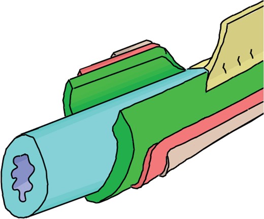
Resected cross-sectional macro-physiology of the small bowel. Moving radially outward from the center we have the inner lumenal void followed by the mucosa, submucosa (first resected layer), muscularis externa and serosa. The small bowel is anchored to the abdominal wall via the mesentery attachment (top right).

Each intestinal layer is physiologically distinct Granger & Barrowman (1984); these layers form a tube-like structure enveloping a central lumen, or inner void space, through which content passes (shaded purple in Fig. 1). Moving radially outward from the lumen is the mucosal layer (shaded blue), submucosa (shaded green), muscularis externa (shaded pink), and finally the serosa (shaded tan). The mesentery (shaded in gold) attaches the small intestine to the abdominal wall, and supplies nerve fibers, blood, and lymphatic vessels. These structures are juxtaposed, in a cut-away format, together in Fig. 1. The mucosa accounts for sixty to eighty percent of the intestinal wall thickness, and is primarily responsible for the absorption of nutrients. The submucosa makes up ten to fifteen percent of the radial thickness, and is made up of elastic fibrils, and connective tissue. The muscularis externa and serosa form a ‘muscle layer’ which lubricates and protects the intestinal tissue. The muscle layer also produces peristaltic contractions; such contractions assist in the procession of lumenal content (Granger & Barrowman, 1984; Gregersen, 2003; Johnson, 1981). We consider the muscularis externa and serosa as a combined ‘muscle layer’ due to their thinness and similar mechanical properties. Each layer of the intestine is permeated by blood capillaries and lymphatic vessels; however, vessel density is higher in the mucosal, and submucosal layers (Guyton & Hall, 2006; Miller et al., 2010). Though the capillaries and lymphatic vessels are not depicted in Fig. 1, accounting for their role in the model is the topic of Section 3.1.2. Further micro-structures, such as the epithelium lining the lumen, the villi and the microvillus protruding into the lumen from the mucosal wall, the thin muscularis mucosae bordering the mucosal and submucosal layers, etc. are not considered in the present work; details regarding these structures can be found in medical texts (Granger & Barrowman, 1984; Gregersen, 2003; Guyton & Hall, 2006).

3.1.2 Fluid balance in the interstitium

The interstitium, or intercellular region, contains an interstitial fluid phase and the structural molecules of the extracellular matrix (Wiig & Swartz, 2012). Capillaries move fluid into the interstitium, while both capillaries and lymphatics participate in the outflow of fluid from the interstitium (Sanders et al., 2014); the exchange is regulated by hydrostatic and oncotic pressure gradients. Mathematical models aimed at explaining the fluid balance in the interstitium relate microvascular filtration, mostly responsible for fluid inflow, and lymphatic return, which largely regulates fluid outflow; the difference reflects interstitial fluid storage.

$$\begin{align}& J_V(\,p) = K_F \left( P_V - p - \sigma(\varPi_V - \varPi_{I}) \right)\end{align}$$

(3.1)

$$\begin{align} J_L(\,p) = R_L^{-1}(\, p + P_p - P_L) \end{align}$$

(3.2)

Fluid balance has been studied for use in various organs such as lungs (Waaler & Aarseth, 1976; Wiener et al., 1983) and brain (Rapoport, 1978; Nagashima et al., 1990; Tully & Ventikos, 2011). The most popular model of microvascular filtration is the Starling–Landis (Landis, 1927; Pappenheimer & Soto-Rivera, 1948; Nagashima et al., 1990) equation, |$J_V$|⁠, and the Drake–Laine equation, |$J_L$|⁠, models lymph flow (Dongaonkar et al., 2008). The SLDL approach has been used for generalized interstitial spaces (Dongaonkar et al., 2008, 2009). The SLDL model employs (3.1) and (3.2) to model the balance of interstitial fluid volume, |$V$|⁠, as |$\frac{\partial }{\partial t} V = J_V(\,p) - J_L(\,p)$|⁠. This produces a linear function of the interstitial pressure, |$p$|⁠. The terms of (3.1) and (3.2) are described in Table 1. Common fluid balance modeling in the medical literature is done by solving the ODE |$\frac{\partial V}{\partial t} = J_V - J_L$| as part of a compartmental system approach; the focus is typically that of a ‘black box’ with parameter-fitting and neglects the mechanical response of the tissue (Dongaonkar et al., 2009, 2011, 2008; Taylor et al., 1990). Incorporating this response is a primary goal of the present work.

$$\begin{equation} \varPhi(\mathbf{x},p(\mathbf{x},t)) = \frac{\eta}{V_0}C(\mathbf{x}) \left( J_V(\,p(\mathbf{x},t)) - J_L(\,p(\mathbf{x},t)) \right) \end{equation}$$

(3.3)

Table 1

Terms of the Starling–Landis and Drake–Laine equations

Parameter	Description
|$K_F$|	Microvascular filtration coefficient
|$P_V$|	Microvascular hydrostatic pressure
|$\sigma $|	Protein permeability of blood capillaries (⁠|$\sigma \in [0,1]$|⁠)
|$\varPi _V$|	Microvascular oncotic pressure
|$\varPi _I$|	Interstitial oncotic pressure
|$R_L$|	Effective lymphatic resistance
|$P_P$|	Lymph pumping pressure
|$P_L$|	Hydrostatic pressure of lymph capillaries

In this work the fluid model is given by (3.3) with |$J_V$|⁠, and |$J_L$| given by (3.1)–(3.2). The additional quantities in (3.3) are as follows: |$V_0$| is a fixed reference volume that facilitates the compatibility of units with the equations of poroelasticity described in Section 3.2; |$C(\mathbf{x}) \in (0,1]$| is a dimensionless, spatial capillary distribution function where |$\mathbf{x}$| is a point in the intestinal domain; and |$\eta> 0$| is a dimensionless scaling factor. The term |$\frac{\eta }{V_0}C(\mathbf{x})$| can be interpreted as a fitted capillary density for the fluid model. An adaptation to (3.3) for the term (3.1) in the presence of high microvascular pressure and local oncontic pressure differences will be discussed in Section 4.2.

3.2 The quasi-static Biot equations of linear poroelasticity

Modeling biological tissues via the quasi-static Biot equation (Bai et al., 1993; Bear & Bachmat, 1990; Showalter, 2000) is an increasingly popular choice in biomechanics; recent models have also incorporated more than one tissue-fluid network (Tully & Ventikos, 2009; Vardakis et al., 2016, 2013). The organ is assumed as a linearly poroelastic medium consisting of an isotropic (tissue) solid skeleton permeated by a single-phase fluid. Deformations are assumed small, and inertial forces are neglected. An overview of the derivation of Biot’s equations, and generalizations to multiple fluid networks, can be found in e.g. Bai et al. (1993), Bear & Bachmat (1990) and Showalter (2000). The displacement formulation of the linear, quasi-static Biot equations for an isotropic poroelastic medium, used in this work, is given by

$$\begin{align} \frac{\partial}{\partial t} \big( c_1 p + c_0 \nabla \cdot{\textbf{w}}\big) -\kappa \varDelta p = \varPhi(\,p) \qquad\qquad\mbox{in}\quad\varOmega\times [0,T], \end{align}$$

(3.4)

$$\begin{align}-\mu\varDelta{\textbf{w}} + c_0 \nabla p -(\mu+\lambda)\nabla (\nabla \cdot{\textbf{w}}) = 0\phantom{(\,p)} \qquad\qquad\,\,\mbox{in}\quad\varOmega\times [0,T]. \end{align}$$

(3.5)

In (3.4) and (3.5) |$\mathbf{w}$| denotes the displacement of the solid (tissue) skeleton and |$p$| is the hydraulic (interstitial) pore pressure; |$\varPhi (\,p)$| is a (pressure-dependent) source function. Conservation of mass is expressed in (3.4), and (3.5) reflects conservation of momentum. The shear modulus of the tissue is |$\mu $|⁠, and |$\lambda $| is related to the tissue’s Young’s modulus. The hydraulic conductivity is denoted with |$\kappa $| and |$c_0$| is the Biot–Willis constant and |$c_1$| is the storage coefficient. Further detail of physical significance of the material parameters can be found in Bai et al. (1993) and Merxhani (2016).

3.3 A model of edema in the intestine

This section details value selection for the physical parameters and fluid balance model (3.3), applicable for the small intestine. The parameters utilized in our model are summarized in Table 2. Parameters with citations (Table 2) were garnered from the clinical literature values via a survey conducted for our previous work (Young et al., 2012). Parameter values, in Table 2 marked with an asterisk were obtained via calibration for the specific cases listed; these include the reflection coefficient, |$\sigma $|⁠, in the case of high capillary filtration (⁠|$K_f$|⁠) and the microvascular oncotic pressure (⁠|$\varPi _V$|⁠; change from baseline due to surgical trauma). The estimation of these two values, for these specific cases, is discussed in Section 4.2.

Table 2

SLxDL fluid balance model parameters |$^*$| Parameter determined via model calibration.

Starling–Landis Model
Parameter	Selected value	Units	Description	References
|$K_f$|	121.0	ml/(mmHg|$\cdot $|h)	Low pres.	Chapple et al. (1993); Gyenge et al. (1999)
	160.0	ml/(mmHg|$\cdot $|h)	High pres.	Chapple et al. (1993); Gyenge et al. (1999)
|$P_V$|	12.0	mmHg	Normal	Cox et al. (2008); Guyton & Hall (2006)
	20.0	mmHg	EVP case	Cox et al. (2008)
|$\sigma $|	0.8	-	Normal |$K_f$|	Chapple et al. (1993); Granger & Barrowman (1984); Gyenge et al. (1999)
	0.45	-	High |$K_f$|	*
|$\varPi _{V}$|	18.5	mmHg	CTRL case	*
	20.0		Normal	Brenner et al. (1972); Reed & Aukland (1977)
|$\varPi _{I}$|	12.0	mmHg	-	Gyenge et al. (1999); Reed (1995)
Drake–Laine model
Parameter	Selected avg. value	Units	Designation	References
|$R_L^{-1}$|	43.1	ml/(mmHg|$\cdot $|h)	-	Gyenge et al. (1999)
|$P_p$|	12.0	mmHg	Low pres.	Dongaonkar et al. (2011); Guyton & Hall (2006); Unno et al. (2010)
	28.0		High pres.	Dongaonkar et al. (2011); Guyton & Hall (2006); Unno et al. (2010)
|$P_L$|	2.0	mmHg	-	Dongaonkar et al. (2011)
Reference interstitial space
|$V_0$|	8400	ml	Ref. volume	Chapple et al. (1993)
|$p_{thr}$|	2.3	mmHg	Threshold pres.	Granger & Barrowman (1984); Guyton (1995)

The abbreviations CTRL and EVP refer to clinical experiments discussed in Section 4. For the capillary distribution function, |$C(\mathbf{x})$| in (3.3), a piecewise linear model is used. This choice proved most effective in exploratory work (Young & Rivière, 2011). |$C(\mathbf{x})$| obtains a maximum value |$C(\mathbf{x}_{\textrm{muc}}) = 1$| on the interface of the mucosa–lumen boundary and decreases linearly in the mucosa to the submucosa. In the submucosa the value is |$C(\mathbf{x}_{\textrm{submuc}}) = 0.001$|⁠, and in the musculature the value is |$C(\mathbf{x}_{\textrm{musc}}) = 0.002$|⁠. This reflects the relative distribution of capillaries within the intestinal structure (Granger & Barrowman, 1984); Fig. 2 shows a graph of the distribution superimposed on a test mesh. To specify the poroelasticity model for the intestine some adaptations are necessary. The internal physiology of the intestine is layered (see Fig. 1). Each layer is characterized by its own set of |$(\mu ,\lambda )$| parameters (Cox et al., 2008). Within each layer the isotropic, quasi-static, linearly poroelastic assumptions are assumed to hold.

$$\begin{equation} \mu(\,p),\,\lambda(\,p) = \left\{ \begin{array}{@{}cc} \mu_1,\,\lambda_1 & p < p_{thr} \\ \mu_2,\,\lambda_2 & p \geqslant p_{thr} \end{array} \right. \end{equation}$$

(3.6)

Clinical experiments have shown that the values of |$\mu $| and |$\lambda $| in the intestine are pressure dependent (Granger & Barrowman, 1984; Guyton, 1995; Radhakrishnan et al., 2005), i.e. |$\mu = \mu (\,p)$| and |$\lambda = \lambda (\,p)$|⁠. This effect could be due to local connective tissue degradation at high pressure. More specifically, clinical experiments (Radhakrishnan et al., 2005; Cox et al., 2008) investigated changes to |$\mu $| and |$\lambda $| in the presence of edema by performing stretch and opening angle (Vaishnav & Vossoughi, 1987; Gregersen, 2003) measurements on tissues in various stages of induced edema. It was shown (Radhakrishnan et al., 2005) that as the venous pressure increased, i.e. increased severity of induced edema, differences in the specimen elastic properties were observed. In Cox et al. (2008) high venous pressures were correlated to elevated interstitial pressure; further establishing the suggestive relation |$\mu = \mu (\,p)$| and |$\lambda =\lambda (\,p)$|⁠. In our earlier work (Young & Rivière, 2011; Young et al., 2012) the pressure-dependent changes to |$\mu $| and |$\lambda $| were established in collaboration with the authors of the original clinical study (Cox et al., 2008) based on their laboratory measurements. It is assumed that the pressure dependence is piecewise constant and based on a threshold pressure, |$p_{thr}$| as in (3.6). Pressure-dependent values (Collinsworth et al., 2002; Cox et al., 2008; Granger & Barrowman, 1984; Guyton, 1995; Radhakrishnan et al., 2005) of |$\mu $| and |$\lambda $| are shown in Table 3. The scaling relation |$c_1 \approx \lambda ^{-1}$| has also been assumed (Lee et al., 2017; Merxhani, 2016) and is incorporated into the model via: |$p>p_{thr}$| implies |$c_1 \rightarrow c_1(\lambda _1/\lambda _2)$|⁠.

Table 3

Lamé parameters (in mmHg)

|$p < p_{thr}$|						|$p \geqslant p_{thr}$|
	Mucosa	Submucosa	Muscle		Mucosa	Submucosa	Muscle
|$\mu $| (mmHg)	3	1050	120		1.5	750	60
|$\lambda $| (mmHg)	7.5	2625	300		3.75	1875	150

For pressure exceeding |$p_{thr}$| the shift in |$(\mu ,\lambda ,c_1)$| reflects the damaged state of the respective intestinal layer. For this simplified damage model (Radhakrishnan et al., 2005; Cox et al., 2008) the values of |$\mu $| and |$\lambda $| are changed within a layer once the average pressure of that layer exceeds |$p_{thr}$|⁠. Localized damage models, based on clinical studies of soft-tissue injury under high pressures, may further refine results.

The remaining model values to be specified are the hydraulic conductivity |$\kappa $|⁠, Biot–Willis coefficient |$c_0$| and storage coefficient |$c_1$|⁠; see Table 4. The hydraulic conductivity is assumed uniform and estimated from studies conducted on whole bovine trachea (Durand et al., 1981); the physiology of the trachea is layered, and similar to the intestine. A common assumption in soil models (Bai et al., 1993), also reasonable for soft tissues (Doblare & Merodio, 2015), is that the Biot–Willis coefficient is |$c_0 \approx 1$|⁠. Following Vardakis et al. (2016) we select |$c_0 = 0.99$|⁠, and |$c_1 = 4.5\times 10^{-10}$||$Pa^{-1}$|⁠. Due to the transition of tissue composition between the mucosa and muscle layer we estimate |$c_1$| in the submucosa as one order of magnitude lower and two orders of magnitude lower in the muscle layer.

Table 4

Coefficients in Biot’s model

Biot–Willis |$(c_0)$|	Storage (⁠|$c_1$|⁠, mucosa)	Hydraulic conductivity (⁠|$\kappa $|⁠)
0.99	|$4.5\times 10^{-10}$||$Pa^{-1}$|	|$ 4.540\times 10^{-13}$||$m^2/Pa\cdot s$|

Fig. 2.

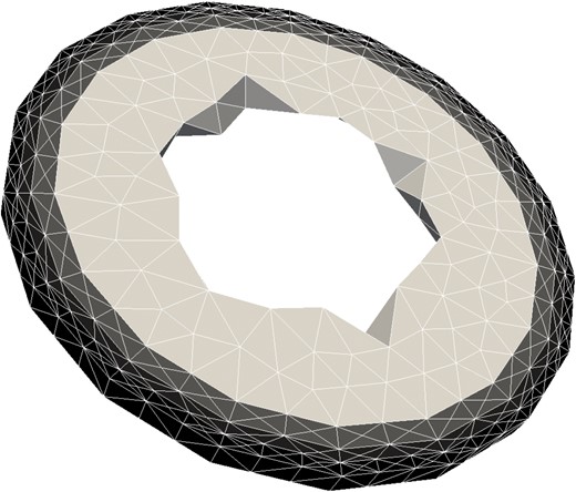
|$C(\mathbf{x})\in (0,1]$|⁠. Higher values are darker

3.4 An implicit DG discretization

In this section we discuss an extension to a previously proposed (Rivière et al., 2017) implicit in time DG discretization for a mixed formulation of (3.4) and (3.5) for use with clinical simulations of intestinal edema. Section 3.4.1 describes the mixed formulation of (3.4) and (3.5) and Section 3.4.2 details the extension of the discrete scheme presented found in Rivière et al. (2017). Early models for intestinal edema have used an explicit-in-time discretization (Young et al., 2012), which relies on the assumption that the constrained storage coefficient is zero. Not only is this assumption physiologically inaccurate in the intestine but also explicit in time discretizations can affect the stability condition of the method resulting in a restrictive time step size (Booker & Small, 1975; Miga et al., 1998; De La Puente et al., 2008). Early investigation (Booker & Small, 1975) of a Lagrange finite element discretization of Biot’s equation examined the |$\theta $| family of one-step time-discretization methods given by

$$\begin{equation*} y^{n+1} - y^n \approx \varDelta t \left( \theta f(t^n,y^n) + (1-\theta)f(t^{n+1},y^{n+1})\right). \end{equation*}$$

It was shown that the resulting time-space discretization was unconditionally stable for |$\theta \leqslant \frac 12$|⁠. For |$\theta> \frac 12$| a restrictive stability requirement was needed. A Von Neumann stability analysis (Miga et al., 1998) later showed that for fully saturated porous media explicit schemes (⁠|$\theta = 1$|⁠) are infeasible for general use and controlling spurious oscillations in the pore pressure requires a fully implicit (⁠|$\theta = 0$|⁠) time integration scheme.

3.4.1 A mixed formulation of Biot’s equations and boundary conditions

Define the dilatation |$\epsilon = \nabla \cdot \mathbf{w}$| extending equations (3.4) and (3.5) and consider the following mixed form of Biot’s equations:

$$\begin{align} -\mu\varDelta{\textbf{w}} + c_0 \nabla p -(\mu+\lambda)\nabla\varepsilon & = 0,\quad\mbox{in}\quad\varOmega\times [0,T], \end{align}$$

(3.7)

$$\begin{align} \nabla \cdot{\textbf{w}} -\varepsilon & = 0,\quad\mbox{in}\quad\varOmega\times [0,T], \end{align}$$

(3.8)

$$\begin{align} c_1 \frac{\partial p}{\partial t} + c_0\frac{\partial \varepsilon}{\partial t} -\kappa \varDelta p & = \varPhi(\,p),\quad\mbox{in}\quad\varOmega\times [0,T]. \end{align}$$

(3.9)

|$\varOmega \subset \mathbb{R}^{d}$| is assumed to be a bounded, convex domain, with smooth boundary |$\partial \varOmega $|⁠. The boundary is decomposed into disjoint Dirichlet and Neumann sections, for the displacement and pressure, by |$\partial \varOmega = \varGamma _{wD}\cup \varGamma _{wN}$| and |$\partial \varOmega = \varGamma _{pD}\cup \varGamma _{pN}$| where |$\varGamma _{wD}\cap \varGamma _{wN} = \varGamma _{pD}\cap \varGamma _{pN} = \emptyset $|⁠.

$$\begin{equation} \begin{array}{cc} p = p_D & \textrm{ on}\ \varGamma_{pD}\times(0,T) \\ \kappa \nabla p\cdot\mathbf{n} = g_p & \textrm{ on}\ \varGamma_{pN}\times(0,T)\\ & \\ \mathbf{w} = \mathbf{w}_D & \textrm{ on}\ \varGamma_{wD} \times(0,T)\\ \mu\nabla\mathbf{w}\cdot\mathbf{n} + (\mu+\lambda)\varepsilon\mathbf{n} - c_0 p \mathbf{n} = g_{W} & \textrm{ on}\ \varGamma_{wN}\times(0,T) \end{array} \end{equation}$$

(3.10)

The boundary conditions considered for the model are presented in (3.10). Pressure is prescribed on |$\varGamma _{pD}$|⁠, and displacement is prescribed on |$\varGamma _{wD}$|⁠, while on |$\varGamma _{pN}$| a Darcy flux is imposed. On |$\varGamma _{wN}$| the displacement formulation of the Cauchy normal stress condition, |$\sigma \cdot \mathbf{n} = g_W$| where |$\sigma $| is the Cauchy stress tensor, is enforced. In our application, |$g_W = 0$| is used on |$\varGamma _{wN}$|⁠, |$g_p = 0$| on |$\varGamma _{pN}$| and the boundary measure of the set |$\varGamma _{pD}$| is zero. More details on the boundary locations for the intestinal geometry will be discussed in Section 4.3.

3.4.2 Discretization and an extension to the intestinal model

The (intestinal) domain |$\varOmega $| is triangulated with a quasi-uniform (Rivière, 2005) tetrahedral mesh |${\boldsymbol T}_h$| with maximum element diameter denoted |$h$|⁠. Equations (3.7)–(3.9) are then discretized in space via the DG method (Rivière, 2005). The discretization follows the procedure in Rivière et al. (2017), with a slight extension; the purpose of this section is to briefly describe the extension to the bilinear forms appearing in the previous work and refer the interested reader there for more details.

The discretization of the mixed equations 3.73.9 is carried out in Rivière et al. (2017) under the assumption of constant lame parameters |$\mu $| and |$\lambda $|⁠. As discussed in Section 3.3 clinical experiments show that |$\mu $| and |$\lambda $| take on different values in each layer of the intestine and are pressure dependent (Granger & Barrowman, 1984; Guyton, 1995; Radhakrishnan et al., 2005). In the present work it is assumed that the Lamé parameters satisfy a piecewise constant dependence on the pressure; see e.g. Table 3, (3.6) and the value of |$p_{thr}$| in Table 2. Toward this let |$\tilde{\mu }(\,p)$| and |$\tilde{\lambda }(\,p)$| denote element-wise constant approximations to the pressure-dependent parameters |$\mu (\,p)$| and |$\lambda (\,p)$|⁠. In this manuscript |$\tilde{\mu }(\,p)$| and |$\tilde{\lambda }(\,p)$| are defined by evaluating the numerical pressure at the barycenter of each element and using (3.6). Let |$M_h\times M_h\times{\textbf{V}}_h$| be the discrete DG spaces defined as in Rivière et al. (2017). Then the extended discrete scheme [compare to e.g. equations (10)–(11) in Rivière et al., 2017] can be stated as follows:

Given |$(\,p_h^n,\varepsilon _h^n,{\textbf{w}}_h^n)$| in |$M_h\times M_h\times{\textbf{V}}_h$|⁠, find |$(\,p_h^{n+1},\varepsilon _h^{n+1},{\textbf{w}}_h^{n+1})$| in |$M_h\times M_h\times{\textbf{V}}_h$| such that for every |$(r,q,{\textbf{v}})\in (M_h\times M_h\times{\textbf{V}}_h)$| we have

$$\begin{align} &c_1 \left(\frac{p_h^{n+1}-p_h^n}{\varDelta t}, r\right)_\varOmega +c_0\left(\frac{\varepsilon_h^{n+1}-\varepsilon_h^n}{\varDelta t}, r\right)_\varOmega + \kappa a_1\left(\,p_h^{n+1},r\right) \nonumber \\ & \quad= \left(\varPhi\left(\,p_h^{n}\right),r\right)_\varOmega + \ell_1(t^{n+1};r), \quad \forall n\geqslant 0, \end{align}$$

(3.11)

$$\begin{align} &\left(\varepsilon_h^{n+1},q\right)_\varOmega+b\left({\textbf{w}}_h^{n+1},q\right) = \ell_2(t^{n+1};q),\quad \forall n \geqslant -1, \end{align}$$

(3.12)

$$\begin{align} & a_{2,\mu}\left({\textbf{w}}_h^{n+1},{\textbf{v}}\right)+j\left(\frac{{\textbf{w}}_h^{n+1}-{\textbf{w}}_h^n}{\varDelta t},{\textbf{v}}\right) - b_{\mu+\lambda}\left({\textbf{v}},\varepsilon_h^{n+1}\right) + c_0 b\left({\textbf{v}},p_h^{n+1}\right) \nonumber \\ &\qquad \quad= \ell_3(t^{n+1};{\textbf{v}}) + \sum_{e\in\varGamma_{\mathrm{wD}}} \frac{\sigma_2}{h_e} \left(\frac{{\textbf{w}}_D(t^{n+1})-{\textbf{w}}_D(t^n)}{\varDelta t},\right)_e,\quad \forall n\geqslant 0. \end{align}$$

(3.13)

The only modifications in (3.11)–(3.13) to those of the previous work [equations (10)–(11) in Rivière et al., 2017] are those made to the bilinear forms of (3.12) and (3.13). These have been altered by

$$\begin{align} a_{2,\mu}({\textbf{w}},{\textbf{v}}) &= \sum_{E\in{\boldsymbol T}_h} (\tilde{\mu}(\,p)\nabla{\textbf{w}},\nabla{\textbf{v}})_E - \sum_{e\in\varGamma_h\cup\varGamma_{\mathrm{wD}}}(\{ \tilde{\mu}(\,p) \nabla{\textbf{w}}\}\cdot{\textbf{n}}_e,[{\textbf{v}}])_e \nonumber \\ & \quad+ \theta_2 \sum_{e\in\varGamma_h\cup\varGamma_{\mathrm{wD}}}(\{\tilde{\mu}(\,p)\nabla{\textbf{v}}\}\cdot{\textbf{n}}_e,[{\textbf{w}}])_e + \sum_{e\in\varGamma_h\cup\varGamma_{\mathrm{wD}}}\frac{\sigma_2}{h_e}\left\{\tilde{\mu}(\,p)\right\}([{\textbf{w}}],[{\textbf{v}}])_e, \end{align}$$

(3.14)

$$\begin{eqnarray} b_{\mu+\lambda}({\textbf{v}},q) = -\sum_{E\in{\boldsymbol T}_h} (\nabla\cdot{\textbf{v}},q)_E + \sum_{e\in\varGamma_h\cup\varGamma_{\mathrm{wD}}}\left(\left\{\big( \tilde{\mu}(\,p)+\tilde{\lambda}(\,p) \big) q\right\},[{\textbf{v}}]\cdot{\textbf{n}}_e\right)_e\!. \end{eqnarray}$$

(3.15)

More specifically, in Rivière et al. (2017) the Lamé parameters |$\mu $| and |$\lambda $| were assumed constant throughout the medium. In accordance with the damage model discussed in Section 3.3 the pressure-dependent Lamé parameters still assume constant values within a layer. Thus, within the same layer, (3.14) and (3.15) simplify to those previously analyzed (Rivière et al., 2017) and are given by

$$\begin{align*} a_{2,\mu}({\textbf{w}},{\textbf{v}}) &= \sum_{E\in{\boldsymbol T}_h} \tilde{\mu}(\nabla{\textbf{w}},\nabla{\textbf{v}})_E - \sum_{e\in\varGamma_h\cup\varGamma_{\mathrm{wD}}} \tilde{\mu}(\nabla{\textbf{w}}\cdot{\textbf{n}}_e,[{\textbf{v}}])_e \nonumber \\ & \quad+ \theta_2 \sum_{e\in\varGamma_h\cup\varGamma_{\mathrm{wD}}} \tilde{\mu}(\nabla{\textbf{v}}\cdot{\textbf{n}}_e,[{\textbf{w}}])_e + \sum_{e\in\varGamma_h\cup\varGamma_{\mathrm{wD}}}\frac{\sigma_2}{h_e}\tilde{\mu}([{\textbf{w}}],[{\textbf{v}}])_e, \end{align*}$$

$$\begin{eqnarray*} b_{\mu+\lambda}({\textbf{v}},q) = -\sum_{E\in{\boldsymbol T}_h} (\nabla\cdot{\textbf{v}},q)_E + \sum_{e\in\varGamma_h\cup\varGamma_{\mathrm{wD}}}(\tilde{\mu}+\tilde{\lambda})(\{q\},[{\textbf{v}}]\cdot{\textbf{n}}_e)_e. \end{eqnarray*}$$

The scheme used in the biomedical computations for the intestine is therefore given by (3.11)–(3.15) where |$\varPhi (\,p^n)$|⁠, in (3.11), is defined by (3.3). In practice, we take |$\theta _1 = \theta _2 = 1$| (appearing in the bilinear forms |$a_1(\,p_h,q_h)$| and |$a_{2,\mu }({\textbf{w}}_h,{\textbf{v}}_h)$|⁠) as the non-symmetric (NIPG) variant of the scheme that was shown to be more robust to non-physical pressure oscillations often seen in discretizations of Biot’s equations (Rivière et al., 2017). The penalty value used for |$\sigma _2$|⁠, in (3.14), is |$1\times 10^1$| while the penalty value used for |$\sigma _1$|⁠, analogously defined in the bilinear form |$a_1(\,p_h,r)$| of (3.11), is |$1\times 10^{-2}$|⁠.

3.4.3 Summary of numerical method a priori behavior

The simulations described in Section 4 utilize the numerical method given by (3.11)–(3.15); to facilitate computational cost considerations the discrete spaces, |$M_h$| (pressure and dilatation) and |$V_h$| (displacement) were chosen to consist of element-wise linear DG functions. When the Lamé parameters agree on both elements of a common edge, such as within the same intestinal layer, (3.14)–(3.15) reduce to a discrete scheme for constant Lamé parameters studied by the authors in a previous work (Rivière et al., 2017). In Rivière et al. (2017) we endeavored an extensive a priori convergence analysis for both NIPG and SIPG variants of the approach. In this section we briefly recall our a priori convergence result for the NIPG discretization and refer the interested reader to Rivière et al. (2017) for a full discussion and formal proof. Assume that the Lamé coefficients are constant throughout the domain, as is the case within each intestinal layer, then in Rivière et al. (2017) we have proven the following result for the NIPG method:

 

Theorem 3.1

(The NIPG method).

Assume that |$\varDelta t < 1$|⁠, |$c_1>0$| and that |$\theta _2 = 1$| in (3.14) so that the form |$a_{2,\mu }$| is non-symmetric. Let |$k_m$| denote the polynomial degree of the DG space |$M_h$|⁠, |$k_v$| the polynomial degree of the DG space |$V_h$| and |$L_{\varPhi }$| the Lipschitz continuity constant of the source function |$\varPhi $|⁠. Then there exists a constant |$C$| independent of |$h$|⁠, |$\varDelta t$|⁠, as well as |$c_0, \kappa , \lambda $| such that for any |$m\geqslant 1$|⁠:

$$\begin{equation*} c_1 \big|\big| p^{m}-p_h^m\big|\big|_{L^2(\varOmega)}^2 \leq C h^{2k_m} c_1 || p^m||_{H^{k_m+1}(\varOmega)}^2+\mathcal{B}, \end{equation*}$$

$$\begin{equation*} (\mu+\lambda) \big|\big| \epsilon^{m}-\epsilon_h^m\big|\big|_{L^2(\varOmega)}^2 \leq C (\mu+\lambda) h^{2k_m} || \epsilon^m||_{H^{k_m+1}(\varOmega)}^2 +\mathcal{B}, \end{equation*}$$

$$\begin{equation*} \varDelta t \kappa \sum_{n=1}^{m} \big|\big| p^{n}-p_h^{n}\big|\big|_M^2 \leq \kappa C h^{2k_m} || p||_{L^\infty(0,T;H^{k_m+1}(\varOmega))}^2 +\mathcal{B}, \end{equation*}$$

$$\begin{equation*}\mu \big|\big|{\textbf{w}}^{m}-{\textbf{w}}_h^m\big|\big|_{\textbf{V}}^2 \leq \mu C h^{2k_v} || {\textbf{w}}^m ||_{H^{k_v+1}(\varOmega)}^2 +\mathcal{B},\end{equation*}$$

where the quantity |$\mathcal{B}$| is defined as

$$\begin{eqnarray*} & \mathcal{B} = C(\mu,c_1,T) \left(\mathcal{A} + C \mu h^{2k_v} || {\textbf{w}}||_{L^\infty(0,T;H^{k_v+1}(\varOmega))}^2\right), \end{eqnarray*}$$

and |$\mathcal{A}$| is defined by

$$\begin{eqnarray*} & \mathcal{A} = C(c_1,T) \left( \left(\frac{L_\varPhi^2}{\kappa}+c_0^2+\kappa\right) h^{2 k_m} || p||_{L^\infty(0,T;H^{k_m+1}(\varOmega))}^2\right. \nonumber \\ & +\, h^{2 k_m+2} (\mu+\lambda)^2 || \epsilon||_{L^\infty(0,T;H^{k_m+1}(\varOmega))}^2 + \left(1+\frac{c_0^2}{\kappa}+ (\mu+\lambda)\right)h^{2 k_v} || {\textbf{w}}_t||_{L^\infty(0,T;H^{k_v+1}(\varOmega))}^2 \nonumber \\ & + \,(\mu+\lambda) C h^{2k_v} || {\textbf{w}}_0||_{H^{k_v+1}(\varOmega)}^2 + \frac{\varDelta t^2}{\kappa} \left(c_1^2 \right.|| p_{tt}||_{L^\infty(0,T;L^2(\varOmega))}^2\nonumber \\ & \left. + \,c_0^2 || \epsilon_{tt}||_{L^\infty(0,T;L^2(\varOmega))}^2 + L_\varPhi^2 || p_t ||_{L^\infty(0,T;L^2(\varOmega)}^2\big)\phantom{\frac{L_\varPhi^2}{\kappa}}\right). \end{eqnarray*}$$

In particular, the a priori analysis predicts optimal convergence rates for the dilatation, pressure and displacement in the |$L^2$|⁠, |$M$| and |$V$| norms, respectively; here, the |$M$| and |$V$| norm notation represents the standard DG energy norm (Rivière, 2005) on the corresponding spaces. Optimal |$L^2$| convergence rates for the pressure and displacement errors were observed computationally (Rivière et al., 2017). Moreover, an implication of the above is that the best overall convergence rates are achieved when |$k_m = k_v$|⁠; i.e. when the DG spaces |$M_h$| and |$V_h$| are chosen to be of the same polynomial degree. We close this section by re-iterating that several additional results, such as the symmetric (SIPG) scheme and when the storage coefficient, |$c_1$|⁠, vanishes, are discussed in our previous work (Rivière et al., 2017). In addition, the interested reader will find that a numerical study of spurious pressure oscillations has been conducted and that the predicted convergence rates have been verified, in both time and space, using the method of manufactured solutions.

4. Numerical simulations of a clinical experiment

The suitability of the computational model for clinical applications is tested via comparison to a published medical experiment (Cox et al., 2008) from the Center for Microvascular and Lymphatic Studies, at the University of Texas-Houston Medical School, in conjunction with the DeBakey Institute at Texas A&M University. Section 4.1 is an overview of the clinical experiment while Section 4.2 relates the experiment and the mathematical model; Section 4.3 covers details of the numerical implementation; Section 4.4 discusses results of the direct computational analogs carried out in the clinical experiment. Section 4.1 overviews the clinical study (Cox et al., 2008) of interest and Section 4.2 discusses the link between the constituent clinical experiments and the mathematical model.

4.1 Experimental procedure

The overall focus of a recent clinical study (Cox et al., 2008) was to investigate whether acute edema may impair the contractile function of the intestine and to judge the effects of |$7.5\%$| HS resuscitation in abetting acute edema expression. The effects of intestinal edema were investigated via four clinical experiments on male Sprague-Dawley rats: a control case (CTRL), a |$7.5\%$| HS infusion, an EVP case, and an EVP followed by |$7.5\%$| HS administration (EVP-HS). Each group was anesthetized 12–16 hours before surgical procedure, and fasted. A silastic catheter was placed into the main intestinal lymphatic vessel, the superior mesenteric vein was dissected free of its mesenteric attachment and a pressure transducer catheter was inserted into the submucosal layer of the small intestine.

The four treatments are as follows: the CTRL group received a sham (placebo) surgical procedure. The EVP group was given a large infusion of normal saline and a suture of the mesenteric vein to induce EVP. The HS group received a small infusion HS. The EVP-HS group was given a large infusion of normal saline, suturing of the mesenteric vein and halfway through the experiment a small infusion HS. Submucosal pressure measurements were taken at 30 minutes after preparation. In addition to the submucosal pressure measurements, the interstitial fluid volume gain was also estimated for the EVP case via a wet–dry ratio measurement process. Table 5 provides a quick reference to the experimental abbreviations and descriptions.

Table 5

Clinical experiments of Cox et al. (2008)

Abbrev.	Description
CTRL	Sham surgical procedure
EVP	Large infusion of normal saline, and a suture to
	induce EVP
HS	An infusion of HS
EVP-HS	A large infusion of normal saline, a suture to induce
	EVP, an infusion of HS midway

4.2 Experimental relationship to the mathematical model

Modeling the clinical experiment relies primarily on the modulation of four parameter values from (3.3): |$K_f$|⁠, |$P_V$|⁠, |$\varPi _V$| and |$P_p$|⁠. Normal clinical ranges for these values are shown in Table 6. The CTRL case was used to calibrate a baseline oncotic blood pressure |$\varPi _V$|⁠. Following a surgical procedure |$\varPi _V$| can be slightly lower than normal in vivo values due to incurred trauma (Böck et al., 1989; Golab et al., 2011; Lucas et al., 1982; Öhqvist et al., 1980). Likewise, capillary physiology can change substantially in the presence of EVP exceeding |$15$| mmHg (Scallen et al., 2010); the EVP case was therefore used to calibrate the |$K_f-\sigma $| change relationship; more details are given below. Variation of the parameters in the clinical experiment were as follows: in the CTRL and HS case a value of |$12$| mmHg was used for |$P_V$|⁠. In the EVP and EVP-HS cases the suturing procedure produced |$P_V$| measured in the ranges of |$17$|–|$23$| mmHg; the median value of |$20$| mmHg was used in the EVP and EVP-HS computations. For the CTRL and HS cases, a baseline value of |$P_p = 15$| mmHg was used. The lymphatic system is known to respond to higher venous pressure with increased lymph flow (Guyton & Hall, 2006), and so in the case of EVP and EVP-HS, a value of |$28$| mmHg was used for |$P_p$|⁠.

Table 6

Normal clinical parameter ranges

Clinical ranges of experimental parameters
Parameter	Range	References
|$P_V$|	10.0–12.0 mmHg	Cox et al. (2008); Guyton & Hall (2006)
|$\varPi _{V}$|	20.0–25.9 mmHg	Gyenge et al. (1999); Reed (1995)
|$K_f$|	121–200 (ml/mmHg|$\cdot $|h)	Chapple et al. (1993); Gyenge et al. (1999)
|$P_p$|	10.0–30.0 mmHg	Dongaonkar et al. (2011); Guyton & Hall (2006);
		Unno et al. (2010)

For the cases CTRL and HS the normal baseline value for |$K_f$| of |$121$| ml/mmHg was used. In the case of EVP and EVP-HS the suture-induced high values of |$P_V$| cause a stretching of the endothelial layer of the vessels; this raises the value of |$K_f$| and lowers the value of |$\sigma $|⁠, the reflection coefficient in (3.3), commensurately Scallen et al. (2010); this dynamic has been observed experimentally (Maron et al., 2001). A value of |$K_f = 160$| mmHg was used in the EVP and EVP-HS cases, the EVP case was then used to find a compatible value of |$\sigma $|⁠. Computations were matched to the clinically reported average submucosal pressure for the EVP case yielding a value of |$\sigma =0.45$|⁠; this value is also used for the EVP-HS case before the administration of HS. The baseline normal (Gamble et al., 1988) physiological value of |$\sigma =0.8$| was used in both the CTRL and HS cases as |$K_f$| was taken in the normal physiological range.

The oncotic blood pressure, |$\varPi _V$|⁠, is altered primarily in two ways relevant to the experimental tests. First, a drop in oncotic blood pressure due to surgical preparation procedures can occur for various reasons, including blood loss or the trauma of the surgery itself (Böck et al., 1989; Golab et al., 2011; Lucas et al., 1982; Öhqvist et al., 1980). The CTRL case computations were matched to clinical experimental average results by altering only |$\varPi _V$| to gauge surgical impact to baseline oncotic pressure. This resulted in a slight decrease in |$\varPi _V$|⁠, below normal homeostatic conditions, to |$18.5$| mmHg. This value was used in the CTRL and EVP experiments. Secondly, when vascular oncotic pressure, |$\varPi _V$|⁠, is low administration of HS is known to expand local plasma volume, increasing |$\varPi _V$| to near-normal levels (Fisher et al., 1992; Kinsky et al., 2000; Mazzoni et al., 1988), though this resuscitation effect can wane after several hours due to blood-protein washdown effects. The experimental time window, at 30 minutes, is not long enough to warrant inclusion of protein-washdown effects in the model; thus, we take |$\varPi _V = 20$| mmHg, the normal value, in the cases of HS and EVP-HS post-injection of HS. Finally, an increase in |$\varPi _V$| coincides with a decreases in |$K_f$| (Guyton & Hall, 2006); thus, in the EVP-HS post-injection case |$K_f$| is returned to the baseline value of |$K_f = 121$| ml/mmHg and |$\sigma $| is returned to the normal value of |$\sigma =0.8$| to reflect the resuscitation effect of HS.

$$\begin{equation} \varPhi(\mathbf{x},p(\mathbf{x},t)) = \frac{\eta}{V_0}C(\mathbf{x}) \left( \mathcal{J}_V(\,p(\mathbf{x},t)) - J_L(\,p(\mathbf{x},t)) \right) \end{equation}$$

(4.1)

The parameter quantities discussed for use in the experimental simulation are given summarized in Table 7. The EVP-HS experiment is characterized by values separated by a slash to demarcate the pre-injection (left) values from the post-injection (right) values for the HS administered at the halfway mark of the procedure. We close this section with a mention of a correctional modification to the fluid balance (3.3) for the EVP-HS case. Recent experiments (Hu et al., 2000; Levick, 2004) have observed that the Starling equation overestimates the vascular filtration rate in the case of high |$P_V$|⁠, exceeding |$15$| mmHg, and the introduction of local oncotic pressure gradients such as via albumin perfusates. HS injection expands local plasma volume, raising |$\varPi _V$| locally on one side of the endothelium, and the model takes this into account by using a corrected Starling equation that takes the form |$\mathcal{J}_V = (1/M) J_V$|⁠; see (3.3) versus (4.1). A correction factor can be estimated from experimental clinical data (Hu et al., 2000) on Starling overestimation in this context. The correction factor |$M=2.75$| is used in the model for the EVP-HS case post HS injection; for all other cases, including EVP-HS pre-injection of HS, |$M=1$| and |$\mathcal{J}_V = J_V$| as expected.

Table 7

Representative rxperimental model parameters

Numerical values for clinical experiments
Experiment	|$P_V$|	|$\varPi _V$|	|$K_f$|	|$P_p$|	|$\sigma $|
CTRL	12	18.5	121	15	0.8
HS	12	20	121	15	0.8
EVP	20	18.5	160	28	0.45
EVP-HS	20	18.5 / 20	160 / 121	28	0.45 / 0.8

4.3 Implementation of the numerical scheme

The NIPG variant of (3.11)–(3.13) is used to carry out the computations; in a previous work (Rivière et al., 2017) this approach was more robust in alleviating possible spurious oscillations in the numerical pressure when used with differing values of |$\sigma _1$| and |$\sigma _2$|⁠. As discussed, |$\sigma _1 = 1\times 10^{-2}$|⁠, and |$\sigma _2 = 1\times 10^{1}$| for the simulations in this manuscript. The scheme (3.11)–(3.15) was implemented using the C programming language, using PETSc (Balay et al., 2017a,b, 1997) to assemble and solve the linear system. Preconditioning schemes for Biot-type problems are an ongoing field of research (Lee et al., 2017); to avoid any issues with experimental comparison, from e.g. preconditioning or iterative solver choice, SuperLU (Li et al., 2011; Li, 2005; Li & Shao, 2011) was used to facilitate a direct solve via LU factorization. The small bowel of a Sprague-Dawley rat has an approximate radius of |$r=0.18$| cm (Griffin & O’Driscoll, 2008); to-scale meshes were created using Gmsh (Geuzaine & Remacle, 2009). Fig. 3 shows a view of a single slice of the basic geometry, the mucosa being the lightest inner layer, then the submucosa (gray) and the combined musculature (black) layers of the muscularis externa and the serosa. The first 3D section is defined in the |$x$|–|$y$| plane, and further layers are then stacked in the +Z direction. The Lamé parameters being a constant value within each layer of the intestine is enforced in the model through the use of the average pressure. After each time step the layer average pressure is computed from the previous pressure solution; if the layer’s average pressure exceeds the threshold value |$p_{thr}$|⁠, see Table 2, the layer’s Lamé parameters are modified via (3.6) and Table 3. The change in tissue Lamé parameters is speculated to be caused by a breakdown in connective tissues due to the high pressure load. Once a tissue layer has been damaged it remains in the damaged state for the duration of the simulation.

Fig. 3.

Thin slice of a rat small intestine

Fig. 4.

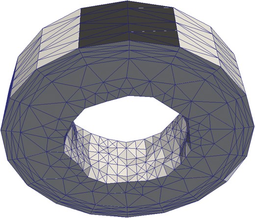
Mesentery boundary faces

Let |$\varGamma =\partial \varOmega $| denote the boundary of the computational domain, |$\varOmega $|⁠. For the pressure we take the Neumann boundary to be |$\varGamma _{pN} = \varGamma $| and |$g_p = 0$|⁠. From a physical perspective this means that the interstitial fluid cannot penetrate the boundary. For the displacement a homogeneous Dirichlet boundary condition, |$\mathbf{w} = 0$|⁠, is symmetrically imposed on the top of the intestinal mesh for the faces constituting |$\approx 10\%$| of the radial surface area; physiologically, this reflects the anchoring of the intestine by the mesentery; see Fig. 4 where mesentery boundary faces are indicated in black. The condition |$\mathbf{w}=0$| is also imposed on the outermost faces, those with outward normal in the +Z or -Z axis direction. On all remaining faces the zero stress condition, of (3.10), is imposed; condition (3.10) is equivalent to |$\sigma \cdot \mathbf{n} = 0$| where |$\sigma $| is the usual total stress tensor (Showalter, 2000) of Biot’s equations; physiologically, this implies that these faces are free to deform.

Table 8

Average computed submucosal pressures (Pa). Model calibration cases are shown in bold.

Average submucosal pressures
Experiment	6 min	12 min	18 min	24 min	30 min
CTRL	34.3	63.1	86.2	104.8	119.5
EVP	241.3	231.3	335.3	426.4	505.7
HS	13.4	24.6	33.7	41.0	46.7
EVP-HS	241.3	231.3	265.2	206.2	149.5

 

Remark 4.1

The Dirichlet condition |$\mathbf{w}=0$| imposed on the end-cap face, those with outward facing normal in the +Z or -Z direction, reduces the capacity for tetrahedra in the outer layers to deform. It was found that using at a mesh consisting of at least five layers provides an acceptable balance, in practice, between computational complexity and capacity for layer deformation to closely approximate clinical results.

For the numerical tests, linear DG approximations were used for the displacement, dilatation and pressure approximations. Meshes consisting of five layers balanced computational efficiency, with clinical results. All clinical quantities reported in Tables 2, 4 and 6 were converted to standard units of Pascals for pressure, milliliters for volume, seconds for time and meters for length; all meshes were constructed at the physical scale of an intestine for a fully matured male Sprague-Dawley rat.

4.4 Primary computational results

In this section the primary results of the computational experiments, e.g. those that can be most directly assessed against a corresponding clinical experiment (Cox et al., 2008), are discussed. Each of the computational experiments will be covered, beginning with the primary calibration cases; these are the CTRL and EVP cases. As mentioned in Section 4.1 the primary clinical point of comparison (Cox et al., 2008) are the submucosal pressure measurements derived, therein, from a pressure transducer reading. For comparison with this reading an average pressure within an intestinal layer, |$\varOmega _L$|⁠, was computed using the canonical average value

$$\begin{equation} p_{\textrm{ave},L} = \frac{1}{|\varOmega_{L}|} \int_{\varOmega_L} p \, \textrm{dx}. \end{equation}$$

(4.2)

The domain |$\varOmega _L$| could be the mucosa, submucosa or musculature; although only measurements for the submucosa were available for comparison with experiment. For each computational experiment this section details any pertinent calibrated values, final average submucosal pressure, overall minimum–maximum pressure ranges and local-in-time minimum–maximum pressure ranges. A summary of the relevant pressure values for the section can be found in Tables 8 and 9. One distinct advantage of developing, and utilizing, computational models of intestinal edema is the ability to explore additional features of the clinical experiment in a manner unencumbered by practical clinical problems such as e.g. difficulties in transducer placement within a particular intestinal layer. Toward this end, further analysis of the computational results, including observations, predictions and suggested clinical experiments, will be covered in Section 5.

Table 9

Computed pressure ranges by experiment. Min pressure–max pressure (Pa). |$^*$| Model calibration cases

Experiment	6 min	12 min	18 min
CTRL|$^*$|	33.6–37.6	62.3–65.8	85.5–88.5
EVP|$^*$|	240.5–264.1	227.1–254.4	330.9–355.6
HS	13.1–14.7	24.4–25.7	33.4–34.6
EVP-HS	237.3–264.8	227.4–254.7	253.7–267.5
Experiment		24 min	30 min
CTRL|$^*$|		104.2–106.7	119.2–121.2
EVP|$^*$|		422.1–444.5	501.7–522.0
HS		40.7–41.7	46.6–47.4
EVP-HS		193.6–207.9	137.8–151.0

4.4.1 The CTRL computation

As discussed in Section 4.2 various factors, such as trauma or blood loss, encountered during surgical procedures can alter the oncotic blood pressure (Böck et al., 1989; Golab et al., 2011; Lucas et al., 1982; Öhqvist et al., 1980). The CTRL experimental case was used to ascertain a baseline oncotic blood pressure, |$\varPi _V$|⁠, to be used as the reference value for the remainder of the experiments. During the calibration, all other fluid balance model parameters coincided with those found under normal conditions; only |$\varPi _V$| was altered. The value of |$\varPi _V = 18.5$| mmHg (⁠|$2466$| Pa) was selected, via calibration, yielding a final computed average submucosal pressure of |$119.5$| Pa; this is in good agreement with the observed experimental average of |$\approx 117.3$| Pa (Cox et al., 2008).

The overall pressure range for the control experiment was |$[0,121]$| Pa. Corresponding min–max pressure ranges are located in the corresponding entry of table of table 9 at five time points during the experiment; it is observed that the range of pressures varies by less than 4 Pa. The slightly reduced oncotic blood pressure (⁠|$\varPi _V$|⁠), possibly due to surgical trauma, can lead to the development of edema, though this edema should be minimal. It is not surprising then that a very slight decrease in lumenal radius was observed in the course of the CTRL computational experiment; this observation is discussed in section Section 5.

4.4.2 The EVP computation

The EVP simulation is the second fundamental calibration case; as discussed in Section 4.2 as the capillary filtration, |$K_f$|⁠, raises due to increased venous pressure the reflection coefficient, |$\sigma $|⁠, decreases due stretching of the endothelial layer. A value of |$K_f = 160$| was selected (Young et al., 2012) and the EVP case was utilized, at the median value of |$P_V=20$| mmHg (⁠|$2666$| Pa), to calibrate |$\sigma $|⁠. The value |$\sigma =0.45$| produced a computed average submucosal pressure of |$505.7$|⁠; this is in good agreement with the observed experimental average of |$\approx 506$| Pa Cox et al. (2008).

The final pressure range for the EVP computational experiment was approximately four times higher than that of the CTRL case at |$[0,522]$| Pa. The corresponding min–max pressure ranges at five time points, c.f. Table 9, display a local-in-time pressure variation between 21 and 27 Pa. A distinctive reduction in lumenal radius was noted during the EVP simulation due to the significant interstitial fluid volume gain; especially in the mucosa where the capillary density is highest. This facet of the computational experiment is discussed further in Section 5.

4.4.3 The HS computation

The HS case was run predicatively; i.e. no parameters pertinent to the model were estimated using this computational test case. As discussed in Section 4.1 the HS clinical experiment was conducted by injecting a bolus of |$7.5\%$| HS solution immediately following the conclusion of the surgical preparation procedure. An injection of HS, a plasma volume expander (Drobin & Hahn, 2002) used in clinical fluid resuscitation, has been shown to maintain normal oncotic blood pressures in the 30-minute time range (Kinsky et al., 2000) in clinical edema experiments on sheep.

The HS experiment therefore utilized a normal oncotic blood pressure value of |$\varPi _V = 20$| mmHg (2666 Pa) (Brenner et al., 1972; Reed & Aukland, 1977) to reflect the resuscitating effect of HS treatment. The final average submucosal pressure for the computation was |$46.7$| Pa, which is well within the reported experimental range (Cox et al., 2008) of |$21$|–|$112$| Pa and reasonably close to the experimental average of |$66$| Pa. Pressure ranges at five time points suggest an local-in-time pressure variation between 1 and 2 Pa (c.f. Table 9). Since surgical trauma can result in a slightly reduced oncotic blood pressure, one observation that we expect to see in the HS computational experiment is a reduction, or complete reversal, of lumenal radius reduction. This effect was indeed observed and is discussed in Section 5.

4.4.4 The EVP-HS computation

The EVP-HS case was also run predicatively; i.e. no parameters were specifically calibrated with respect to this computational test case. The mean elevated blood pressure value of |$P_V=20$| mmHg (2666 Pa) was utilized. As discussed in Section 4.1 this experiment was carried out by inducing EVP, via the suturing procedure, followed by a bolus injection of |$7.5\%$| HS at the midpoint of the experimental duration. The final average submucosal pressure for the computation was |$149.5$| Pa and is within the reported experimental range (Cox et al., 2008) of |$99$|–|$168$| Pa and relatively close to the experimental average of |$133$| Pa.

A primary hypothesis of the corresponding clinical experiment (Cox et al., 2008) is that HS may be an effective resuscitation agent in reducing, or alleviating, the onset of acute clinical edema and that such a reduction may at least partially restore normal intestinal function. Therefore, a hypothesized outcome of the EVP-HS computational experiment is a reversal of the lumenal dilatation observed in the EVP case, and some quantifiable mechanism by which intestinal motility may be restored. In this regard, the EVP-HS computational experiment did indeed verify the clinical hypothesis; further details on this observation, and additional features of the EVP-HS computational case, are discussed in Section 5.

5. Discussion

In Section 4.4 numerical results that could be, more or less, directly compared to the clinical experiment were discussed; in this regard the proposed model fares well as the average submucosal pressures provided by the model were reasonable approximations to those observed clinically. Section 5.1 presents computational results whose observation was limited, or unavailable, in the clinical setting. Section 5.2 discusses a method for inferring the impact of |$7.5\%$| HS resuscitation on intestinal motility based on the computational results. Section 5.3 elucidates clarifications to the computational model and offers suggestions for further clinical study based on the results.

5.1 Additional computational results

The first extended result, most related to the clinical experimental measurements, is the submucosal average pressure throughout the duration of the experiment; recall that the average submucosal pressure is computed by (4.2). Fig. 5 shows the average submucosal pressure (Pa) versus experimental time (min). The drop in pressure for the EVP and EVP-HS cases, occurring at approximately 6 minutes, coincides with the average submucosal pressure exceeding the threshold value, |$p_{thr}$| (c.f. Table 2), defining the damage model. The damage to the fibers in the interstitium relaxes the elastic properties of the extracellular matrix, and the pressure drop here is due to the increased expansion capacity of the interstitium; the CTRL and HS cases do not reach the threshold pressure value necessary to activate the damage model, and thus do not exhibit this feature.

Fig. 5.

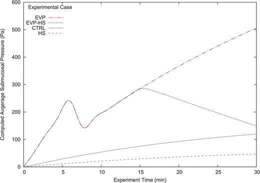
Average submucosal pressure (Pa) vs time (min) all computational experiments

It is evident from Fig. 5 that only the EVP and EVP-HS experiments reach the pressure threshold required to activate the damage model; this is commensurate with the experimental assumptions that the suturing procedure, coupled with a bolus injection of isotonic saline solution, induces acute edema. From Fig. 5 it is also observed that the HS computational case corrects for the slightly higher average pressure profile seen in the CTRL case as, possibly, a result of the surgically induced trauma leading to a slight drop in |$\varPi _V$|⁠. Moreover, the primary clinical hypothesis that administration of 7.5% HS solution may be an effective resuscitation fluid for reversing acute edema is observed; comparing the EVP curve to the EVP-HS curve a steady decline in the interstitial pressure can be seen, beginning at approximately at the 15-minute mark, coincident with HS injection. The interstitial pressure for the EVP-HS case nearly approximates that that of the CTRL case by the end of the computation; this is consistent with laboratory results.

Another closely related aspect of the computational model to clinical experiment is the average pressure in the individual layers of the intestine; in the experimental procedure, only the submucosal pressure values were measured. Fig. 6(a–d) shows the computational model predictions for each layer of the intestine over the duration of the clinical experiment. Consistent with the findings of a previous model (Young et al., 2012) we see that the average layer pressure is highest in the submucosa and musculature across all experiments. For the CTRL and HS cases, Fig. 6(a and b), the average pressures are nearly identical in every layer of the intestine. Conversely, at the conclusion of the experiment, the EVP case [Fig. 6(c)] displays an interlayer mucosal pressure difference of approximately 100 Pa, and for the EVP-HS case [Fig. 6(c)] approximately 10 Pa.

Fig. 6.

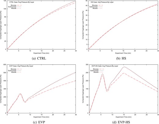
Average layer pressure (Pa) vs time (min) all computational experiments

However, the improved model predicts, contrary to the early model Young et al. (2012), that the absolute maximum pressure often occurs in the mucosa near the lumen where the capillary concentration is the highest; see Fig. 7 where the intestinal geometry has been sliced to allow for a comprehensive view of the pressure distribution throughout each layer. Moreover, it is clearly seen that the effects of the HS injection manifest most prominently in the mucosa for the EVP-HS case; c.f. Fig. 7(p–t).

The difference in the average versus maximal pressure distribution can be explained simply by the fact that the mucosa occupies a significantly larger area, and that the maximal pressures typically occur in a localized mucosal region near the lumen; in addition, for the EVP and EVP-HS cases, the mucosa undergoes large changes in volume. This difference was not observed with the simpler, explicit model (Young et al., 2012), which predicted minimal pressure profiles in the mucosal region and may be due to the lack of capability of the previous model to take into account the constrained storage coefficient of the tissue and its related effects.

Fig. 7.

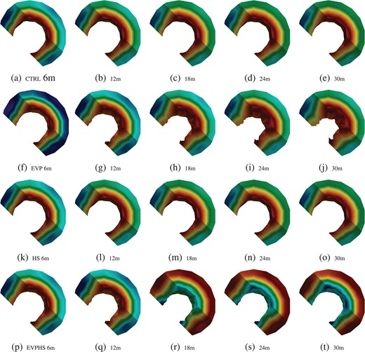
Intestinal hydrostatic pressure (Pa) distribution, all simulations; shading is with respect to the corresponding relative ranges in Table 9. Refer to the online version of the article for the colored figure; blue is the lowest relative value while warmer values are higher and red is the maximal relative value.

Fig. 8.

Lumen radius dilatation, all simulations

In addition to the relative distribution of pressures, the proposed improved model of intestinal edema formation allows for the comparison of lumenal radius dilatation across the various experimental regimes. Fig. 8 shows an overhead view of intestinal geometry; color has been suppressed to facilitate a direct comparison of the computational predictions for the radius of the lumen across the various experimental cases. It is immediately apparent that the EVP test case [Fig. 8(f–j)] yields a prediction of significant lumenal volume attenuation. This is consistent with the clinical observation that edema can significantly reduce the capacity for intra-lumenal transport of content through the intestine (Cox et al., 2008; Moore-Olufemi et al., 2005a,b; Radhakrishnan et al., 2006).

The computational model also predicts a slight decrease in the lumen radius for the CTRL case [Fig. 8(a–e)], which is consistent with the lower-than-normal oncotic blood pressure, |$\varPi _V$|⁠, found in the calibration process. The latter fact, as previously mentioned, is consistent with the clinical observation (Böck et al., 1989; Golab et al., 2011; Lucas et al., 1982; Öhqvist et al., 1980) that |$\varPi _V$| can decrease slightly as a result of the trauma associated with surgical preparation and procedure. Comparing the CTRL case [Fig. 8(a–e)] with the HS case [8(k–o)] it is observable that the slight decrease in lumen radius of the former case is abetted in the latter case; this points to the effectiveness of HS as a resuscitative medium in the context of routine surgical practice.

Finally, and most prominently, the effects of HS in restoring lumenal volume in the case of acute edema formation is clear when comparing the EVP case [Fig. 8(f–t)] to the EVP-HS case [Fig. 8(p–t)]. Not only does the administration of HS, occurring at the 15-min mark, reverse the initial lumenal attenuation induced by the initial bolus of isotonic saline (e.g. the initial EVP experimental setup) but also the final EVP-HS lumenal radius [Fig. 8(t)] is a close approximation to the final lumenal radius of the CTRL case [Fig. 8(e)]. This resuscitation effect was a primary hypothesis of the clinical study by Cox et al. (2008) motivating the model development and is clearly observed in the comparison of the respective sub-figures of Fig. 8.

Table 10

Final fluid volume relative to initial state. |$P_V=20$| mmHg for EVP and EVP-HS

Relative volume gain (%)
Experiment	6 min	12 min	18 min	24 min	30 min
CTRL	0.8	1.5	2.0	2.4	2.8
HS	0.3	0.6	0.8	1.0	1.1
EVP	5.5	9.9	13.4	16.0	18.0
EVP-HS	5.5	9.9	10.9	8.7	6.5

We close this section with a mention of relative volume gain predicted by the computational experiment. In the clinical case (Cox et al., 2008) a selection of the intestinal tissue was harvested post-experiment from the EVP and CTRL experimental cases; the tissue was weighed, subsequently allowed to dry and weighed once more. Comparing these values allowed for an assessment in the relative fluid volume gain for the EVP case (Young et al., 2012) with a mean value of |$19.8\%$|⁠. Computationally, the relative volume gain was estimated by comparing the initial volume of the mesh to the final, deformed volume; these results are reported in Table 10. The computed relative volume gain is predictive in the sense that the parameter calibration, mentioned for the CTRL and EVP cases, did not take into account relative volume gain for any parameter choices; only the average submucosal pressure, closely related to the clinically measured value, was utilized in the calibration process.

The computational model predicts an |$18\%$| relative volume gain for the EVP case (Table 10, EVP case) at mean |$P_V$|⁠; this is a relatively reasonable approximation to the clinical measurement of a mean volume gain of |$19.8\%$|⁠. Table 10 shows that the computational model also predicts less volume gain for the HS experiment versus the CTRL experiment, which is consistent with the lumenal radius observations seen in the corresponding sub-figures of Fig. 8. Moreover, Table 10 offers additional quantification of the resuscitation effects of the 7.5% HS injection (e.g. the EVP-HS case). Comparing the EVP, EVP-HS and CTRL cases of Table 10 the computational model predicts an approximate three-fold decrease in lumenal volume in the presence of acute edema formation (EVP vs. EVP-HS) and a two-fold increase in volume over the baseline control (EVP-HS vs. CTRL).

5.2 Estimating the impact of 7.5 HS resuscitation contractile capacity

In this section we posit an additional argument in support of the clinical hypothesis that 7.5% saline resuscitation could mitigate the early-onset effects of severe intestinal edema; specifically, we explore the impacts of resuscitation on improving motile function of the intestine through partially restoring contractile capacity. In the clinical study by Cox et al. (2008), this inference supporting improved contractile function following HS administration was made based on observations regarding reduced volume-induced internal stress on the muscle and mucosal layers. Here we discuss an alternative argument in support of this hypothesis using the computational model predictions for bulk volume gain to infer a possible impact on changes in an average diffusion distance, for ions signaling contraction, due to interstitial enlargement.

Note that the current model and the previous simplified model (Young et al., 2012) do not contain explicit terms accounting for ion diffusion directly; as noted in review, coupling an explicit ion diffusion model with the edema framework would further strengthen predictions. Nevertheless, the current model is capable of inferring that a distinct change in average ion diffusion length, in the acute-edema (EVP) versus resuscitated edema (EVP-HS) case, is strongly plausible. To establish this conclusion we combine computational results from Section 5.1 and a formula discussed in Section 5.2.1 to estimate, and infer, the possible effects. In our previous work (Young et al., 2012) a similar argument was made for an early model that does not incorporate the intrinsic storage coefficient of the tissue; however, the argument was made for only for the acute-edema (EVP) case and no derivation was offered. Here it is observed that the improved model, incorporating the intrinsic storage coefficient, yields a higher lower-estimate for the ion diffusion length in the case of acute edema; this shows that incorporating the parameter into the model may be of significance in clinical studies. In addition, in this manuscript, the technique is also employed to gauge the impact of HS resuscitation (EVP-HS).

Section 5.2.1 overviews the basic premises leading to (5.6). Section 5.2.2 employs (5.6) to approximate the change in interstitial distance between the acute-edema (EVP) and resuscitated edema (EVP-HS) case. Section 5.2.3 builds on the results of Section 5.2.2 and discusses the support for the altered contractility capacity hypothesis.

5.2.1 Intestinal motility in the presence of acute edema and resuscitation

The motility of lumenal content through the small bowel is enabled by contractions in the smooth muscle cells of the muscularis externa. Contractions are signaled by the diffusion of ions exiting a cell of Cajal or enteric neuron’s synapse, crossing the interstitial space, and received by channels proximal to the smooth muscle cells. Excess interstitial fluid enlarges the interstitial region between cells and increases the distance ions must traverse to reach their destination. Interstitial enlargement may cause a decrease in signaling capacity and reduce contractile activity, due to the increased diffusion length. Clinical experiment suggests administration of |$7.5\%$| HS may restore contractile function to ileus-stricken tissue via a reduction in the volume-induced stress (Cox et al., 2008). In this section we posit an additional argument in support of the primary clinical hypothesis; this argument is based on an approximation of the in vivo increase in average synaptic diffusion length using the results of the computational clinical experiments. In a previous work (Young et al., 2012) a similar argument was made for an early model that does not incorporate the intrinsic storage coefficient of the tissue; furthermore, the argument was made for only for the acute-edema (EVP) case and no derivation was offered. Here it is observed that the proposed model, incorporating the intrinsic storage coefficient, yields a higher lower estimate for the ion diffusion length in the case of acute edema; this shows that incorporating the parameter into the model may be of significance in clinical studies. In addition, the technique is also employed to gauge the impact of HS resuscitation, and a discussion of the diffusion length estimation methodology is put forth.

The porosity of the muscle layer of the intestine is approximated by way of a simplified representative elementary volume. Following this the increase in average distance between smooth muscle cells post-edema is inferred; this yields (5.6), which expresses the deformed distance in terms of the relative bulk volume gain of the intestinal muscle layer. In Section 5.2.2, (5.6) is applied to judge the relative difference between the control (CTRL), acute edema (EVP) and HS resuscitated acute edema (EVP-HS) computational test cases in order to estimate the impact of acute edema and HS resuscitation in vivo. The average size of a smooth muscle cell is between 2- and 4-|$\mu $|m wide, and 150-|$\mu $|m long (Lane, 1965), with an average distance between neighboring smooth muscle cells in the range of 2–30 nm (Alberts et al., 1994; Devine et al., 1971). Approximating a smooth muscle cell as a cylinder with average radius between 2- and 4-|$\mu $|m wide allows the construction of a simplified 2D, cross-sectional, representative elementary volume with length 1 cm and height equal to the radius of the cell plus the average gap size. The porosity, |$\phi $|⁠, in the representative elementary volume can then be estimated as |$\phi \approx 22\%-24\%$|⁠. Smooth muscle cells express a range of phenotypes and a porosity estimate of 22%–24% is consistent with smooth muscle tissues whose purpose is almost exclusively contractile in nature; such porosities are typically between 15% and 30% (Campbell & Campbell, 1995).

In the context of edema the interstitium, e.g. the white area between the cells in Fig. 9, fills with additional fluid and pushes the cells, shaded gray, apart. The value of |$r$|⁠, before and after edema, can now be approximated. Using this approximation, an estimation of the horizontal gap length, e.g. the horizontal distance between neighboring cells in the same row of Fig. 9, can then be made. The symbol |$\hat{r}$| is used to indicate the distance |$r$| post-edema. Letting |$r_c$| denote the cell radius and |$r_g$| be half the horizontal, or vertical, gap length we have |$r = \sqrt{2(r_c + r_g)^2}$|⁠. Following edema the change in base length, in Fig. 9, is given by |$\textrm{d}(r_c + r_g) = \textrm{d} r_c + \textrm{d} r_g$|⁠. Assuming that the smooth muscle cell is impermeable to interstitial fluid gives |$\textrm{d} r_c = 0$|⁠; thus the post-edema length, |$\hat{r}$|⁠, is given by

$$\begin{equation} \hat{r} = \sqrt{2(r_c + r_g + \textrm{d} r_g)^2}. \end{equation}$$

(5.1)

Fig. 9.

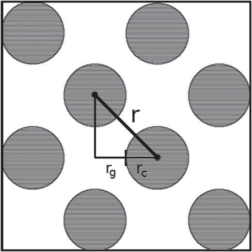
Smooth muscle distribution

Let |$V_s$|⁠, |$V_p$| and |$V_b$| denote the solid volume, pore volume and bulk volume, respectively, of the muscle layer tissue. Then |$V_b = V_s + V_p$| and |$\textrm{d}V_b = \textrm{d}V_s + \textrm{d}V_p$|⁠; dividing the previous expression through by an increment in pressure, |$\textrm{d}P$|⁠, and using the definition of compressibility (Bear & Bachmat, 1990; Merxhani, 2016) for the bulk (⁠|$C_b$|⁠), solid (⁠|$C_s$|⁠) and pore phases (⁠|$C_p$|⁠) gives

$$\begin{equation*} -V_bC_b = V_pC_p - V_sC_s. \end{equation*}$$

Assuming that the smooth muscle cell (solid phase) compressibility is much less than the tissue (bulk phase) compressibility gives |$-V_b C_b \approx V_p C_p$|⁠. This can be expressed as |$C_b \approx -\phi C_p$| where |$\phi = V_p/V_b$| is the porosity of the tissue. Substituting |$C_p = V_p^{-1} ({d}V_p / \textrm{d}P )$|⁠, |$C_b = -V_b^{-1}(\textrm{d}V_b / \textrm{d}P )$| and the definition of the porosity in |$C_b \approx -\phi C_p$| gives

$$\begin{equation*} \frac{\textrm{d}V_b}{\textrm{d}P} \approx \frac{\textrm{d}V_p}{\textrm{d}P}, \end{equation*}$$

from which the following relationship is obtained:

$$\begin{equation} \textrm{d}V_b \approx \textrm{d}V_p. \end{equation}$$

(5.2)

Now |$V_p = \phi V_b$| so that |$\textrm{d}V_p = \textrm{d}\phi V_b + \phi \textrm{d}V_b$|⁠; dividing through by |$V_p$|⁠, using the definition of the porosity |$\phi $|⁠, and (5.2) gives |$\textrm{d}\phi \approx \phi \left (1-\phi \right ) \textrm{d}V_p / V_p$|⁠. If we instead divide by |$V_b$|⁠, use the definition of |$\phi $|⁠, and (5.2) we have |$\textrm{d}\phi \approx \left (1-\phi \right )\textrm{d}V_b / V_b$|⁠. These results taken together yield

$$\begin{equation} \frac{\textrm{d}V_p}{V_p} \approx \frac{1}{\phi}\frac{\textrm{d}V_b}{V_b}. \end{equation}$$

(5.3)

Supposing that the interstitial area between cells can be approximated by |$V_p = Cr_g^2$|⁠, in 2D with |$C>0$|⁠, it follows that

$$\begin{equation} \frac{\textrm{d}V_p}{V_p} = \frac{2\textrm{d}r_g}{r_g}. \end{equation}$$

(5.4)

Substitution of (5.4) into (5.3) gives

$$\begin{equation} \textrm{d}r_g \approx \frac{r_g}{2\phi}\frac{\textrm{d}V_b}{V_b}. \end{equation}$$

(5.5)

Substitution of (5.5) into (5.1) yields an expression for |$\hat{r}$| in terms of the relative bulk volume change |$\textrm{d}V_b/V_b$| via

$$\begin{equation} \hat{r} \approx \sqrt{2\left(r_c + r_g \right)^2 + 2\left(r_c + r_g \right)r_g y_b + \frac12 r_g^2y_b^2} \end{equation}$$

(5.6)

where |$y_b = \phi ^{-1}\left (\textrm{d}V_b / V_b\right )$|⁠. The quantity |$\textrm{d}V_b/V_b$| has been measured for the computational model experiments, and the porosity estimate used is |$\phi \approx 23\%$|⁠.

5.2.2 Estimating the change in interstitial distance

In order to establish a baseline for the estimation of the in vivo effects of edema on intestinal motility, (5.6) is applied to the results of the control computational test (CTRL). This baseline is then used to deduce the relative increase for both the acute edema (EVP) and resuscitated edema (EVP-HS) case. Conclusions are inferred regarding the invivo intestinal motility from this relative change. Let |$\hat{r}_c$| and |$\hat{r}_g$| denote the post-experimental cell radius and gap size, respectively, so that |$\hat{r} = \sqrt{2\left (\hat{r}_c + \hat{r}_g\right )}$|⁠. Using the cell fluid-impermeability assumption (⁠|$\hat{r}_c = r_c$|⁠) average ranges for |$\hat{r}_g$| can be estimated for each computational case; results are shown in the table of Fig. 10. According to Fig. 10 the values of |$\hat{r}_g$| for the case of acute edema (EVP) are between |$7.71$| and |$8.09$| times larger with respect to the control case. For the HS resuscitation (EVP-HS) case the average value of |$\hat{r}_g$| is between |$2.36$| and |$2.43$| times higher than those of the control.

Fig. 10.

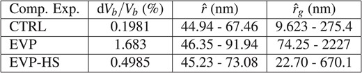
Computed relative bulk volume gain and gap size estimation

5.2.3 Impact on intestinal motility

In Section 4.4.1 it was discussed that a slightly lower oncotic blood pressure was found to produce computational results consistent with those of the clinical experiment and that this could be due to trauma incurred by the surgical preparation procedure, etc. An increase in the interstitial distance between smooth muscle cells may be a primary factor in impaired contractility and intestinal motility due to the increased length that ions must diffuse. The purpose of this section is to compare approximations of the invivo interstitial distance for the EVP and EVP-HS cases, modulated primarily by |$\hat{r}_g$|⁠. We conclude, based on the estimations, that HS resuscitation could show promise for restoring intestinal motility.

To compare approximations for the EVP and EVP-HS interstitial distances, Fig. 10 is used to determine the relative values |$\gamma _{EVP} = (\hat{r}_g^{EVP}/\hat{r}_g^{CTRL})$| and |$\gamma _{EVP-HS} = (\hat{r}_g^{EVP-HS}/\hat{r}_g^{CTRL})$|⁠. It is assumed that under normal in vivo conditions the interstitial distances, for EVP and EVP-HS, can also approximated by these proportions. From Fig. 10 we see that |$\gamma _{EVP}$| takes on values between 7.716 and 8.09, likewise |$\gamma _{EVP-HS}$| lies between 2.359 and 2.433. As discussed in 5.2 the average in vivo distance between smooth muscle cells for healthy, non-surgically treated specimens is between approximately 2 and 30 nm (Devine et al., 1971; Alberts et al., 1994).

Based on the assumption of relative proportions being preserved, the values for |$\gamma _{EVP}$| infer an average interstitial distance between 15.432 and 242.7 nm in the case of acute edema. Likewise, the values of |$\gamma _{EVP-HS}$| infer average interstitial distances between 4.718 and 72.99 nm for acute edema resuscitated by |$7.5\%$| HS. The theoretical optimal length for the transmission of ion signals is postulated to lie within the range of 12–20 nm, with transmission distances beyond this distance being associated with reduced signaling capacity (Savtchenko & Rusakov, 2007). Thus, the administration of HS in vivo should lower the average interstitial distances between cells by a factor of approximately 3.3. Thus, it is reasonable to expect that resuscitation of acute edema with |$7.5\%$| HS solution could realize a significant restoration of contractile function, and result in at least partially restoring intestinal motility. This result provides a new avenue of reasoning in agreement with the conclusion of the clinical hypothesis (Cox et al., 2008), e.g. that of reduced motility in the case of acute edema and the action of HS in restoring contractile function.

5.3 Model clarifications and further experimental suggestions

The proposed model of intestinal edema formation described in this manuscript combines the Starling–Landis–Drake–Laine clinical model of microvascular filtration and lymphatic exchange, with the equations of poroelasticity, thus coupling the clinical models of fluid exchange with the mechanical response of the intestinal tissue. In addition, the model incorporates a compensation for the overestimation of the Starling equation for high values of |$P_V$| and incorporates a model of local tissue damage to the layered structure of the intestine. Due to the complexities of the model, there are several aspects that could be improved with additional experimental evidence.

First and foremost, additional clinical insight into constituents of the model would be highly beneficial. For instance, differences in the computational submucosal pressure averages versus reported submucosal transducer measurements may be further improved with additional parameter information. Some of this information, such as bulk |$\varPi _V$| before and after saline injection, may currently be measurable experimentally for the pre-and-post edema cases. Additional information on the combined permeability, |$\kappa $|⁠, of the intestine and the constrained storage coefficients, |$c_1$|⁠, of the individual intestinal layers would also be welcome. These quantities have been measured in various ways for other tissue beds (Durand et al., 1981). Measurements of the constrained storage coefficients, |$c_1$|⁠, may possibly be approximated by the use of exvivo clinical approaches such as the growth of appropriate tissue matrices on scaffolds Beatty et al. (2002) for use in subsequent measurements of mechanical properties. Enhancements to the damage model, including the localization of |$\mu $| and |$\lambda $| parameter changes based on soft-tissue injury studies, could provide further insight.

Another aspect of the model that could be clarified by additional clinical experiment is the effect of high venous pressure on microvascular fluid flows; such effects include Starling overestimation and the impacts of high venous pressure on the various parameters in the Starling model. A clarified statistical understanding of the relationship of the |$(K_f,\sigma )$| variation for venous pressures exceeding |$15$| mmHg (⁠|$2000$| Pa) seems to be lacking in the clinical literature. Moreover, a quantified understanding of the |$(K_f,\sigma )$| relationship to both |$P_V$| and the lymphatic pumping pressure, |$P_p$|⁠, could improve the fluid model at high venous pressures.

It is known that a number of physiological ‘safety factors’ exist to ward against the formation of edema (Kviets, 2010), but begin to break down near venous pressures exceeding |$P_V \geqslant 15$| mmHg. A further complication in this regime is that experimental evidence suggests (Adamson et al., 2004; Hu et al., 2000; Levick, 2004) flow may be driven more by local, rather than bulk, values of the oncotic pressures, |$\varPi _V$| and |$\varPi _I$|⁠, and that the Starling equation, used with bulk tissue oncotic pressure values, may overestimate the microvascular fluid exchange as these values fluctuate locally. It is not presently clear if this dynamic implies that local micro-scale models, such as Adamson et al. (2004) and Hu et al. (2000), of the vascular endothelium are strictly necessary or if a homogenized correctional factor, endeavored here, can be reliably deduced from statistical approaches applied to experimental data that is robust with respect to a wide range of venous blood pressures.

Fig. 11.

Admissible experimental |$P_V$| (deca Pa) vs. computed average submucosal pressure (Pa) EVP experiment; |$P_V\in [17,23]$| mmHg, |$[227,307]$| dPa

In the current model, the basic approach of calibration of the |$(K_f,\sigma )$| pair, and its coupling to |$P_p$|⁠, was done by selecting |$K_f$| and |$P_p$| from an early model (Young et al., 2012) and employing the EVP experiment to find a suitable reduction in |$\sigma $| at the mean venous pressure of |$20$| mmHg (⁠|$2666$| Pa) observed in the clinical trials. The choices of |$K_f$| and |$P_p$| (see Table 7) coincide with the known clinical heuristic observation (Maron et al., 2001; Scallen et al., 2010) that as |$P_V$| raises, |$K_f$| and |$P_p$| also increase, and that an increase in |$K_f$| implies a decrease in |$\sigma $|⁠. In the clinical literature, however, the specifics of this relationship seem largely unexplored and the current understanding is limited to this qualitative description.

A variation of |$P_V$| parameter test for the EVP computational case was conducted to test the voracity of the single-calibration approach for |$(K_f,\sigma )$| and |$P_p$| at median |$P_V$|⁠. In the clinical experiment (Cox et al., 2008), measured values of |$P_V$| were reported to lie in the range of |$[17,23]$| mmHg (i.e. [2266,3066] Pa). The computational model was run using the fixed values of |$K_f$| and |$P_p$|⁠, and calibrated |$\sigma $|⁠, assessed for the |$P_V=20$| mmHg (⁠|$2666$| Pa) case, as mentioned above. The computational results are shown in Fig. 11 with |$P_V=20$| mmHg (2666 Pa) corresponding to the middle bar and average computational submucosal pressures (in Pa) reported on the |$y$|axis.

The sample standard deviation of the average submucosal pressures, over all computational experiments, is |$0.84$| mmHg (⁠|$112$| Pa), which higher than the experimentally reported value of |$0.34$| mmHg (⁠|$45$| Pa). However, if we consider the computational standard deviation for the experiments in a ‘nearby neighborhood’ of the mean value |$P_V=20$| mmHg (2666 Pa), used for calibration, such as |$P_V \in [19,21]$| mmHg (or |$[2533,2800]$| Pa) then the standard deviation more closely matches the experimental standard deviation of |$0.34$| mmHg (⁠|$45$| Pa) at a value |$0.39$| mmHg (⁠|$52$| Pa). This indicates that using a single calibration around the mean vascular pressure may not be sufficient in accurately capturing the full dynamics of the |$(K_f,\sigma )$| and |$P_p$| relation across the large variation in |$P_V$|⁠. We infer, then, that clinical experiments exploring this relation will be useful in constructing a more accurate computational model.

Despite the benefit that additional clinical understanding could offer the model, the predictive HS and EVP-HS computational experiments resulted in average submucosal pressures within the experimentally observed range. Based on the model observations, discussed in Sections 4.4, 5.1 and 5.2 we agree with the clinical suggestion (Cox et al., 2008) that the HS resuscitation technique offers promise in controlling the formation of acute edema in the presence of high venous pressure.

Nevertheless, the proposed computational model could be quite useful to clinicians. The computational average submucosal pressures for all cases are within experimental ranges, the final fluid content (EVP) is closely predicted, and the qualitative properties of the impact of HS administration in abetting acute edema are clearly observed. For these reasons, the proposed model may provide an effective qualitative benchmark for clinical research into the formation of edema in the intestine and for the a priori judgment of the relative impact of various resuscitation fluids, in abetting edema, during a short-time (e.g. 5–60 min) window. Moreover, as further clinical understanding around the relationship between |$K_f$|⁠, |$\sigma $| and |$P_p$|⁠, in the |$P_V \geqslant 15$| mmHg regime, become well understood or as values for material parameters, such as |$c_1$| and |$\kappa $|⁠, within the intestine become available the model can be easily improved.

6. Conclusion

In this paper, we have described a numerical model of edema formation, based on the solution of Biot’s equations and have demonstrated the potential suitability of the model in medical applications via the context of a clinical experiment in intestinal edema formation (Cox et al., 2008). Physical parameters used in Biot’s model were selected from the clinical literature for specific use in the intestine, or estimated using values from related organs where intestine-specific values were unavailable. The numerical approach, suitable for intestinal modeling, is a novel extension of a previous discretization proposed by the authors (Rivière et al., 2017); the model is implicit and has previously been shown to abet spurious oscillations in the pressure when used with dual penalty parameters (Rivière et al., 2017). These features confer some advantages over explicit approaches (Young et al., 2012) such as a less restrictive time-step requirement and the ability to model physically non-zero storage coefficients in the mass conservation equation (3.4).

In addition to the numerical and modeling advantages we have included a damage model for the tissue to account for the effects of excessive fluid pressures encountered in severe edema in addition to a capillary density in the fluid model approximating a physiological microvascular distribution (Granger & Barrowman, 1984; Young et al., 2012). In addition, computational results suggest that the inclusion of the specific storage coefficient, unavailable in early models of intestinal edema (Young et al., 2012), may be strongly advantageous for clinically related results.

Motivated by clinical experimental results (Hu et al., 2000) we proposed a simple extension of the fluid balance model (4.1) to account for the over-estimation of Starling forces in the presence of high venous blood pressure, and local oncotic pressure gradients, that may arise in the case of fluid resuscitation via |$7.5\%$| HS. The over-estimation of Starling forces is an ongoing area of research in the clinical literature (Hu et al., 2000; Adamson et al., 2004; Levick, 2004). We have demonstrated that a calibrated, simplified model may be useful, from a computational standpoint, in edema models where more complex features of the microscale physiological features of vessel structures, such as the local characteristics of the endothelial glycocalyx, are not otherwise available.

Finally, the clinically observable model predictions (Fig. 6, submucosal plot) of the clinical voracity of HS resuscitation for intestinal edema are in line with clinically observed results Cox et al. (2008). The proposed model is easily extensible as clinical experiments clarify additional relationships in the regime of high blood pressures, or as measurements of intestinal material properties are made available. Thus, the proposed method may show promise for clinicians modeling the effects of acute edema or fluid resuscitation agents in the planning of clinical experiments, or for various treatments.

Acknowledgements

The authors would like to acknowledge Drs Marie Rognes, Alexandra Diem and Cécile Daversin-Catty for the benefit of physiology-related discussions and clinical literature suggestions. Moreover, the authors also acknowledge the contributions of the late Dr Jennifer Young, whose work in pioneering early computational research models of intestinal edema formation continues as an inspiration to the community.

Funding

This research was conducted, in part, via the support of National Science Foundation (NSF-DMS 1312391). T. T. also acknowledges support from the Research Council of Norway under the FRINATEK Young Research Talents Programme project #250731/F20 (Waterscape).